Light Quark Mass Effects in Bottom Quark Mass Determinations

arXiv:hep-ph/0102292v2 26 Feb 2001

CERN-TH/2001-48 MPI-PhT/2001-01 February 2001 hep-ph/0102292

Light Quark Mass Effects in

Bottom Quark Mass Determinations

Andr´ e Hoang

Theory Division, CERN, CH-1211 Geneva 23, Switzerland

Recent results for charm quark mass effects in perturbative bottom quark mass determinations from Υ mesons are reviewed. The connection be- tween the behavior of light quark mass corrections and the infrared sensi- tivity of some bottom quark mass definitions is examined in some detail.

Presented at the

5th International Symposium on Radiative Corrections (RADCOR–2000)

Carmel CA, USA, 11–15 September, 2000

∗

Permanent address: Max-Planck-Institut f¨ ur Physik, Werner-Heisenberg-Institut, F¨ohringer

Ring 6, D-80805 M¨ unchen, Germany.

1 Introduction

The mass of the bottom quark is an important parameter in the theoretical de- scription of B meson decays. In particular, for the extraction of V

and V

from inclusive decays a precision in the bottom quark mass of the order 1% is desirable due to a strong mass dependence. Precise determinations of the bottom mass are available from Lattice QCD using the B mesons mass (see Refs. [1] for recent re- views) and from perturbative QCD. As the B meson binding energy is dominated by non-perturbative QCD, perturbative methods can only be applied to Υ mesons, where the relevant dynamical scales, momentum h p i ∼ M

v and energy h E i ∼ M

v

, v being the bottom quark velocity, can be larger than the hadronization scale Λ

.

In recent time new perturbative bottom mass analyses have been carried out in- cluding newly available NNLO (i.e. O (v

, α

v, α

)) corrections in the non-relativistic expansion for heavy quark–antiquark systems based on the concept of effective theo- ries and employing properly defined short-distance quark mass definitions

that are adapted to the non-relativistic framework [3]. It has become practice to determine the bottom MS mass m

(m

) as the reference mass to compare the various analy- ses among each other. The various results, which are based on experimental data on the Υ mesons, show good agreement with a central value for m

(m

) of about 4.2 GeV and an uncertainty ranging from 50 to 80 MeV. It is important to note that the uncertainty is predominantly theoretical, and (as a necessary consequence) partly depends on the taste and believes of the respective authors. It is therefore impossible to interpret the value for the error in a statistical way. It will be the primary aim of future studies and analyses to achieve a better understanding of this theoretical uncertainty—not necessarily in order to reduce it further, but in order to put it on firmer ground.

One effect that has been neglected in previous bottom quark mass analyses is com- ing from the finite masses of the light quarks (u, d, s, c), where ”light” means ”lighter than the bottom quark mass”. In this talk I report on results and examinations on light quark mass corrections at NNLO in the non-relativistic expansion which have been presented in Refs. [4,5]. Light quark mass corrections are interesting because the non-relativistic bb system is governed by a tower of scales: M

, h p i ∼ M

v and h E i ∼ M

v

. For small velocities these scales form a hierarchy and their relations to Λ

determines the theoretical approach that has to be used to describe the bb dynamics. In the work discussed in this talk I assume that all three scales are much larger than Λ

(i.e. that v is not smaller than about 0.3 for bottom quarks) as only for this case the relevant approach is well understood theoretically.

Whether the mass of a light quark can also be considered ”light” in the context of the non-relativistic bb dynamics depends on its relation to the three scales mentioned

1

At LEP the MS bottom mass at the Z scale has been determined from the rate of 3 jet events containing a bb pair [2]. This measurement established experimentally the ”running” of the bottom MS mass. For this method, the uncertainties are, however, still too large that light quark mass effects would be irrelevant.

2

I call a heavy quark mass definition without an O (Λ

) ambiguity a short-distance mass.

above. The masses of the up, down and strange quarks are indeed much smaller than any of the three scales and one can expect that for them the massless approximation is a very good one, as an expansion in their masses is justified. The mass of the charm, however, can be about as large as h p i and larger than h E i , and it is clearly inappropriate to consider the massless approximation in the first place. I will show that the effects of the non-zero charm quark mass in bottom mass determinations can amount to up to several tens of MeV depending of the method and the bottom short-distance mass definition that is employed.

Apart from the resulting quantitative effects in the determination of bottom quark short-distance masses, light quark mass effects are also interesting conceptually be- cause the massive quark loops provide an infrared cutoff of the momentum flow through gluon lines. The behavior of light quark mass corrections, in general, can therefore serve as a natural tool to monitor the degree of infrared (IR) sensitivity of various bottom quark mass definition and their resulting ambiguity. This is in close analogy to the well-known IR renormalon studies with a fictitious gluon mass, but with the difference that the light quark mass corrections are real.

2 Light Quark Mass Corrections in the Coulomb Potential

In order to account for the light quark mass effects in the non-relativistic quark- antiquark dynamics at NNLO we have to determine the light quark mass corrections to the Coulomb potential V

( r ) = −

+. . . that occurs in the Schr¨odinger equation

− ∇

M

− ∇

4 M

+

V

( r ) + . . .

− E

G( r , r

, E) = δ

( r − r

) . (1) Here M

is (just as a matter of convenience in writing down Eq. (1)) the bottom pole mass and E = E

− 2M

, E

being the center-of-mass energy. At NNLO, corrections to the Coulomb potential have to be taken into account up to order α

. For massless light quarks these two-loop corrections have been determined in Refs. [6]. At NNLO there is also a potential of order α

/(M

r

) and another of order α

/(M

r). (The latter contains e.g. the Darwin and the spin-orbit interactions.) For these potentials light quark mass corrections do not have to be considered because they contribute only at NNLO, whereas for light quark mass corrections we gain at least one more power of α

. There are also no light quark mass corrections to the kinetic energy terms.

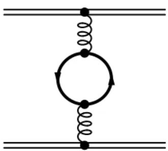
The light quark mass corrections to the Coulomb potential arise for the first time at order α

from the insertion of the light quark self energy into the gluon line (Fig. 1).

These corrections contribute at NLO in the non-relativistic power counting. For one massive light quark flavor, and the other n

− 1 light quark flavors being massless, the correction reads ( ˜ m

= e

m

):

δV

( r ) = − C

α

r

α

3 π

ln( ˜ m

r) + 5 6 +

∞

Z

1

dxf (x) e

,

Figure 1: NLO contribution to the static potential coming from the insertion of a one-loop vacuum polarization of a light quark with finite mass.

f (x) ≡ 1 x

√ x

− 1 1 + 1 2 x

. (2)

The light quark mass corrections vanish for m

r → 0. This is related to the definition of α

that is (here and for the rest of this presentation) chosen to include the evolution originating from the massive light quark. In other words, the massive light quark is not integrated out. I emphasize that the statements about the size and behavior of the light quark mass corrections I will make later, are only true for this definition of α

. It is straightforward to generalize Eq. (2) to arbitrary numbers of massive light quark species and different definitions of α

. However, I emphasize that all previous analyses, where the light quark masses were neglected have naturally adopted the same scheme, so the results discussed here can be directly interpreted as additive corrections.

In Eq. (2) the NLO light quark mass corrections to the Coulomb potential are given in terms of a subtracted dispersion relation, where f is the absorptive part of the vacuum polarization. This representation is advantageous for determining the effects of the light quark masses to heavy-quark–antiquark bound state properties in Rayleigh-Schr¨odinger perturbation theory due to the simplicity of the dependence on r . The remaining dispersion integration can then be carried out numerically (or if possible analytically) at the very end. In particular, for the determination of multiple potential insertions at higher orders in time-independent perturbation theory this method is probably the only feasible one. On the other hand, the dispersion representation makes the choice of definition for α

manifest.

At NNLO the light quark mass corrections to the Coulomb potential arise from dressing the one-loop diagram in Fig. (1) with additional gluon, ghost and light quark lines. The resulting diagrams where calculated numerically by Melles [7]. Using again the dispersion relation representation it is possible to rewrite Melles’ results in a form that is simple to use for determining the light quark mass corrections. With the same conventions as for the NLO result, and adopting the pole mass definition for m

, the result reads [5]:

δV

( r ) = − C

α

r

α

3 π

3

ln( ˜ m

r) + 5

6 β

ln(˜ µ r) + a

2

+ β

π

4

− 3 2

∞

Z

1

dx f(x) e

β

ln m

µ

+ g

(x, m

, r) − a

−

−

ln( ˜ m r) + 5 6

− π

12 +

∞

Z

1

dx f (x) e

g

(x) + g

(x, m

, r) − 5 3 +

57 4

ln( ˜ m

r) + 161 228 + 13

19 ζ

+ c

∞

Z

c2

dx

x e

+ d

∞

Z

d2

dx

x e

, (3) where

g

(x, m

, r) = ln(4x

) − Ei(2 m

x r) − Ei( − 2 m

x r) , g

(x) = 5

3 + 1 x

1 + 1 2 x

√ x

− 1 (1 + 2x

) ln x − √ x

− 1 x + √

x

− 1

. (4) The first three lines in Eq. (3) are exact and involve corrections coming from one and two insertions of the one-loop massive light quark vacuum polarization. The fourth line involves all other corrections and is parametrized by four numerical constants.

Of these constants only two are independent, because the corrections have to vanish for m

→ 0. A useful parameterization of the constants reads [5]

c

= ln

2

ln

2

, d

= ln

ln

2

, A = exp

161 228 + 13

19 ζ

− ln 2

, (5)

where for the constants c

and d

one can obtain the following numerical results from the results of Refs. [7],

c

= 0.470 ± 0.005 d

= 1.120 ± 0.010 . (6)

3 1S Mass, n = 1 ³ S 1 Binding Energy and Upsilon Expansion

Naively one might think, that – at least up to some non-perturbative effects – the mass spectrum for bb mesons could be obtained from solving the Schr¨odinger equation (1). However, the theoretical formalism from which it has been derived is becoming unreliable for higher radial excitations (n > ∼ 2), because the average momentum h p i ∼

and the average energy h E i ∼

become comparable or even smaller than Λ

.

For the ground state (n = 1), however, the formalism for the perturbative contri- butions is likely to work, and one can determine e.g. the MS value of the bottom quark mass from comparing the Υ(1S) mass with the result for the n = 1,

S

bb bound state energy once an estimate for the non-perturbative corrections is made [8,9].

On the other hand, one can use the perturbation series for a n = 1,

S

bound

state mass obtained from Eq. (1) as a formal short-distance mass definition, because

it is free of the strong linear infrared sensitivity that leads to an ambiguity of order Λ

in the the pole mass definition [10,11]. In Ref. [12] the so called 1S mass has been defined as one half of the perturbative n = 1,

S

bound state mass obtained from Eq. (1). It has been demonstrated that the 1S bottom quark mass leads to a very well convergent perturbative series for totally inclusive B decay rates [13]. Physically this behavior can be understood from the fact that the 1S mass is adapted to the situation where heavy quarks are very close to their mass shell, a situation that is realized for heavy-heavy as well as for heavy-light bound state systems. Heavy quark mass definitions that have this property are called ”threshold masses” [14]. There are other heavy quark threshold mass definitions in the literature, such as the PS mass [11] and the kinetic mass [15], which will, however, not be further discussed in this talk.

The light quark mass corrections to the Coulomb potential presented in the previ- ous section can be used to determine the light quark mass corrections in the bb bound state energies. Here we will, as indicated earlier, only consider the binding energy of the n = 1,

S

triplet ground state, but the calculation can be generalized without difficulty to arbitrary quantum numbers. In Dirac notation the NNLO result for the light quark mass corrections reads

2 ^h M

− M

i

m

= ^h M

− 2M

i

m

= h 1S | δV

| 1S i + h 1S | δV

| 1S i + ^X

i6=1S

Z

h 1S | δV

| i i h i | E

− E

δV

| 1S i

+ 2 ^X

i6=1S

Z

h 1S | δV

| i i h i | E

− E

V

| 1S i . (7) The first term on the RHS of Eq. (7) is the NLO correction of order M

α

(in the non-relativistic power counting) and the terms in the second and third line are the NNLO corrections of order M

α

. The explicit result based on the dispersion relation representation is given in Ref [5]. The NLO contribution has already been calculated earlier in Ref. [16] and agrees with the result here. The corrections coming from gluons and massless quarks (not displayed in Eq. (7), and called ”massless corrections” from now on) have first been calculated in Ref. [8].

It is not possible to use Eq. (7) directly for any phenomenological analysis that intends a precision better than order Λ

, because it is written in terms of the bottom pole mass. Nevertheless, it is instructive to have a closer look at the behavior of the ligh quark mass corrections in the bottom 1S-pole mass relation displayed in Eq. (7). For M

= 4.9 GeV, m

(m

) = 1.5 GeV for the MS charm quark mass and α

(µ = 4.7 GeV) = 0.216 we obtain

M

= ⁿ 4.9 − ^h 0.051 ⁱ

LO

− ^h 0.074 + 0.0045

i

NLO

− ^h 0.099 + 0.0121

i

NNLO

o GeV , (8)

where the charm mass corrections are indicated by the subscript m and the numbers without subscript are from the massless corrections. We stress that because M

α

≈ 1.5 GeV the charm mass correction shown in Eq. (8) cannot be obtained by an expansion in the light quark mass. To obtain the numbers shown in Eq. (8) it is essential that the complete expressions for the corrections given in Eqs. (2) and (3) are taken into account. We see that neither the massless corrections nor the charm mass corrections are converging. This is a consequence of the fact that I have used the bottom pole mass as an input parameter and the practical reason why Eq. (7) has only limited use for a phenomenological analysis. Another interesting point I would like to mention is that the NNLO charm mass corrections arising from double insertions of NLO potentials (the last two terms on the RHS of Eq. (7)) make for less than 10% of the full NNLO charm mass corrections for µ between 1.5 and 5 GeV.

This property will be important for the analysis of the charm mass effects in the Υ sum rules (Sec. 7).

It is interesting that the linear sensitivity to small momenta contained in the pole mass definition is directly reflected in the analytic behavior of the light quark mass corrections in Eq. (7) for m

→ 0 (a

≡ α

(µ)):

h M

− M

i

m

−→ − C

a

π

π

8 m

+ . . .

NLO

− C

a

π

π

16 m

β

ln µ

m

− 4 ln 2 + 14 3

− 4 3

59

15 + 2 ln 2

+ 76 3π

c

c

+ d

d

+ . . .

NNLO

. (9) Using the fact that the dispersion integrations in Eqs. (2) and (3) can be interpreted as an integration over a gluon mass, one can show (see Ref. [17]) that the linear light quark mass terms in Eq. (9) are directly related to the linear gluon mass terms frequently used in renormalon analyses. A different way to look at this feature is that the mass of the light quark provides an infrared cutoff for gluon lines due to decoupling at very small momentum transfers. On the other hand, if we express the 1S mass in terms of another short-distance mass, such as the MS mass, these linear light quark mass terms do not arise. I will come back to this point later in this talk.

I also would like to point out that the structure of the linear light quark mass

corrections in Eq. (9) themselves reveals their infrared origin. First of all, the linear

dependence on the light quark mass is non-analytic since it comes from the square root

of m

. On the other hand, the full vacuum polarization of the quark loop does only

depend on the square of the quark mass, so the linear mass terms cannot be obtained

from expanding in the light quark mass before doing the integration over the gluon

momentum. Consequently the linear mass terms arise from gluon momenta of the

order of the light quark mass. This feature is also reflected in the BLM scale in the

NNLO term in Eq. (9) which is of order m

rather than M

α

. Another observation is

that the non-analyticity of the linear mass terms is associated with an enhancement

factor π

. This is a common feature of contributions that originate from infrared momenta. We will see later that this enhancement will help us a lot to determine the three-loop light quark corrections to the MS-pole mass relation.

Another feature of expression (9) is that the linear light quark mass corrections at NLO (NNLO) are multiplied by α

(α

), which appears to contradict the non- relativistic power counting mentioned before. However, one has to take into account that the light quark mass corrections are M

times a function of the ratio m

/(M

α

).

Thus there is no contradiction with the non-relativistic power counting.

On the other hand, one can also show that the linear light quark mass terms are in fact completely independent of the quantum number of the bound state. This can be seen from the fact that the terms displayed in Eq. (9) are equal to the linear light quark mass terms contained in

[δV

( r ) + δV

( r )]. Because the linear terms are r- independent they are just multiplied by the norm of the bound state wave function, i.e.

by 1. [The suppression of the NNLO charm mass corrections from double insertions of NLO potentials mentioned above, can be understood from the dominance of the linear and r-independent light quark mass terms in the potential: constant corrections to potentials give zero in higher order time-independent perturbation theory.] This means that the term ∝ α

(α

) in Eq. (9), can equally well be considered as two (three) loop contributions. This interesting feature is giving us a direct hint how one has to combine a usual loop expansion in powers of α

(such as the perturbative series for the MS-pole mass relation) with a non-relativistic expansion that is in α

and the velocity v (such as the 1S-pole mass relation). The guiding principle to combine the two types of expansions is the cancellation of corrections that are linearly sensitive to small momenta. The resulting prescription is called upsilon expansion [13] and has been devised first for the massless corrections based on more general arguments.

The upsilon expansion states that we have to consider corrections of N

LO in the non-relativistic expansion (which contains itself a resummation of certain corrections to all orders in α

) as of order α

in the usual expansion in the number of loops.

4 Heavy Quark MS–Pole Mass Relation

The pole mass parameter is quite convenient in intermediate steps of calculating the dynamics of a non-relativistic QQ pair, because the Schr¨odinger equation takes its standard QED-like form only in the pole mass scheme (see Eq. (1)). However, for practical applications (were a precision better than Λ

is relevant) the pole mass needs to be replaced by a short-distance mass parameter. The standard choice is the MS mass definition.

The upsilon expansion tells us that, if we want to describe the non-relativistic QQ dynamics at NNLO, the heavy quark MS-pole mass relation has to be known at order α

. The massless two-loop corrections have been determined a long time ago in Ref. [18] and the massless three-loop corrections can be found in Refs. [19]. In Ref. [18]

3

At NNLO the energy scale M

α

does not yet arise as a relevant dynamical scale.

also the two-loop light quark mass corrections were determined fully analytically for any value of the mass. For m

≪ M

the light quark mass corrections at two loops read

h M

(M

) − M

i

m

−→ − C

a

π

π

8 m

− 3 4

m

M

+ . . .

. (10) It is remarkable that the linear two-loop term is equal to the NLO term displayed in Eq. (9). This is, of course, not an accident, but related to the universality of the linear light quark mass correction, already mentioned before. However, the reason for this is more general: it has been shown in Refs. [10,11] that the total static energy of a QQ pair, E

= 2M

+ V ( r ) is free of any linear dependence on small momenta to all orders of perturbation theory. Therefore, also the three-loop linear light quark mass corrections in [M

(M

) − M

] are given by the NNLO linear terms displayed in Eq. (9). From this fact alone we would not gain much because we cannot get any information on the size of the three-loop correction with higher powers of the light quark mass from this argument. However, we have seen before that the non- analytic linear light quark mass terms are enhanced by a factor π

with respect to the analytic terms with higher powers of the light quark mass. This feature is also clearly visible in Eq. (10). Comparing the size of the full two-loop light quark mass corrections to the size of the linear term we find that the difference is at most 15% for m/M

< 0.3. We therefore conclude (or conjecture) that the three-loop linear light quark mass corrections dominate the yet uncalculated full three-loop light quark mass corrections in a similar way and that the linear light quark mass terms provide a very good approximation at the level of 10% to the full light quark mass corrections. Some more numerical examinations based on BLM type three loop corrections have been carried out in Ref. [5] and are compatible with the conjecture. It even seems likely that the two- and three-loop differences between linear mass approximation and full results have a different sign, so that the difference in the sum might be much below 10%.

To conclude the discussion of the light quark mass corrections to the MS–pole mass relation let me also show some numerical values. For M

(M

) = 4.2 GeV, m

(m

) = 1.5 GeV for the MS charm quark mass and α

(µ = 4.7 GeV) = 0.216 we obtain

M

= ⁿ 4.2 + ^h 0.385 ⁱ

+ ^h 0.197 + 0.0117

i

+ ^h 0.142 + 0.0176

i

o

GeV . (11)

The massless corrections are somewhat better behaved than for the 1S-pole mass relation (but not what one would honestly call ”convergent”), but the charm mass corrections (which are in the linear approximation) are again quite badly behaved.

If we evaluate the charm mass corrections for µ = m

(m

) = 1.5 GeV, which is the

natural scale for the linear mass terms, we obtain 36 MeV for the order α

corrections

and 32 MeV for the order α

terms.

5 Heavy Quark MS–1S Mass Relation

The perturbative relation between the bottom 1S and the MS mass can be used for two purposes. First, one can extract the bottom MS mass from the experimental number for the mass of the Υ(1S) (with a model-dependence from the estimate of non-perturbative corrections). Second, one can determine the bottom MS mass from determinations of the 1S mass from methods that are less sensitive to non-perturbative effects, such as the Υ sum rules.

Using the results of the two previous sections and combining them using the upsilon expansion to eliminate the pole mass parameter (which is absolutely crucial!) it is straightforward to derive this relation to order α

(or NNLO in the non-relativistic expansion). The full analytic expression for the resulting perturbative series can be found in Ref. [5].

To illustrate the behavior of the series let me show here again some numerical results. For M

= 4.7 GeV, m

(m

) = 1.5 GeV and α

(µ = 4.7 GeV) = 0.216 we obtain

M

(M

) = ⁿ 4.7 − ^h 0.382 ⁱ

− ^h 0.098 + 0.0072

i

− ^h 0.030 + 0.0049

i

o

GeV . (12)

Comparing this result to Eqs. (8) and (11) we see that now the massless corrections show a quite good convergence and the charm mass corrections a fairly good one.

This behavior reflects the fact that the MS and the 1S mass definition both are short- distance masses, i.e. they do not have an ambiguity of order Λ

such as the pole mass. It is therefore possible to reliably extract e.g. the bottom MS mass from a given value for the 1S mass with a precision better than Λ

.

The reason why the convergence of the charm mass corrections in our numerical example is not much better is the fact that the natural choice of the renormalization scale for the charm mass corrections is of the order of the charm mass and not the bottom mass, as used in Eq. (12). For µ = 1.5 GeV we find that the order α

(α

) charm mass corrections amount to − 16 MeV ( − 1 MeV). However, for µ = 1.5 GeV we also find ( − 570, 33, 55) MeV for the order (α

, α

, α

) massless corrections, because for them the characteristic scale is larger than the charm mass. Because the massless corrections are the dominant ones it is, of course, more suitable to choose the larger scale as we did in Eq. (12). Thus we find that the charm mass corrections lead to a shift of about − 15 MeV in the value of M

(M

) for a given value for M

. We note that the size of the charm mass corrections is larger than one would estimate from an effect of order (

)

b

. The size arises from the incomplete cancellation of the

linear light quark mass term in the bottom MS-pole mass relation, since we are not

allowed to expand in the charm mass in the bottom 1S-pole mass relation. On the

other hand, for the up, down and strange quarks we are allowed to use the light quark

mass expansion (because their masses are smaller than h p i ∼ M

α

and h E i ∼ M

α

)

and the linear mass terms are canceled, leaving a tiny correction that is quadratic in

the light quark masses. For m

(m

) = 0.1 GeV the light quark mass corrections are well below the 1 MeV level. Thus the mass effects from the quarks lighter than the charm can be neglected.

The expression for the order α

(NNLO) relation between the bottom 1S and MS is quite complicated, but it turns out that for m

(m

) > 0.4 GeV and µ > ∼ 2.5 GeV the dependence of the bottom MS-1S mass relation at order α

on all parameters is approximately linear. This allows for the derivation of a handy approximation formula [5], which is applicable to all cases of interest and allows for a quick determi- nation of the charm quark mass effects:

M

(M

) =

4.169 GeV − 0.01 m

(m

) − 1.4 GeV + 0.925 M

− 4.69 GeV

− 9.1 α

(M

) − 0.118 GeV + 0.0057 µ − 4.69 GeV

. (13)

6 Bottom MS Mass from M (Υ(1S))

We can apply Eq. (13) to extract the bottom MS mass from the mass of the Υ(1S) meson, if we assume that h p i and h E i both are larger than Λ

for the 1S state. Because for higher radial excitations Υ(2S), . . . this assumption is more difficult to justify, we do not attempt a similar analyses for them. Recalling that the 1S mass just incorporates the perturbative effects, we need an estimate of the size of non-perturbative effects in the Υ(1S) bound state. Using the gluon condensate contribution obtained by Voloshin and Leutwyler [20] we get

h M(Υ(1S)) ⁱ

≈ 1872 1275

M

π

(M

C

α

)

h α

G

i . (14) Using the standard literature range h α

G

i = 0.05 ± 0.03 GeV

the non-perturbative correction can range from anywhere between 10 and 200 MeV due to the strong dependence on the renormalization scale in α

. Taking this estimate and M (Υ(1S)) = 9460 MeV we arrive at

M

= 1 2

n M (Υ(1S)) − ^h M(Υ(1S)) ⁱ

^o = 4.68 ± 0.05 GeV . (15) From Eq. (13) we then obtain

M

(M

) = 4.16 ± 0.06 GeV (16)

for the bottom MS mass for m

(m

) around 1.3 GeV and adding the uncertainty in

α

(M

) quadratically. The charm mass corrections amount to about − 15 MeV and

are smaller than the uncertainty.

7 Υ Sum Rules

A method that is in principle much less sensitive to non-perturbative effects is to extract the bottom quark mass from moments of the bb total cross section in e

e

annihilation:

P

=

∞

Z

smin

ds

s

R(s) . (17)

Here R is the inclusive bb cross section normalized to the muon pair cross section and s the square of the c.m. energy. The idea of the Υ sum rules is to determine the bottom quark mass from comparing theoretical calculations of the moments P

with moments obtained from experimental data [21]. Non-perturbative effects can, in contrast to calculations of the bb spectrum, be suppressed by hand by choosing the parameter n small enough such that the size of the effective integration range in the c.m. energy in (17) is much larger than Λ

[22]. For n < ∼ 15 − 20 the gluon condensate corrections to the theoretical moments turn out to be smaller than a percent and can be neglected [21]. On the other hand, one would like to suppress the influence of the quite badly known bb continuum in the experimental moments. This can be achieved by choosing n large, so that non-relativistic dynamics dominates the (theoretical and experimental) moments. In this case the only experimental input needed for the determination of the experimental moments are the masses and the electronic partial widths of the Υ mesons. The continuum can be approximated by a crude model. Due to the large size of the bottom quark mass one can easily find a window, 4 < ∼ n < ∼ 15, for which both requirements can be met. One can show that the average relative velocity of bb pairs that dominate the moments is of order v

= 1/ √

n. So, by restricting n to the values just mentioned we find that h p i ∼ M

v

and h E i ∼ M

v

form a hierarchy and are larger than Λ

. Thus the Schr¨odinger equation (1) can be safely used to describe the dynamics encoded in the moments.

For the case of massless light quarks a number of NLO [21,23] and NNLO [3,24]

analyses have been carried out. For the restricted range of n the theoretical moments are directly related to the Green function G(0, 0, E) of the Schr¨odinger equation (1).

It is also necessary to include, for the NNLO moments, a two-loop renormalization of an external current that describes the annihilation of a bb pair into a photon. One can either calculate the bound state resonances and the continuum explicitly and carry out the energy integration in Eq. (17) on the real energy axis, or one uses the analyticity properties of the Green function and integrates instead in the negative complex energy plane. The calculations involved in these computations are quite extensive and shall not be describe here in more detail.

The light quark mass corrections to the moments have been determined in Ref. [5].

The NLO and NNLO corrections to the Green function G(0, 0, E) are determined

with time-independent perturbation theory in analogy to Eq. (7). In Ref. [5] only the

light quark mass corrections at NLO were fully determined, whereas at NNLO only

the single insertion contribution (corresponding to the second term on the RHS of

Eq. (7)) was calculated. The NNLO double insertion contributions (last two terms on the RHS of Eq. (7)) were neglected based on the assumption that the suppression of the double insertion corrections (last two terms on the RHS of Eq. (7)) is as effective as for the calculation of the 1S mass.

The light quark mass corrections to the two-loop renormalization of the current were neglected because they are expected to be of order (α

/π)

(m/M

)

, which is at the permille level even for charm quarks. There are no linear light quark mass correc- tions to the current renormalization because it only contains effects from momenta of order M

. This means that non-analytic, and in particular π

-enhanced linear light quark mass corrections do not exist.

In Ref. [5] a detailed analysis of the light quark mass correction in the 1S mass scheme has been carried out. The mass effects from up, down and strange quarks are negligible. For typical choices for the renormalization scales, α

(M

) and the 1S mass we find that the NNLO charm mass corrections are around -1% for n = 4 and around -5% for n = 10, for m

(m

) ≈ 1.5 GeV. Thus the charm mass corrections in the bottom 1S mass are negative. From dimensional analysis we see that the moments P

are proportional to (M

)

, so we can estimate that the charm mass corrections amount to about -15 MeV. (In the pole mass scheme the corrections are considerably larger due to the large non-analytic charm mass corrections that we have already discussed in the bottom 1S-pole mass relation. By using the bottom 1S mass in the moments these large corrections are canceled. The same is true for the massless corrections, see e.g. Ref. [25] for a comparison of results in different mass schemes.)

In Ref. [5] I have carried out a more thorough NLO and NNLO analysis based on a χ

-procedure, where several (theoretical and experimental) moments have been fitted simultaneously. This fitting procedure puts more statistical weight on the relative than on the absolute size of the moments. Interestingly, the relative size of the theoretical moments turns out to have smaller perturbative corrections than their absolute size. This is an issue that is well known from the total cross section for tt production close to threshold in e

e

annihilation, where the line-shape for the NNLO prediction has much smaller perturbative corrections than the height (see Ref. [14] for a review). Recently, using renormalization group improved perturbation theory in the framework of ”vNRQCD” [26] the height of the line-shape has been considerably stabilized by summation of logarithms of the top velocity at NNLL [27].

I will be quite interesting to see whether a summation of these logarithms can improve the behavior of the absolute size of the moments as well.

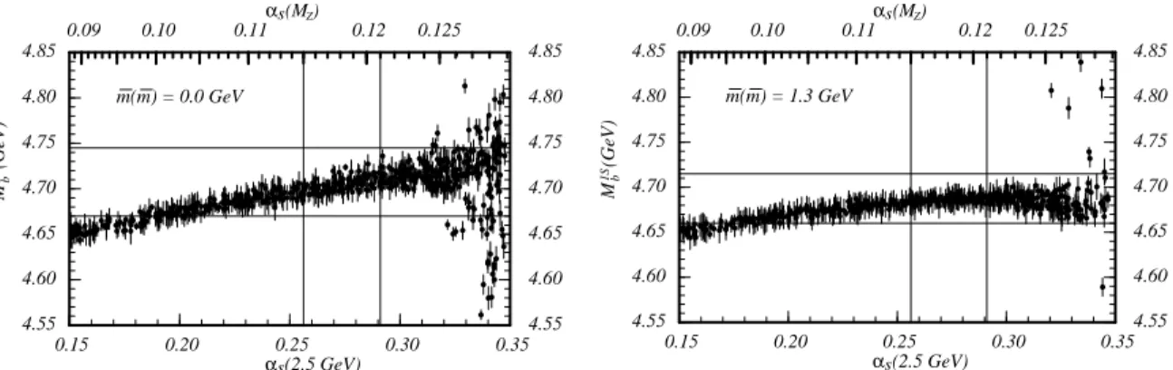
The result for the allowed values for the bottom 1S mass from the χ

-procedure

based on the NNLO theoretical moments is displayed in Fig. 2 for m

(m

) = 0.0 and

1.3 GeV. The dots represent points of minimal χ

for a large number of random choices

of renormalization scales and sets of n’s for given values of α

(M

). Experimental

errors at 95% CL are displayed as vertical lines. (See Ref. [5] for more details.)

The dependence of the 1S mass on the input value for α

(M

) turns out to be

quite weak, particularly if the charm mass corrections are taken into account. For

0.15 0.20 0.25 0.30 0.35 αs(2.5 GeV)

4.55 4.60 4.65 4.70 4.75 4.80 4.85

Mb1S(GeV)

0.09 0.10 0.11 0.12 0.125

αs(M )Z

4.55 4.60 4.65 4.70 4.75 4.80 4.85 m(m) = 0.0 GeV

_ _

0.15 0.20 0.25 0.30 0.35

αs(2.5 GeV) 4.55

4.60 4.65 4.70 4.75 4.80 4.85

Mb1S(GeV)

0.09 0.10 0.11 0.12 0.125

αs(M )Z

4.55 4.60 4.65 4.70 4.75 4.80 4.85 m(m) = 1.3 GeV

_ _

Figure 2: Results for the allowed range of M

b

for given values of α

( M

) at NNLO for m

( m

) = 0 . 0 and 1 . 3 GeV. It is illustrated by the vertical and horizontal lines how the allowed range for M

b

is obtained, if 0 . 115 ≤ α

( M

) ≤ 0 . 121 is taken as an input.

m

(m

) = 1.4 ± 0.3 GeV we obtain

M

= 4.69 ± 0.03 GeV (18)

for the bottom 1S mass. The charm mass corrections shift the 1S mass by about -20 MeV, which is compatible with the crude estimate mentioned above. It is quite interesting that this result is compatible with the determination of the 1S mass from M (Υ(1S)) (see Eq. (15)). The difference to Eq. (15) is that that the central value and the error from the sum rule determination are completely independent of the estimate for the size of the non-perturbative gluon condensate contribution. In this respect the result in Eq. (18) should be considered as more solid than the one in Eq. (15).

Taking the approximation formula (13) we then arrive at

M

(M

) = 4.17 ± 0.05 GeV , (19)

for the bottom MS mass, where we have added quadratically the uncertainties from M

(30 MeV), α

(M

) = 0.118 ± 0.003 (30 MeV), µ = 4.7 ± 3GeV (15 MeV) and m

(m

) = 1.4 ± 0.3 GeV (5 MeV). We note that the charm mass corrections in the Υ sum rules and those in the MS-1S mass relation are additive and lead to an overall shift of about -30 MeV in M

(M

) compared to an analysis where the charm mass is neglected altogether. Thus the charm mass effects are are relevant for the sum rule method, in particular if it should turn out that the perturbative uncertainties in the moments can be decreased in the future.

8 Conclusions

In this talk I have reviewed recent results for light quark mass effects in perturba-

tive bottom quark mass determinations from Υ mesons [4,5]. We find that the effects

of the charm mass are non-negligible in view of the present theoretical uncertainties.

Light quark mass corrections were determined for the 1S-pole mass relation at NNLO, for the MS-pole mass relation at order α

and for the Υ sum rules at NNLO. In the determination of the bottom MS mass, M

(M

), from the mass of the Υ(1S) meson the charm mass corrections shift the value of M

(M

) by about -15 MeV. In the determination of the bottom 1S mass, M

, from the Υ sum rules the charm mass corrections shift the value of M

by about -20 MeV. The overall shift of M

(M

) ob- tained from the Υ sum rule analysis is about -30 MeV. The sign and size of the charm mass corrections shows agreement with a recent unquenched lattice determination of M

(M

) [28].

On the conceptual side light quark mass corrections are interesting because they provide a natural tool to investigate the sensitivity the heavy quark mass definitions to infrared momenta.

Acknowledgments

This work was supported in part by the EU Fourth Framework Program “Training and Mobility of Researchers”, Network “Quantum Chromodynamics and Deep Structure of Elementary Particles”, contract FMRX-CT98-0194 (DG12-MIHT).

References

[1] C. T. Sachrajda, hep-lat/0101003; V. Lubicz, hep-lat/0012003.

[2] G. Dissertori, hep-ex/0010005. A. Brandenburg, P. N. Burrows, D. Muller, N. Oishi and P. Uwer, Phys. Lett. B 468, 168 (1999).

[3] K. Melnikov and A. Yelkhovsky, Phys. Rev. D 59, 114009 (1999); A. H. Hoang, Phys. Rev. D 61, 034005 (2000); M. Beneke and A. Signer, Phys. Lett. B 471, 233 (1999).

[4] A. H. Hoang and A. V. Manohar, Phys. Lett. B 483, 94 (2000).

[5] A. H. Hoang, hep-ph/0008102.

[6] Y. Schroder, Phys. Lett. B 447, 321 (1999); M. Peter, Phys. Rev. Lett. 78, 602 (1997).

[7] M. Melles, Phys. Rev. D 62, 074019 (2000); Phys. Rev. D 58, 114004 (1998).

[8] A. Pineda and F. J. Yndurain, Phys. Rev. D 58, 094022 (1998); S. Titard and F. J. Yndurain, Phys. Rev. D 49, 6007 (1994).

[9] F. J. Yndurain, Nucl. Phys. Proc. Suppl. 93 , 196 (2001).

[10] A. H. Hoang, M. C. Smith, T. Stelzer and S. Willenbrock, Phys. Rev. D 59, 114014 (1999).

[11] M. Beneke, Phys. Lett. B 434, 115 (1998).

[12] A. H. Hoang and T. Teubner, Phys. Rev. D 60, 114027 (1999).

[13] A. H. Hoang, Z. Ligeti and A. V. Manohar, Phys. Rev. D 59, 074017 (1999);

Phys. Rev. Lett. 82, 277 (1999).

[14] A. H. Hoang et al., Eur. Phys. J. directC 3, 1 (2000).

[15] I. Bigi, M. Shifman, N. Uraltsev and A. Vainshtein, Phys. Rev. D 56, 4017 (1997).

[16] D. Eiras and J. Soto, Phys. Lett. B 491, 101 (2000).

[17] A. Hoang, PhD thesis, University of Karlsruhe, RX-1578 (AACHEN).

[18] N. Gray, D. J. Broadhurst, W. Grafe and K. Schilcher, Z. Phys. C 48, 673 (1990).

[19] K. Melnikov and T. v. Ritbergen, Phys. Lett. B482, 99 (2000). K. G. Chetyrkin and M. Steinhauser, Nucl. Phys. B573, 617 (2000).

[20] M. B. Voloshin, Yad. Fiz. 36, 247 (1982) [Sov. J. Nucl. Phys. 36,1 (1982)];

H. Leutwyler, Phys. Lett. B98, 447 (1981).

[21] M. B. Voloshin, Int. J. Mod. Phys. A10, 2865 (1995).

[22] E. C. Poggio, H. R. Quinn and S. Weinberg, Phys. Rev. D 13, 1958 (1976).

[23] J. H. Kuhn, A. A. Penin and A. A. Pivovarov, Nucl. Phys. B 534, 356 (1998).

[24] A. H. Hoang, Phys. Rev. D 59, 014039 (1999); A. A. Penin and A. A. Pivovarov, Phys. Lett. B 443, 264 (1998); Nucl. Phys. B 549, 217 (1999);

[25] A. H. Hoang, Nucl. Phys. Proc. Suppl. 86, 512 (2000).

[26] M. E. Luke, A. V. Manohar and I. Z. Rothstein, Phys. Rev. D 61, 074025 (2000);

A. V. Manohar and I. W. Stewart, Phys. Rev. D 62, 014033 (2000); Phys. Rev. D 62, 074015 (2000); Phys. Rev. D 63, 054004 (2001). A. H. Hoang, A. V. Manohar and I. W. Stewart, hep-ph/0102257.

[27] A. H. Hoang, A. V. Manohar, I. W. Stewart and T. Teubner, hep-ph/0011254.

[28] V. Gimenez, L. Giusti, G. Martinelli and F. Rapuano, JHEP0003, 018 (2000).