Tests based on simplicial depth for AR (1) models with explosion

SFB 823

Tests based on simplicial

depth for AR (1) models with explosion

Discussion Paper Anne Leucht, Christoph P. Kustosz,

Christine H. Müller

Nr. 34/2014

explosion

Anne Leucht

Technische Universit¨at Braunschweig Institut f¨ur Mathematische Stochastik

Pockelsstr. 14 D-38106 Braunschweig

Germany

E-Mail: a.leucht@tu-bs.de

Christoph P. Kustosz and Christine H. M¨uller^∗ Technische Universit¨at Dortmund

Vogelpothsweg 87 D-44221 Dortmund

Germany

E-mail: kustosz@statistik.tu-dortmund.de, cmueller@statistik.tu-dortmund.de Abstract

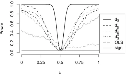
We propose an outlier robust and distributions-free test for the explosive AR(1) model with intercept based on simplicial depth. In this model, simplicial depth reduces to counting the cases where three residuals have alternating signs. Using this, it is shown that the asymp- totic distribution of the test statistic is given by an integrated two-dimensional Gaussian process. Conditions for the consistency of the test are given and the power of the test at finite samples is compared with five alternative tests, using errors with normal distri- bution, contaminated normal distribution, and Fr´echet distribution in a simulation study.

The comparisons show that the new test outperforms all other tests in the case of skewed errors and outliers. Although here we deal with the AR(1) model with intercept only, the asymptotic results hold for any simplicial depth which reduces to alternating signs of three residuals.

2000 Mathematics Subject Classification. Primary 62M10, 62G10; secondary 62G35, 62F05.

Keywords. Alternating signs, autoregression, explosion, distribution-free test, robust- ness, simplicial depth, asymptotic distribution, consistency, power comparison.

Short title. Simplicial depth for AR(1) models.

version: October 7, 2014

∗Research supported by DFG via the Collaborative Research Centre SFB 823 ’Statistical mod- elling of nonlinear dynamic processes’ (Project B5).

1. Introduction Consider the AR(1) model

Y_n =θ₀+θ₁Y_n−1 +E_n, n= 1, . . . , N, (1.1) where E₁, . . . , E_N are i.i.d. errors with med(E_n) = 0, P(E_n= 0) = 0, and Y₀ =y₀ is the starting value. Moreover, it is assumed thatY_nis almost surely strictly increasing, so that Y_n is an exploding process and θ₁ > 1. An example of such an exploding process is crack growth, where a stochastic version of the Paris-Erdogan equation provides Yn = θ1Yn−1 + Een, whereby Een is nonnegative, see Kustosz and M¨uller (2014a). Setting θ0 = med(Een) and En = Een−θ0, we obtain model (1.1) for this case. The aim is to test a hypothesis H₀ : θ = (θ₀, θ₁)^> ∈ Θ₀, where Θ₀ is a subset of [0,∞)×(1,∞). In particular, the aim is to test hypotheses on the median of the distribution of Ee_n as well.

While there is a vast literature on stationary AR(1) models with|θ₁|<1 and for the unit root case with θ₁ = 1, there exist only few results for the explosive case.

Anderson (1959) derived the asymptotic distribution of estimators when the errors E_n are assumed to be independent and normally distributed. Basawa et al. (1989) and Stute and Gr¨under (1993) used bootstrapping methods to derive the asymptotic distribution of estimators and predictors without assuming the normal distribution.

Special maximum likelihood estimators for AR(1) processes with nonnormal errors were treated by Paulaauskas and Rachev (2003). Recently Hwang and Basawa (2005), Hwang et al. (2007) and Hwang (2013) investigated the asymptotic distribution of the least squares estimator of explosive AR(1) processes under some modifications of the process like dependent errors E_n. Further the limit distribution of the Ordinary Least Squares estimator in case of explosive processes was examined by Wang and Yu (2013) and differs from the stationary case depending on the underlying error distribution.

The least squares estimator is known to be sensitive to innovation outliers and additive outliers as discussed in Fox (1972). Outlier robust methods for time series were mainly proposed recently, see e.g. Grossi und Riani (2002), Agostinelli (2003), Fried und Gather (2005), Maronna (2006), Grillenzoni (2009), Gelper et al. (2009).

However these methods deal only with estimation and forecasting. An asymptotic distribution is not derived in these papers so that no tests can be used. Only Huggins (1989) proposed a sign test for stochastic processes based on a M-estimator. The robustness of the sign test was studied in Boldin (2011). Moreover Bazarova et al.

(2014) derived the asymptotic distribution of trimmed sums for AR(1) processes.

However all these approaches base heavily on the stationarity of the process so that they cannot be used for explosive processes.

Here we propose an outlier robust and distribution free test for hypotheses on θ = (θ₀, θ₁)^>for the explosive AR(1) model given by (1.1) which is based on simplicial depth. Simplicial depth was originally introduced by Liu (1988,1990) to provide another generalization of the outlier robust median to multivariate data. The direct generalization of the median to multivariate data is the half-space depth proposed by Tukey (1975). In this definition, the depth of a p-dimensional parameter µwithin

a p-dimensional data set is the minimum relative number of data points lying in a half-space containing the parameter µ. If there are p+ 1 data points then they span a p-dimensional simplex and all points inside the simplex have the half-space depth of 1/(p+ 1) and all points outside the simplex have the depth 0. The simplicial depth of Liu defines the depth of a parameterµas the relative number of simplices spanned by p+ 1 data points which contain the paramter µ, i.e. where the half-space depth of µ with respect to the p+ 1 data points is greater than 0. Replacing the half- space depth by other depth notions leads to a corresponding simplicial depth. For example, Rousseeuw and Hubert (1999) generalized the half-space depth to regression by introducing the concept of nonfit. Thereby the depth of a regression function or respectively the regression parameter θ within a data set is the minimum relative number of data points which must be removed so that the regression function becomes a nonfit. The corresponding simplicial regression depth of ap-dimensional parameter θ is then the relative number of subsets withp+ 1 data points so thatθis not a nonfit with respect to thesep+ 1 data points, see M¨uller (2005). Mizera (2002) proposed a general depth notion by introducing a quality function. Usually the quality function is given by the residuals. Here the residuals of the AR(1) process are used as well.

Simplicial depth has the advantage that it is a U-statistic so that its asymptotic distribution is known in principle. This is usually not the case for the original depth notion. However, the simplicial depth often is a degenerated U-statistic. There are only few cases where this is not the case, see Denecke and M¨uller (2011, 2012, 2013, 2014). For regression problems, the simplicial depth is a degenerated U-statistic.

Deriving the spectral decomposition of the conditional expectation, M¨uller (2005), Wellmann et al. (2009) and Wellmann and M¨uller (2010a,b) derived the asymptotic distribution for several regression problems with independent observations. Only the most simple case, namely linear regression through the origin, can be transferred to AR(1) regression with no intercept θ₀. In this case, the asymptotic distribution is given by one χ²-distributed random variable. This was done in Kustosz and M¨uller (2014a). However, as soon as more than one parameter is unknown, the approaches for an asymptotic distribution developed for regression with independent observations cannot be transferred to autoregression. For example for polynomial regression with independent observations, the asymptotic distribution is given by an infinite sum of χ²-distributed random variables. Here we show, that the asymptotic distribution for the AR(1) model is given by an integrated two-dimensional Gaussian process.

Crucial for this result is that simplicial depth in this model reduces to counting the subsets of three data points where the residuals have alternating signs. Therefore this asymptotic distribution does not hold only for AR(1) models with intercept but also for other models where simplicial depth is given by the number of alternating signs of three residuals. For example it also holds for the nonlinear AR(1) model Y_n =θ₁Y_n−1^θ2 +E_n under similar assumptions as stated above.

In Section 2, we provide the simplicial depth for the AR(1) model with intercept given by (1.1) and the test statistics based on this simplicial depth for hypotheses about θ = (θ₀, θ₁)^>. To obtain the critical values of the tests, the asymptotic distri- bution of the simplicial depth is derived in Section 3. In particular, this asymptotic distribution does not depend on the starting value y₀ of the process as it is the case for the asymptotic distribution of the least squares estimator, see e.g. Hwang (2013).

In Section 4, we derive the consistency of the tests given in Section 2. Although the

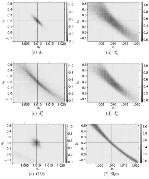
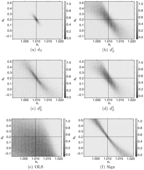
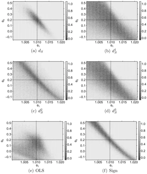
test statistic is given by a very simple form, the calculation of it could be lengthy since all subsets of three observations have to be considered. In Section 5 an efficient algorithm for its calculation is shortly described as well as the efficient calculation of quantiles of the asymptotic distribution. Using this, a power simulation of the new test is given and the power is compared with the power of five other tests, where three of them are based on a simplified version of the depth notion given in Kustosz and M¨uller (2014b).

2. Simplicial depth for the AR(1) model

According to Mizera (2002), we need a quality function to define a depth notion for the AR(1) model (1.1). A natural quality function is the function given by the squared residuals. Set θ= (θ₀, θ₁)^> and define the residuals by

r_n(θ) =y_n−θ₀ −θ₁yn−1, n= 1, . . . , N, where y_n is the realization of Y_n for n= 0, . . . , N.

Tangential depth of the parameterθ in the sampley_∗ = (y₀, . . . , y_N)^> is then (see Mizera 2002)

dT(θ, y∗) = 1 N min

|u|=1]

n ∈ {1, . . . , N}; u^> ∂

∂θrn(θ)² ≤0

so that it becomes d_T(θ, y∗) = 1

N min

|u|=1]

n ∈ {1, . . . , N}; r_n(θ)u^>

1 yn−1

≤0

here. To define simplicial depth for autoregression, it is useful to write the sample in pairs, i.e. the sample is given by z∗ = (z1, . . . , zN)^> where zn = (yn, yn−1)^>. Then, simplicial depth of a p-dimensional parameter θ ∈ R^p in the sample z∗ is in general (see M¨uller 2005)

d_S(θ, z∗) = 1

N p+1

X

1≤n₁<n2<...<np+1≤N

1{d_T(θ,(z_n1, . . . , z_np+1))>0}, where 1{d_T(θ,(z₁, . . . , z_p+1))>0} denotes the indicator function

1A(z₁, . . . , z_p+1) with A={(z₁, . . . , z_p+1)^>∈R^p+1;

d_T(θ,(z₁, . . . , z_p+1))>0}. The simplicial depth is a U-statistic. In the AR(1) model (1.1), it becomes

d_S(θ, z∗) = 1

N 3

X

1≤n₁<n2<n3≤N

1{d_T(θ,(z_n1, z_n2, z_n3))>0}.

If the regressors y_n−1 satisfy y_n1−1 < y_n2−1 < y_n3−1 for n₁ < n₂ < n₃, then d_T(θ,(z_n1, z_n2, z_n3))>0 if and only if the residuals r_n1, r_n2, r_n3 have alternating signs or at least one of them is zero (see Kustosz and M¨uller 2014b). Since Y_n is almost surely strictly increasing by assumption, we can always assumeyn1−1 < yn2−1 < yn3−1

for n1 < n2 < n3 without loss of generality. Moreover, since P(En = 0) = 0, we can restrict ourselve to residuals with alternating signs so that almost surely

d_S(θ, z∗)

= ¹ (^N3)

P

1≤n₁<n2<n3≤N (1{r_n1(θ)>0, r_n2(θ)<0, r_n3(θ)>0}

+1{r_n1(θ)<0, r_n2(θ)>0, r_n3(θ)<0}). If θ is the true parameter, then

d_S(θ, z∗)

= ¹ (^N3)

P

1≤n1<n2<n3≤N (1{e_n1 >0, e_n2 <0, e_n3 >0}

+1{en1 <0, en2 >0, en3 <0}),

wheree_n is the realization of the errorE_n. However, this is not a U-statistic anymore since 1{en1 >0, en2 <0, en3 > 0}+1{en1 <0, en2 >0, en3 < 0} is not a symmetric kernel. Hence, we need the asymptotic distribution for this case which is derived in the next section.

Having the asymptotic distribution of N(d_S(θ, Z∗)− ¹₂) under θ with α-quantile q_α, a simple asymptotic α-level test for the hypothesis H₀ : θ ∈ Θ₀, where Θ₀ is a subset of [0,∞)×(1,∞), is (see M¨uller 2005):

reject H₀ if sup

θ∈Θ₀

N

d_S(θ, z∗)− 1 4

is smaller than q_α, (2.1) i.e. the depths of all parameters of the hypotheses are too small.

3. Asymptotic distribution of the simplicial depth

Even though the statisticd_S(θ, z∗) is not an ordinaryU-statistic due to the lack of symmetry of the kernel, its asymptotics can be obtained similarly to the derivation of of the limit distribution of first-order degenerate U-statistics. First, we define several functions related to the summands of the statistic d_S(θ, z_∗) by

h(x, y, z) = 1{x >0, y <0, z >0}+1{x <0, y >0, z < 0}, (3.1) h₁(x) = Eh(x, E₂, E₃), h₂(y) = Eh(E₁, y, E₃), h₃(z) = Eh(E₁, E₂, z),

h_1,2(x, y) = Eh(x, y, E₃), h_1,3(x, z) = Eh(x, E₂, z), h2,3(y, z) = Eh(E1, y, z).

Note that

h₁(x) = 1

4(1{x <0}+1{x >0}) = 1

4 =h₂(y) =h₃(z) a.s.

which can be compared to first-order degeneracy ofU-statistics since straight-forward calculations yieldvar(h_i,j(E₁, E₂)) = 1/16>0. The latter relations will be important auxiliary results for the derivation of the limit distribution of simplicial depth in the AR(1) setting. Moreover, we will make use of the following approximation.

Lemma 3.1. Under the afore-mentioned assumptions, N

d_S(θ, Z∗)− 1 4

= ^N (^N3)

P

1≤n₁<n2<n3≤N

h1,2(En1, En2) +h1,3(En1, En3) +h_2,3(E_n2, E_n3)− 3

4

+ o_P(1).

Proof. We have to show asymptotic negligibility of N

N 3

X

1≤n₁<n2<n3≤N

h(En1, En2, En3)− 1 4

−

h_1,2(E_n1, E_n2) +h_1,3(E_n1, E_n3) +h_2,3(E_n2, E_n3)− 3 4

.

As the expectation of this quantity is equal to zero, it remains to show that its variance tends to zero as N → ∞. The latter is given by

N²

N 3

2

X

1≤n1<n2<n3≤N

X

1≤¯n1<¯n2<¯n3≤N

E (

h(E_n1, E_n2, E_n3) + 1

2−[h_1,2(E_n1, E_n2) +h_1,3(E_n1, E_n3) +h_2,3(E_n2, E_n3)]

!

× h(E_n¯1, E_¯n2, E_n¯3) + 1

2 −[h_1,2(E_n¯1, E_n¯2) +h1,3(En¯1, En¯3) +h2,3(En¯2, En¯3)]

!) .

The number of summands with n₁ = ¯n₁, n₂ = ¯n₂, n₃ = ¯n₃ is of order O(N³) and therefore the corresponding term asymptotically negligible as the factor in front of the sum is of order O(N⁻⁴). Moreover, note that due to the increasing ordering of the indices it cannot happen that four or more indices coincide. Therefore only three cases remain:

(1) All indices are different from each other.

All these summands are equal to zero by the i.i.d. assumptions on the involved random variables.

(2) Exactly two indices coincide.

Examplarily, we consider the casen1 = ¯n2. All remaining pairs can be treated

in a similar manner and are therefore skipped here. We obtain

E (

h(En1, En2, En3) + 1

2−[h1,2(En1, En2) +h_1,3(E_n1, E_n3) +h_2,3(E_n2, E_n3)]

!

× h(En¯1, En1, En¯3) + 1

2 −[h1,2(En¯1, En1) +h_1,3(E_n¯1, E_n¯3) +h_2,3(E_n1, E_¯n3)]

!)

= E (

(h(En1, En2, En3)−[h1,2(En1, En2) +h1,3(En1, En3)])

× h(E_¯n1, E_n1, E_¯n3) + 1

2−[h_1,2(E_n¯1, E_n1) +h_1,3(E_n¯1, E_n¯3) +h_2,3(E_n1, E_¯n3)]

!)

= E (

h₁(E_n1)h₂(E_n1) + 1

8−h₁(E_n1)h₂(E_n1)− 1

16−h₁(E_n1)h₂(E_n1)

−h₁(E_n1)h₂(E_n1)−1

8 +h₁(E_n1)h₂(E_n1) + 1

16+h₁(E_n1)h₂(E_n1)

−h₁(E_n1)h₂(E_n1)−1

8 +h₁(E_n1)h₂(E_n1) + 1

16+h₁(E_n1)h₂(E_n1) )

= 0,

where the second equality is obtained by conditioning on E_n1 and using the tower property of conditional expectation. The last equality follows from h₁(E_n1)≡h₂(E_n1)≡1/4a.s..

(3) Two pairs of indices coincide.

Examplarily, we consider the case n₁ = ¯n₂, n₂ = ¯n₃. All remaining combi- nations can again be treated in a similar manner and are therefore skipped

here. We proceed as in the previous case and get E

(

h(E_n1, E_n2, E_n3) + 1

2−[h_1,2(E_n1, E_n2) +h1,3(En1, En3) +h2,3(En2, En3)]

!

× h(E_n¯1, E_n1, E_n2) + 1

2 −[h_1,2(E_n¯1, E_n1) +h_1,3(E_¯n1, E_n2) +h_2,3(E_n1, E_n2)]

!)

= E (

h_1,2(E_n1, E_n2)h_2,3(E_n1, E_n2) + 1 8

−h₁(E_n1)h₂(E_n1)−h₂(E_n2)h₃(E_n2)−h_1,2(E_n1, E_n2)h_2,3(E_n1, E_n2)

−h_1,2(E_n1, E_n2)h_2,3(E_n1, E_n2)−1 8

+h₁(E_n1)h₂(E_n1) +h₂(E_n2)h₃(E_n2) +h_1,2(E_n1, E_n2)h_2,3(E_n1, E_n2)

−h₁(E_n1)h₂(E_n1)− 1

8+h₁(E_n1)h₂(E_n1) + 1

16 +h₁(E_n1)h₂(E_n1)

−h2(En2)h3(En2)− 1 8+ 1

16+h2(En2)h3(En2) +h2(En2)h3(En2) )

= 0.

Thus, the variance of the remainder term tends to zero which completes the proof.

In order to derive the asymptotics of N(d_S(θ, Z∗)−1/4) it remains to investigate N

N 3

X

1≤n1<n2<n3≤N

h_1,2(E_n1, E_n2) +h_1,3(E_n1, E_n3) +h_2,3(E_n2, E_n3)− 3 4

= N

2 ^N₃ (

X

1≤n16=n2≤N

(N −max{n₁, n₂})

h_1,2(E_n1, E_n2)−1 4

+ X

1≤n16=n3≤N

(max{n₁, n₃} −min{n₁, n₃} −1)

h_1,3(E_n1, E_n3)−1 4

+ X

1≤n26=n3≤N

(min{n₂, n₃} −1)

h_2,3(E_n2, E_n3)− 1 4

) ,

where we used that h1,2, h1,3, and h2,3, separately, are symmetric.

Now, invoking the fact that

X

1≤n₁6=n₂≤N

min{n1, n2}h1,2(En1, En2) = X

1≤n₂6=n₃≤N

min{n2, n3}h2,3(En2, En3)

and N⁻²P

1≤n₁6=n₂≤N(h1,2(En1, En2) +h1,3(En1, En2)− ¹₂) −→ 0 almost surely with the SLLN, we obtain that the limit distribution of

N(d_S(θ, Z_∗)−1/4) is asymptotically equivalent with

Un= 3 N

X

1≤n₁6=n₂≤N

h1,2(En1, En2)− 1 4

+ 3 N²

X

1≤n16=n2≤N

(max{n₁, n₂} −min{n₁, n₂})

·[h_1,3(E_n1, E_n2)−h_1,2(E_n1, E_n2)].

Now, we invoke a spectral decomposition of the remaining functions in order to separate the the variables E_n1 and E_n2 in a multiplicative manner. The spectral decomposition ofh_1,2−1/4 is provided in Kustosz and M¨uller (2014a, Proof of The- orem 2). The corresponding eigenfunction is given by Φ(x) = 1{x < 0} −1{x > 0}

and the eigenvalue is −1/4. That is h_1,2(x, y)−1/4 = −Φ(x)Φ(y)/4. Similarly, we obtain h_1,3(x, y)−h_1,2(x, y) = Φ(x)Φ(y)/2. Since E[Φ²(E₁)] = 1, the SLLN implies

Un= 3 2N

X

1≤n₁6=n₂≤N

|n₁−n₂|

N − 1

2

Φ(En1)Φ(En2)

= 3 2N

N

X

n1,n2=1

|n₁−n₂|

N − 1

2

Φ(E_n1)Φ(E_n2) + 3

4 +o_P(1).

Even though we separated the involved random variables in a multiplicative manner, the application of a CLT to determine the limit of the first summand is not feasible yet because of the weighting factor |n1−n2|/N −1/2. We solve this problem by a

convolution-based representation of the absolute value function on the interval [-1,1], V_n := 3

2N

N

X

n1,n2=1

|n₁−n₂|

N − 1

2

Φ(E_n1)Φ(E_n2)

= 3 2N

N

X

n1,n2=1

1 2 −

Z ∞

−∞

1^(−0.5,0.5](t)1^(−0.5,0.5]

n₁−n₂

N −t

dt

·Φ(E_n1)Φ(E_n2)

= 3 2N

N

X

n1,n2=1

1 2 −

Z ∞

−∞

1^(−0.5,0.5]n₁ N −t

1^(−0.5,0.5]n₂ N −t

dt

·Φ(E_n1)Φ(E_n2)

= 3 4

√1 N

N

X

n1=1

Φ(E_n1)

!2

− 3 2

Z 2

−2

√1 N

N

X

n1=1

1(−0.5,0.5]

n₁ N −t

Φ(E_n1)

!2

dt To sum up

N

d_S(θ, Z_∗)−1 4

= V_n+3

4 +o_P(1) (3.2)

and the limit distribution of V_n can be deduced by the continuous mapping theorem if the bivariate process

X_N = (X_N,1, X_N,2)^>

=





√1 N

N

X

n1=1

1(−0.5,0.5]

n₁ N −t

Φ(E_n1), 1

√N

N

X

n1=1

Φ(E_n1)

!^>



t∈[−2,2]

converges in distribution to some continuous limiting process with respect to the uniform norm.

Lemma 3.2. Under the assumptions above X_N −→^d X,

where X = (X₁, X₂)^> is a centered Gaussian process on[−2,2]with continuous paths and the covariance structure

Cov(X(s), X(t)) (3.3)

= R1

0 1(−0.5,0.5](x−s)1(−0.5,0.5](x−t) dx R1

0 1(−0.5,0.5](x−s) dx R1

0 1(−0.5,0.5](x−t) dx 1

.

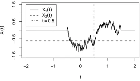
In Figure 1, a simulation of a path of this bivariate process is depicted. The solid line represents the variable X₁(t) which starts in 0 at t =−0.5 and returns to 0 at t = 1.5. The dashed line is a simulation of X2(t). This process is a draw from a

N(0,1) distribution and is constant over time. Note, that the two processes meet at t = 0.5, due to the underlying covariance structure.

−2 −1 0 1 2

−1.5−0.50.51.5

t Xi(t)

X₁(^t)

X2(^t)

t=0.5

Figure 1. Simulation of a path of the limit process

Proof. To prove Lemma 3.2 we apply Theorem 1.5.4 and Problem 1.5.3 in van der Vaart and Wellner (2000) and proceed in several steps.

(1) Convergence of the finite dimensional distributions.

We apply the multivariate Lindeberg-Feller CLT to determine the asymptotics of (XN,1(s1), . . . , XN,1(sk), XN,2(t1), . . . , XN,2(tl)) for arbitrary k, l ∈ N and s1, . . . , sk, t1, . . . , tl ∈ [−2,2]. Obviously, these variables are centered, have finite variance and satisfy the Lindeberg condition. Therefore, it remains to show convergence of the entries of the covariance matrices. For i = 1, . . . , k and j = 1, . . . , l, we get

1 N

N

X

n1=1

var(Φ(En1)) = 1, 1

N

N

X

n1=1

cov

1(−0.5,0.5]

n1

N −t_j

Φ(E_n1),Φ(E_n1)

N→∞−→

Z 1 0

1(−0.5,0.5](x−t_j) dx, 1

N

N

X

n1=1

cov

1^(−0.5,0.5]n₁ N −s_i

Φ(E_n1),1^(−0.5,0.5]n₁ N −t_j

Φ(E_n1)

N→∞−→

Z 1 0

1(−0.5,0.5](x−s_i)1(−0.5,0.5](x−t_j) dx,

in view of EΦ(E1) = 0 and EΦ²(E1) = 1.

(2) A useful moment bound.

For−2≤s ≤t≤2, we obtain using EΦ(E_n1) = 0, EΦ²(E_n1) = 1 = EΦ⁴(E_n1) EkXN(s)−XN(t)k⁴₁

= E 1

√N

N

X

n1=1

Φ(En1)

h1(−0.5,0.5]

n₁ N −s

−1(−0.5,0.5]

n₁ N −t

i

!⁴

= 1

N²

N

X

n1=1

1(−0.5,0.5]

n1

N −s

−1(−0.5,0.5]

n1

N −t

!²

+ 1 N²

N

X

n1=1

h1(−0.5,0.5]

n₁ N −s

−1(−0.5,0.5]

n₁

N −ti4

.

Noting that

1(−0.5,0.5]

n₁ N −s

−1(−0.5,0.5]

n₁ N −t

= 1 for at most 2|t−s|N indices n₁, we end up with

EkX_N(s)−X_N(t)k⁴₁ ≤ 4 (t−s)² + N⁻¹ |t−s|

. (3.4)

(3) Existence and continuity of the limiting process.

By step 1 and Kolmogorov’s existence theorem, there exists a processX with the above-mentioned finite-dimensional distributions. Moreover, from (3.4) we obtain by Fatou’s Lemma

EkX(s)−X(t)k⁴₁ ≤ 4 (t−s)².

Thus, the theorem of Kolmogorov and Chentsov implies that there exists a continuous modification of X that we also refer to asX in the sequel.

(4) Tightness.

By van der Vaart and Wellner (2000, Theorem 1.5.6) it remains to show that for any , η >0 there is a partition −2 =t₀ < t₁ <· · ·< t_K = 2 such that

lim sup

N→∞

P sup

k=1,...,K

sup

s,t∈[tk−1,t_k]

|X_N,1(s)−X_N,1(t)|>

!

≤η

since tightness of (XN,2)N is trivial.

ForXN,1 we obtain

P sup

k=1,...,K

sup

s,t∈[t_k−1,tk]

|X_N,1(s)−X_N,1(t)|>

!

≤2

K

X

k=1

P sup

t∈[tk−1,t_k]

|X_N,1(tk−1)−X_N,1(t)|>

2

!

= 2

K

X

k=1

P sup

t∈[tk−1,t_k]

√1 N

N

X

n1=1

φ(E_n1) (

1(−0.5+tk−1,−0.5+t]

n₁ N

−1(0.5+tk−1,0.5+t]

n₁ N

)

>

2

!

For symmetry reasons we only consider

√1 N

N

X

n1=1

φ(E_n1)1(−0.5+tk−1,−0.5+t]

n₁ N

=Q_N(t)−Q_N(tk−1) with QN(t) := ^√1_N PN

n1=1φ(En1)1(−2,−0.5+t] n1

N

. The process QN has c`adl`ag paths and independent increments. Moreover, note that it follows from the proof of (2) and Markov’s inequality that for some α, β > 0, P(|Q_N(t) − Q_N(s)| ≤ δ) ≥ β whenever |t −s| ≤ α and N ≥ N₀. Therefore we can proceed as in the proof of Theorem V.19 in Pollard (1984) to obtain

lim sup

N→∞

K

X

k=1

P sup

t∈[tk−1,tk]

|Q_N(t)−Q_N(tk−1)|>

4

!

< η 4 for a sufficiently fine equidistant grid.

To sum up, we get the following theorem on the asymptotics of simplicial depth by the continuous mapping theorem.

Theorem 3.1. Under the assumptions above N

dS(θ, Z∗)− 1 4

−→d 3 4 +3

4X₂²(0)− 3 2

Z 2

−2

X₁²(t)dt.

Note, that the asymptotic distribution of the simplicial depth is not restricted to the AR(1) model considered in this paper. It holds for all cases where depth of a two dimensional parameter at three data points is given by alternating signs of the three residuals. This holds in several other models as shown in Kustosz and M¨uller (2014b).

4. Consistency of the tests

Here we show consistency of the test given by (2.1) for hypotheses H₀ : θ = θ⁰ and H0 : θ1 ≥ θ₁⁰ at all relevant alternatives θ^∗ = (θ₀^∗, θ₁^∗)^> by using a large upper bound of the test statistic. Thereby, a test is called consistent at θ^∗ if the power of the test at θ^∗ is converging to one for growing sample size. Hence we have to proof here

N→∞lim P_θ^∗

sup

θ∈Θ₀

N

d_S(θ, Z∗)− 1 4

< q_α

= 1,

where q_α is the α-quantile of the asymptotic distribution of N d_S(θ, Z∗)− ¹₄ given by Theorem 3.1.

Lemma 4.1. If there exists N0 ∈N, δ∈(0,¹₄), and a bounded function H :R³ →R with

H(r_n1(θ^∗), r_n2(θ^∗), r_n3(θ^∗)) (4.1)

≥ sup

θ∈Θ0

1{rn1(θ)>0, rn2(θ)<0, rn3(θ)>0}

+1{r_n1(θ)<0, r_n2(θ)>0, r_n3(θ)<0}

!

for all n₁, n₂, n₃ > N₀ and

E_θ^∗ H(r_n1(θ^∗), r_n2(θ^∗), r_n3(θ^∗))

!

< 1

4 −δ, (4.2)

then the test given by (2.1) is consistent at θ^∗.

Proof. Set M₀ ={(n₁, n₂, n₃);n₃ > n₂ > n₁ > N₀}, then sup

θ∈Θ₀

N

d_S(θ, Z∗)−1 4

≤ N

N 3

X

1≤n1<n2<n3≤N

sup

θ∈Θ0

(1{r_n1(θ)>0, r_n2(θ)<0, r_n3(θ)>0}

+ 1{r_n1(θ)<0, r_n2(θ)>0, r_n3(θ)<0})− 1 4

≤ N

N 3

N 3

−

N −N0

3

+ X

(n1,n2,n3)∈M₀

H(r_n1(θ^∗), r_n2(θ^∗), r_n3(θ^∗))− 1 4

=:T.

Hence, we will work withT. To apply Chebyshev’s inequality, we need upper bounds for the expectation and the variance ofT. Since (4.2) holds onM0 and the indicators

are bounded on the remaining indices, we get

E_θ^∗(T)≤ N

N 3

N 3

−

N −N₀ 3

+

N −N₀ 3

(−δ)

! .

Then there exists N₁ > N₀ such that 1

N 3

N −N₀ 3

≥1−δ and 1

N 3

N

3

−

N −N₀ 3

< δ 2 for all N ≥N₁ implying

E_θ^∗(T)≤N δ

2 + (1−δ)(−δ)

=−N δ₀

with δ₀ = ¹₂δ−δ² >0 since δ < ¹₄. Setting

H_n1,n2,n3 = H(r_n1(θ^∗), r_n2(θ^∗), r_n3(θ^∗))−E_θ^∗[H(r_n1(θ^∗), r_n2(θ^∗), r_n3(θ^∗))], we obtain for the variance

var_θ^∗(T) = N²

N 3

2E_θ^∗ (



X

(n1,n2,n3)∈M₀

H_n1,n2,n3





2)

= N²

N 3

2

X

(n1,n2,n3)∈M0

X

(n1,n2,n3)∈M0

E_θ^∗ H_n1,n2,n3 H_n1,n2,n3

! .

For ^N−N₃ ⁰ _N−N0−3

3

combinations, all n₁, n₂, n₃ are different from n₁, n₂, n₃, so that the independence of the residuals r_n(θ^∗) implies

E_θ^∗(H_n1,n2,n3 H_n1,n2,n3) = 0 for these cases. In all other cases, Eθ^∗(Hn1,n2,n3 Hn1,n2,n3) is bounded by someb² so that

var_θ^∗(T)≤ N²

N 3

2

N−N0

3 2

−

N −N0

3

N −N0−3 3

! b².

Hence for all >0, there exists N₂ ≥N₁ > N₀ such that δ₀ +_N^qα

2 >0 and varθ^∗(T)≤N²

δ0+ q_α N₂

2

for all N ≥ N2. Finally, Chebyshev’s inequality provides for all N ≥ N2 using

qα

N ≥ _N^qα

2

P_θ^∗

sup

θ∈Θ0

N

d_S(θ, Z∗)− 1 4

≥q_α

≤ Pθ^∗ T ≥qα

!

≤Pθ^∗ |T −Eθ^∗(T)| ≥qα−Eθ^∗(T)

!

≤ P_θ^∗ |T −E_θ^∗(T)| ≥q_α+N δ₀

!

≤

N²

δ₀+ _N^qα

2

2

N² δ₀+ ^q_N^α2

≤

δ₀+ _N^qα

2

2

δ₀+_N^qα

2

2 =,

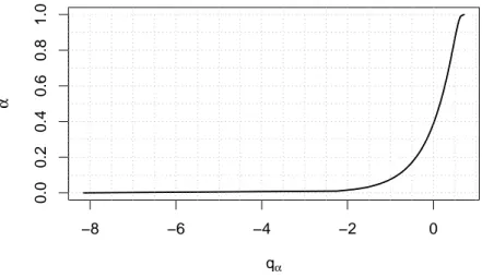
since qα <0 (see Section 5).

The following Lemma is easy to see by induction.

Lemma 4.2. If Y₀ =y₀ and the errors satisfy E_n ≥y₀−θ₀ −θ₁y₀+c for all n for some y₀ >0 and c > 0, then Y_n is strictly increasing with

Y_n≥

n−1

X

k=0

θ₁^k

!

c+y₀.

If, for example, the errors have a shifted Fr´echet distribution as used in the sim- ulations in Section 5, then E_n ≥ y₀−τ y₀+c and med(E_n) = 0 is satisfied for some y₀ >0, c >0, and τ >1.

Theorem 4.1. If the errors satisfy E_n ≥ y₀ −τ y₀ +c for all n for some y₀ > 0, c >0, τ >1, Y₀ =y₀, Θ = [0,∞)×[τ,∞), θ₀⁰ ≥0, θ₁⁰ > τ and

Θ₀ ={(θ₀, θ₁)^>∈Θ; θ₁ ≥θ₁⁰} or Θ₀ ={(θ⁰₀, θ⁰₁)^>}, then the test given by (2.1) is consistent at all θ^∗ ∈Θ\Θ₀.

Proof. Set Θ^h₀ = {(θ₀, θ₁)^> ∈ Θ; θ₁ ≥ θ⁰₁} for the half-sided null hypotheses and Θ^p₀ ={(θ⁰₀, θ₁⁰)^>} for the point null hypothesis and use h defined in (3.1).

Ifθ^∗ ∈Θ\Θ^h₀ then sup

θ∈Θ^h₀

h(rn1(θ), rn2(θ), rn3(θ))

≤ sup

θ∈Θ^h₀

1{r_n1(θ)>0}+1{r_n2(θ)>0}

!

= sup

θ∈Θ^h₀

1{r_n1(θ^∗)> θ₀−θ₀^∗+ (θ₁−θ^∗₁)Y_n1−1}

+1{r_n2(θ^∗)> θ₀−θ^∗₀+ (θ₁−θ^∗₁)Y_n2−1}

!

≤ 1{r_n1(θ^∗)>−θ₀^∗+ (θ₁⁰−θ^∗₁)Y_n1−1} +1{r_n2(θ^∗)>−θ^∗₀+ (θ⁰₁ −θ^∗₁)Y_n2−1}

since θ₀ ≥ 0 and θ₁ ≥ θ⁰₁ for θ = (θ₀, θ₁)^> ∈ Θ^h₀. According to Lemma 4.2, for all γ >0 there exist N0 such that

Y_n ≥

n−1

X

k=0

θ^k₁

!

c+y₀ ≥γ

for all N ≥ N₀. In particular γ can be chosen such that −θ^∗₀ + (θ⁰₁ −θ₁^∗)γ > k and P_θ^∗(r_n(θ^∗)> k)< ¹₂(¹₄ −δ) withδ ∈(0,¹₄) since θ⁰₁ > θ₁^∗. Setting

H(r_n1(θ^∗), r_n2(θ^∗), r_n3(θ^∗)) =1{r_n1(θ^∗)> k}+1{r_n2(θ^∗)> k}, Conditions (4.1) and (4.2) are satisfied, so that consistency holds for all θ^∗ ∈Θ\Θ^h₀.

Ifθ^∗ ∈Θ\Θ^p₀andθ₁⁰ > θ^∗₁, then consistency atθ^∗follows as above. Ifθ⁰₁ < θ₁^∗, then there exists γ > 0 with θ⁰₀ −θ^∗₀ + (θ₁⁰−θ₁^∗)γ <−k and P_θ^∗(r_n(θ^∗)<−k)< ¹₂(¹₄ −δ) so that

H(r_n1(θ^∗), r_n2(θ^∗), r_n3(θ^∗)) =1{r_n1(θ^∗)<−k}+1{r_n2(θ^∗)<−k}

satisfies Conditions (4.1) and (4.2). If θ₁⁰ =θ^∗₁, then k :=θ₀⁰−θ₀^∗ 6= 0 and h(r_n1(θ), r_n2(θ), r_n3(θ))

= 1{r_n1(θ^∗)> k, rn2(θ^∗)< k, rn3(θ^∗)> k}

+1{r_n1(θ^∗)< k, r_n2(θ^∗)> k, r_n3(θ^∗)< k}

=: H(r_n1(θ^∗), r_n2(θ^∗), r_n3(θ^∗)).

Since p(1−p)p+ (1−p)p(1−p) =p(1−p)< ¹₄ for all p6= ¹₂ and

p = Pθ^∗(rn(θ^∗) < k) 6= ¹₂, Condition (4.2) is also satisfied. Hence consistency holds for all θ^∗ ∈Θ\Θ^p₀ as well.