SFB 823
Tests for scale changes based on pairwise differences
Discussion Paper Carina Gerstenberger, Daniel Vogel,
Martin Wendler
Nr. 82/2016
Tests for scale changes based on pairwise differences
Carina Gerstenberger, Daniel Vogel, and Martin Wendler November 13, 2016
In many applications it is important to know whether the amount of fluctuation in a series of observations changes over time. In this article, we investigate different tests for detecting change in the scale of mean-stationary time series. The classical approach based on the CUSUM test applied to the squared centered, is very vulnerable to outliers and impractical for heavy-tailed data, which leads us to contemplate test statistics based on alternative, less outlier-sensitive scale estimators.
It turns out that the tests based on Gini’s mean difference (the average of all pairwise distances) or generalizedQnestimators (sample quantiles of all pairwise distances) are very suitable candidates. They improve upon the classical test not only under heavy tails or in the presence of outliers, but also under normality. An explanation for this counterintuitive result is that the corresponding long-run variance estimates are less affected by a scale change than in the case of the sample-variance-based test.
We use recent results on the process convergence of U-statistics and U-quantiles for dependent sequences to derive the limiting distribution of the test statistics and propose estimators for the long-run variance. We perform a simulation study to investigate the finite sample behavior of the tests and their power. Furthermore, we demonstrate the applicability of the new change-point detection methods at two real-life data examples from hydrology and finance.
Keywords: Asymptotic relative efficiency, Change-point analysis, Gini’s mean dif- ference, Long-run variance estimation, Median absolute deviation, Q
nscale estimator, U-quantile, U-statistic
1. Introduction
The established approach to testing for changes in the scale of a univariate time series X
1, . . . , X
nis a CUSUM test applied to the squares of the centered observations, which may be written as
T ˆ
σ2= max
1≤k≤n
√
k n
σ ˆ
21:k−σ ˆ
1:n2, (1)
where ˆ σ
i:j2denotes the sample variance computed from the observations X
i, . . . , X
j,
1
≤i < j
≤n. To carry out the test in practice, the test statistic is usually divided by
(the square root of) a suitable estimator of the corresponding long-run variance, cf. (8).
This has first been considered by Inclan and Tiao (1994), who derive asymptotics for centered, normal, i.i.d. data. It has subsequently been extended by several authors to broader situations, e.g., Gombay et al. (1996) allow the mean to be unknown and also propose a weighted version of the testing procedure, Lee and Park (2001) extend it to linear processes, and Wied et al. (2012) study the test for sequences that are L
2NED on α-mixing processes. A multivariate version was considered by Aue et al. (2009).
The test statistic (1) is prone to outliers. This has already been remarked by Inclan and Tiao (1994) and has led Lee and Park (2001) to consider a version of the test using trimmed observations. Outliers may affect the test decision in both directions: A single outlier suffices to make the test reject the null hypothesis at an otherwise stationary sequence, but more often one finds that outliers mask a change, and the test is generally very inefficient at heavy-tailed population distributions. An intuitive explanation is that, while outliers blow up the test statistic ˆ T
σ2, they do even more so blow up the long-run variance estimate, by which the test statistic is divided.
1Writing the test statistic as in (1) suggests this behavior may be largely attributed to the use of the sample variance as a scale estimator. The recognition of the extreme
“non-robustness” of the sample variance and derived methods, in fact, stood at the beginning of the development of the area of robust statistics as a whole (e.g. Box, 1953;
Tukey, 1960). Thus, an intuitive way of constructing robust scale change-point tests is to replace the sample variance in (1) by an alternative scale measure.
We consider several popular scale estimators: the mean absolute deviation, the median absolute deviation (MAD), the mean of all pairwise differences (Gini’s mean difference) and sample quantiles of all pairwise differences. All of them allow an explicit formula and are computable in a finite number of steps. Particularly the latter two, the mean as well as sample quantiles of the pairwise differences are promising candidates as they are almost as efficient as the standard deviation at normality and, hence, the improvement in robustness is expected to come at practically no loss in terms of power under normality.
In fact, as it turns out, these tests can have a better power than the variance-based test also under normality.
The paper is organized as follows: In Section 2 we review the properties of the scale estimators and detail on our choice to particularly consider pairwise-difference-based estimators. Section 3 states the test statistics and long-run variance estimators and contains asymptotic results. Section 4 addresses the question which sample quantile of the pairwise differences is most appropriate for the change-point problem. Section 5 presents simulation results. Section 6 illustrates the behavior of the tests at informative real-life data examples. We draw our conclusions in Section 7. Appendix A contains supplementary material for Section 4. Proofs are deferred to the Appendix B.
1This applies in principle to any estimation method, bootstrapping or subsampling, not only to the kernel estimation method employed in the present article.
2. Scale Estimators
We use
L(X) to denote thelaw, i.e., the distribution, of any random variable X. We call any function s :
F →[0,
∞], where Fis the set of all univariate distributions F, a scale measure (or, analogously, a dispersion measure) if it satisfies
s(L(aX + b)) =
|a|s(L(X))for all a, b
∈R. (2) Although not being a scale measure itself, the variance σ
2= E(X
−EX)2is, in a lax use of the term, often referred to as such, since it is closely related to the standard deviation σ =
√σ
2, which is a proper scale measure in the above sense. A scale estimator s
nis then generally understood as the scale measure s applied to the empirical distribution F
ncorresponding to the data set
Xn= (X
1, . . . , X
n). However, it is common in many situations to define the finite-sample version of the scale measure slightly different, due to various reasons. For instance, the sample variance σ
2n=
{(n−1)
−1Pni=1
(X
i−X ¯
n)
2}1/2has the factor (n
−1)
−1due to the thus obtained unbiasedness.
A concept that we will refer to repeatedly throughout is asymptotic relative efficiency.
Letting s
nbe a scale estimator and s the corresponding population value, the asymptotic variance ASV (s
n) = ASV (s
n; F) of s
nat the distribution F is defined as the variance of the limiting normal distribution of
√n(s
n−s), when s
nis evaluated at an independent sample X
1, . . . , X
ndrawn from F . Generally, for two consistent estimators a
nand b
nestimating the same quantity θ
∈R, i.e., a
n−→p
θ and b
n−→p
θ, the asymptotic relative efficiency of a
nwith respect to b
nat distribution F is defined as
ARE(a
n, b
n; F ) = ASV (b
n; F )/ASV (a
n; F ).
In order to make two scale estimators s
(1)nand s
(2)ncomparable efficiency-wise, we have to normalize them appropriately, and define their asymptotic relative efficiency at the population distribution F as
ARE(s
(1)n, s
(2)n; F ) = ASV (s
(2)n; F) ASV (s
(1)n; F)
(
s
(1)(F ) s
(2)(F )
)2
, (3)
where s
(1)(F ) and s
(2)(F ) denote the corresponding population values of the scale esti- mators s
(1)nand s
(2)n, respectively.
In the following, we review some basic properties of four scale estimators: the mean deviation, the median absolute deviation (MAD), Gini’s mean difference and the Q
nscale estimator proposed by Rousseeuw and Croux (1992).
Let md (F ) denote the median of the distribution F , i.e., the center point of the interval
{x ∈ R|F(x−)
≤1/2
≤F (x)}, where F (x−) denotes the left-hand limit.
We define the mean deviation as d(F ) = E|X
−md(F )| and its empirical version as d
n=
n−11 Pni=1|Xi−
md(F
n)|.
The question of whether to prefer the standard deviation or the mean deviation has
become known as Eddington–Fisher debate. The tentative winner was the standard de-
viation after Fisher (1920) showed that its asymptotic relative efficiency with respect to
the mean deviation is 114% at normality. However, Tukey (1960) pointed out that it is less efficient than the mean deviation if the normal distribution is slightly contaminated.
Thus, the mean deviation appears to be a suitable candidate scale estimator for con- structing less outlier-sensitive change-point tests. Gerstenberger and Vogel (2015) argue that, when pondering the mean deviation instead of the standard deviation for robustness reasons, it may be better to use Gini’s mean difference g
n=
n(n−1)2 P1≤i<j≤n|Xi−
X
j|,i.e., the mean of the absolute distances of all pairs of observations. The population ver- sion is g (F ) = E
|X−Y
|, whereX, Y
∼F are independent. Gini’s mean difference has qualitatively the same robustness under heavy-tailed distributions as the mean devia- tion, but retains an asymptotic relative efficiency with respect to the standard deviation of 98% at the normal distribution (Nair, 1936).
Both estimators, mean deviation and Gini’s mean difference, improve upon the vari- ance and the standard deviation in terms of robustness, but are not robust in a modern understanding of the term. They both have an unbounded influence function and an asymptotic breakdown point of zero. Since robustness is, at least initially, our main motivation, it is natural to consider estimators that have been suggested particularly for that purpose. A common highly robust scale estimator is the median absolute deviation (MAD), popularized by Hampel (1974). The population value m (F ) is the median of the distribution of
|X−md (F )
|and the sample version m
n= m
n(
Xn) is the median of the values
|Xi−md(F
n)|, 1
≤i
≤n. The MAD has a bounded influence function (see Huber and Ronchetti, 2009) and an asymptotic breakdown point of 50%. Its main drawback is its poor asymptotic efficiency under normality, which is only 37% as com- pared to the standard deviation. It is also unsuitable for change-in-scale detection due to other reasons that will be detailed in Sections 4 and 5.
Similarly, to going from the mean absolute deviation to the median absolute deviation, we may consider the median, or more generally any sample α-quantile, of all pairwise differences. We call this estimator Q
αnand the corresponding population scale measure Q
α, i.e. Q
α= U
−1(α) = inf
{x|α
≤U (x)}, where U is the distribution function of
|X−Y|
for X, Y
∼F independent, and U
−1the corresponding quantile function. For the precise definition of Q
αn, any sensible definition of the sample quantile can be employed.
See, e.g., the nine different versions the R function quantile() offers. The asymptotic results we derive later are not affected, and any practical differences turn out to be negligible in the current context. So merely for simplicity, we define Q
αn= U
n−1(α), where U
nis the empirical distribution function associated with the sample
|Xi −X
j|,1
≤i < j
≤n. Thus letting D
1, . . . , D (
n2) be the elements of
{|Xi−X
j| |1
≤i < j
≤n}
in ascending order, we have Q
αn= D
α(
n2) if α
n2is integer and Q
αn= D
dα(
n2)
eotherwise.
2In case of Gini’s mean difference, we observed that the transition from the average distance from the symmetry center to the average pairwise distance led to an increase in efficiency under normality. The effect is even more pronounced for the median distances, we have ARE(Q
0.5n, σ
n, N (0, 1)) = 86.3%. Rousseeuw and Croux (1993) propose to use the lower quartile, i.e., α = 1/4, instead of the median. Specifically, they define the finite-
2Note that the empirical 1/2-quantile in this sense does not generally coincide with the above definition of the sample median.
sample version as the
bn/2c+12th order statistic of the
n2values
|Xi−Xj|, 1≤i < j
≤n.
They call this estimator Q
n, and it’s become known under this name, which leads us to call the generalized version Q
αn. The original Q
nhas an asymptotic relative efficiency with respect to the standard deviation at normality of 82%. Rousseeuw and Croux (1993) settle for the slightly lesser efficiency to achieve the maximal breakdown point of about 50%. However, this aspect is of much lesser relevance in the change-point context, quite the contrary, the very property of high-breakdown-point robustness is counterproductive for detecting change-points. The original Q
nis unsuited as a substitution for the sample variance in (1), and a larger value of roughly 0.7 < α < 0.9 is much more appropriate for the problem at hand. We defer further explanations to Section 4, where we discuss how to choose the α appropriately.
These five scale measures, the standard deviation, the mean deviation d
n, Gini’s mean difference g
n, the median absolute deviation (MAD) m
n, and the α-sample quantile of all pairwise differences Q
αn, are the ones we restrict our attention to in the present article.
They are summarized in Table 1 along with their sample versions. There are of course many more potential scale estimators that satisfy the scale equivariance (2) and more robust proposals in the literature, many of which include a data-adaptive re-weighting of the observations (e.g. Huber and Ronchetti, 2009, Chapter 5). In the present paper we explore the use of these common, easy-to-compute estimators in the change-point setting. They all admit explicit formulas, all can be computed in O(n log n) time, and the pairwise-difference estimators allow computing time savings for sequentially updated estimates (which are required in the change-point setting) – more so than, e.g., implicitly defined estimators. The two pairwise-difference based estimators, the average and the α-quantile of all pairwise differences, possess promising statistical properties. We will mainly focus on these and derive their asymptotic distribution under no change in the following section.
3. Test statistics, long-run variances and asymptotic results
We first describe the data model employed: a very broad class of data generating pro- cesses, incorporating heavy tails and short-range dependence (Section 3.1). We then propose several change-point test statistics based on the scale estimators introduced in the previous section and provide estimates for their long-run variances (Section 3.2).
We show asymptotic results for Gini’s mean difference and the Q
αnbased tests under the null hypothesis (Sections 3.3 and 3.4, respectively) and discuss methods for an optimal bandwidth selection for the long-run variance estimation (Section 3.5).
3.1. The data model
We assume the data X
1, . . . , X
nto follow the model
X
i= λ
iY
i+ µ, 1
≤i
≤n, (4)
Table 1: Scale estimators; md (F ) denotes the median of the distribution F , F
nits empirical distribution function.
Scale Estimator
Population value Sample version
Standard deviation
σ (F) =
{E(X
−EX)
2}1/2σ
n=
n1 n
−1
n
X
i=1
X
i−X ¯
n2o1/2Mean deviation
d (F ) = E
|X−md (F )| d
n= 1 n
−1
n
X
i=1
|Xi−
md(F
n)|
Gini’s mean difference
g (F ) = E
|X−Y
|g
n= 2 n(n
−1)
X
1≤i<j≤n
|Xi−
X
j|Median absolute deviation
m (F ) = md (G); where G
is cdf of
L{|X−md (F )|} m
n= md
|Xi−md(F
n)|
Q
αnQ
α= U
−1(α); where U is cdf of
L{|X−Y
|}Q
αn= U
n−1(α); where U
nis
empirical cdf of
|Xi−X
j|, 1≤i < j≤nwhere Y
1, . . . , Y
nare part of the stationary, median-centered sequence (Y
i)
i∈Z. We want to test the hypothesis
H
0: λ
1= . . . = λ
nagainst the alternative
H
1:
∃k
∈ {1, . . . , n−1} : λ
1= . . . = λ
k6=λ
k+1= . . . = λ
n.
Note that this set-up is completely moment-free. We allow the underlying process to be dependent, more precisely we assume (Y
i)
i∈Z
to be near epoch dependent in probabil- ity on an absolutely regular process. Let us briefly introduce this kind of short-range dependence condition.
Definition 3.1.
1. Let
A,B ⊂ Fbe two σ-fields on the probability space (Ω,
F,P).
We define the absolute regularity coefficient of
Aand
Bby β (A,
B) =E sup
A∈A
|P (A|B)−
P (A)| . 2. Let (Z
n)
n∈Z
be a stationary process. Then the absolute regularity coefficients of (Z
n)
n∈Zare given by
β
k= sup
n∈N
β (σ (Z
1, . . . , Z
n) , σ (Z
n+k, Z
n+k+1, . . .)) . We say that (Z
n)
n∈Z
is absolutely regular, if β
k→0 as k
→ ∞.The model class of absolutely regular processes is a common model for short-range dependence. But it does not include important classes of time series, e.g., not all linear processes. Therefore, we will not study absolutely regular processes themselves, but approximating functionals of such processes. In this situation, L
2near epoch dependent processes are frequently considered. Since we also consider quantile-based estimators with the advantage of moment-freeness, we want to avoid moment assumptions implicitly in the short-range conditions. For this reason, we employ the concept of near epoch dependence in probability, introduced by Dehling et al. (2016). For further information see Dehling et al. (2016, Appendix A).
Definition 3.2.
We call the process (X
n)
n∈Nnear epoch dependent in probability (or short P-NED) on the process (Z
n)
n∈Z
if there is a sequence of approximating constants (a
l)
l∈Nwith a
l →0 as l
→ ∞, a sequence of functionsf
l:
R2l+1 → Rand a non- increasing function Φ : (0,
∞)→(0,
∞)such that
P (|X
0−f
l(Z
−l, . . . , Z
l)| > )
≤a
lΦ () (5) for all l
∈Nand > 0.
The absolute regularity coefficients β
kand the approximating constants a
lwill have to fulfill certain rate conditions that are detailed in Assumption 3.3.
3.2. Change-point test statistics and long-run variance estimates
We test the null hypothesis H
0against the alternative H
1by means of CUSUM-type test statistics of the form
T ˆ
s= max
1≤k≤n
√
k
n
|s1:k−s
1:n|.
Throughout, we use s
nas generic notation for a scale estimator (where we include, for completeness’ sake, the variance), and s
1:kdenotes the estimator applied to X
1, . . . , X
k. Considering, besides the variance, the four scale estimators introduced in the previous section, we have the test statistics ˆ T
σ2, ˆ T
d, ˆ T
g, ˆ T
m, and ˆ T
Q(α) based on the sample variance, the mean deviation, Gini’s mean difference, the median absolute deviation and the Q
αnscale estimator, respectively. Under the null hypothesis, the sequence X
1, . . . , X
nis stationary, and can be thought of as being part of a stationary process (X
i)
i∈Zwith marginal distribution F (i.e., X
i= λY
i+ µ). Then, under suitable regularity conditions (that are specific to the choice of s
n), the test statistic ˆ T
sconverges in distribution to D
ssup
0≤t≤1|B(t)|, whereB is a Brownian bridge. The quantity D
s2is referred to as the long-run variance. It depends on the estimator s
nand the data generating process.
Expressions for the scale estimators considered here are given below. The distribution of sup
0≤t≤1|B(t)| is well known and sometimes referred to as Kolmogorov distribution.
However, D
2sis generally unknown, depends on the distribution of the whole process (X
i)
i∈Zand must be estimated when applying the test in practice.
33Alternatively, bootstrapping can be employed, we take up this discussion in Section 7.
In the following definitions, let X, Y
∼F be independent. The long-run variances corresponding to the scale estimators under consideration are
D
σ22=
∞
X
h=−∞
cov
(X
0−EX
0)
2, (X
h−EX
h)
2D
2d=
∞
X
h=−∞
cov (|X
0−md(F )|,
|Xh−md(F )|) ,
D
g2= 4
∞
X
h=−∞
cov (ϕ(X
0), ϕ(X
h)) , (6)
where ϕ(x) = E
|x−Y
| −g(F ), D
2m= 1
f
Z2(m(F))
∞
X
h=−∞
cov
1{|X0−md(F)|≤m(F)},
1{|Xh−md(F)|≤m(F)},
where f
Zis the density of Z =
|X−md(F )|, and D
Q2(α) = 4
u
2(Q
α(F ))
∞
X
h=−∞
cov (ψ(X
0), ψ(X
h)) , (7) where ψ(x) = P (|x−Y
| ≤Q
α)−α and u(t) is the density associated with the distribution function U (t) = P (|X
−Y
| ≤t) of
|X−Y
|. An intuitive derivation of the expressionsfor D
2gand D
2Q(α) are given in Appendix B.
The following long-run variance estimators follow the construction principle of het- eroscedasticity and autocorrelation consistent (HAC) kernel estimators, for which we use results by de Jong and Davidson (2000). The HAC kernel function (or weight function) W can be quite general, but has to fulfill Assumption 3.1 (a) below, which is basically Assumption 1 of de Jong and Davidson (2000). There is further a bandwidth to choose, which basically determines up to which lag the autocorrelations are included. For con- sistency of the long-run variance estimate, the bandwidth has to fulfill the rate condition of Assumption 3.1 (b).
Assumption 3.1.
(a) The function W : [0,
∞)→[−1, 1] is continuous at 0 and at all but a finite number of points and W (0) = 1. Furthermore,
|W|is dominated by a non-increasing, integrable function and
Z ∞
0
Z ∞
0
W (t) cos (xt) dt
dx <
∞.(b) The bandwidth b
nsatisfies b
n→ ∞as n
→ ∞and b
n/
√n
→0.
We propose the following long-run variance estimators for the three moment-based scale measures: For the variance we take a weighted sum of empirical autocorrelations of the centered squares of the data, i.e.,
D ˆ
σ22=
n−1
X
k=−(n−1)
W
|k|b
n
1 n
n−|k|
X
i=1
(X
i−X ¯
n)
2−σ
2n(X
i+|k|−X ¯
n)
2−σ
2n, (8)
where ¯ X
nand σ
n2denote the sample mean and the sample variance, respectively, com- puted from the whole sample, cf. Table 1. Similar expressions have been considered, e.g., by Gombay et al. (1996), Lee and Park (2001) and Wied et al. (2012). There are, of course, other possibilities regarding the exact definition of the long-run variance estimate (e.g., use factor 1/n or 1/(n
−k)), the choice of which turns out to have an negligible effect. The strongest impact has the choice of the bandwidth b
n(see Section 3.5).
For the mean deviation, we propose D ˆ
d2=
n−1
X
k=−(n−1)
W
|k|b
n1
n
n−|k|
X
i=1
(|X
i−md(F
n)| − d
n)
|Xi+|k|−md(F
n)| − d
n,
where md(F
n) and d
ndenote the sample median and the sample mean deviation, re- spectively, of the whole sample (cf. Table 1). For Gini’s mean difference we consider
D ˆ
2g= 4
n−1
X
k=−(n−1)
W
|k|b
n1 n
n−|k|
X
i=1
ˆ
ϕ
n(X
i) ˆ ϕ
n(X
i+|k|), where
ˆ
ϕ
n(x) = 1 n
n
X
i=1
|x−
X
i| −g
nis an empirical version of ϕ(x) in (6). For the long-run variance estimates for the quantile-based scale measures m
nand Q
αn, we need estimates for the densities f
Zand u, respectively, for which we use kernel density estimates
f ˆ (t) = 1 nh
nn
X
i=1
K
|Xi−
md(F
n)| − t h
n
,
ˆ
u(t) = 2 n(n
−1)h
nX
1≤i<j≤n
K
|Xi−
X
j| −t h
n
.
The density kernel K and the bandwidth h
nhave to fulfill the following conditions.
Assumption 3.2.
Let K :
R → Rbe symmetric (i.e. K(x) = K(−x)), Lipschitz-
continuous function with bounded support which is of bounded variation and integrates
to 1. Let the bandwidth h
nsatisfy h
n→0 and n h
8/3n → ∞,as n
→ ∞.If we were interested in an accurate estimate of the whole density function, the estimate could be further improved by incorporating the fact that its support is the positive half- axis, but since we are only interested in density estimates at one specific point, this is not necessary. Define
D ˆ
m2= 1 f ˆ
Z(m
n)
n−1
X
k=−(n−1)
W
|k|b
n1
n
n−|k|
X
i=1
ξ ˆ
n(X
i) ˆ ξ
n(X
i+|k|)
with
ξ ˆ
n(x) =
1{|x−md(Fn)|≤mn}−1/2, and
D ˆ
Q2(α) = 4 ˆ u(Q
αn)
n−1
X
k=−(n−1)
W
|k|b
n1 n
n−|k|
X
i=1
ψ ˆ
n(X
i) ˆ ψ
n(X
i+|k|) with
ψ ˆ
n(x) = 1 n
n
X
i=1
1{|x−Xi|≤Qαn}−
α.
Keep in mind that in the expressions above, the HAC bandwidth b
nand the ker- nel density bandwidth h
nplay distinctively different roles: b
nincreases as n increases, whereas h
ndecreases to zero. Also, the kernels W and K serve different purposes: W is an HAC-kernel and is scaled such that W (0) = 1, while K is a density kernel and it is scaled such that it integrates to 1.
Below, in Sections 3.3 and 3.4, we give sufficient conditions for the convergence of the studentized test statistics ˆ D
g−1T ˆ
gand ˆ D
−1Q(α) ˆ T
Q(α), respectively, since the corresponding estimators, as outlined in Section 2, exhibit the best statistical properties, and these tests indeed show the best performance, as demonstrated in Section 5. The variance- based test statistic ˆ D
σ−12T ˆ
σ2, or versions of it, has been considered by several authors. It is treated for L
2NED on α-mixing processes by Wied et al. (2012). As for the mean- deviation-based test statistic ˆ D
−1dT ˆ
d, the convergence can be shown by similar techniques as for ˆ D
−1σ2T ˆ
σ2: the same (2 + δ) moment condition as for Gini’s mean difference along with corresponding rate for the short-range dependence conditions (Assumption 3.3) are required. Additionally, a smoothness condition around md(F ) is necessary to account for the estimation of the central location. For the MAD-based test statistic ˆ D
−1mT ˆ
m, no moment conditions are required, but smoothness conditions on F at md(F ) as well as m(F) =
|X−md(F )|, X
∼F . However, it turns out that the MAD does not provide a workable change-point test. Roughly speaking, the estimate is rather coarse, and the convergence to the limit distribution too slow to yield usable critical values. But even for large n or with the use of bootstrapping methods, the test is dominated in terms of power by the other tests considered.
3.3. Gini’s mean difference
We assume the following condition on the data generating process.
Assumption 3.3.
Let (X
i)
i∈Zbe a stationary process that is P NED on an absolutely regular sequence (Z
n)
n∈Z. There is a δ > 0 such that
(a) the P NED approximating constants a
land the absolute regularity coefficients β
ksatisfy
a
lΦ l
−6= O
l
−62+δδas l
→ ∞and
∞
X
k=1
kβ
δ 2+δ
k
<
∞,(9) where Φ is defined in Definition 3.2, and
(b) there is a positive constant M such that E|X
0|2+δ≤M and E
|fl(Z
−l, . . . , Z
l)|
2+δ≤M for all l
∈N.
Then we have the following result about the asymptotic distribution of the test statistic D ˆ
g−1T ˆ
gbased on Gini’s mean difference under the null hypothesis. The proof is given in Appendix B.
Theorem 3.1.
Under Assumptions 3.1, 3.2, and 3.3, we have D ˆ
g−1T ˆ
g −→dsup
0≤λ≤1|B(λ)|, where (B (λ))
0≤λ≤1is a standard Brownian bridge.
3.4. Q
αnSince Q
αnis a quantile-based estimator, we require no moment condition, and it suffices that the short-range dependence condition (9) is satisfied for “δ =
∞”.Assumption 3.4.
Let (X
i)
i∈Zbe a stationary process that is P NED of an absolutely regular sequence (Z
n)
n∈Zsuch that the PNED approximating constants a
land the ab- solute regularity coefficients β
ksatisfy
a
lΦ(l
−6) = O(l
−6) as l
→ ∞and
∞
X
k=1
kβ
k<
∞,where Φ is defined in Definition 3.2.
However, instead of the moment condition we require a smoothness condition on F.
Assumption 3.5.
The distribution F has a Lebesgue density f such that (a) f is bounded,
(b) the support of f , i.e.,
{x|f(x)> 0}, is a connected set, and
(c) the real line can be decomposed in finitely many intervals such that f is continuous and (non-strictly) monotonic on each of them.
We are now ready to state the following result concerning the asymptotic distribution of the Q
αn-based change-point test statistic. The proof is given in Appendix B.
Theorem 3.2.
Under Assumptions 3.1, 3.2, 3.4, and 3.5, we have, for any fixed 0 < α <
1 that D ˆ
Q−1(α) ˆ T
Q(α)
−→dsup
0≤λ≤1|B(λ)|, where (B (λ))
0≤λ≤1is a standard Brownian
bridge.
3.5. Data-adaptive bandwidth selection
The rate conditions of Assumptions 3.1 on the HAC bandwidth b
nto achieve consistency of the long-run variance estimate are rather mild. However, the question remains how to choose b
noptimally for a given sequence of observations of length n. The answer depends on the degree of serial dependence present in the sequence. Loosely speaking, choosing it too small results in a size distortion, choosing it too large will render the tests conservative and less powerful.
A general approach is to assume a parametric time-series model, minimize the mean squared error in terms of the parameters of the model and then plug-in estimates for the parameters. For instance, to estimate the long-run variance of an AR(1) process with auto-correlation parameter ρ Andrews (1991, Section 6) gives an optimal bandwidth of
b
n= 1.447n
1/3
4ρ
2(1
−ρ
2)
21/3
(10) when the Bartlett kernel is used.
When employing alternative methods to estimate the long-run variance, i.e., block sub-sampling or block bootstrap, one faces the similar challenge of selecting an appro- priate blocklength, and techniques that have been derived for data-adaptive blocklength selection may be “borrowed” for bandwidth selection. For instance, Carlstein (1986) obtains a very similar expression as (10) for an optimal blocklength in the AR(1) setting for a block sub-sampling scheme.
Politis and White (2004) (see also Patton et al. (2009)) derive optimal blocklengths for block bootstrap methods and obtain also an expression similar to (10). This technique is adapted, e.g., by Kojadinovic et al. (2015) for a change-point test based on Spear- man’s rho. Furthermore, B¨ ucher and Kojadinovic (2016a) identified the asymptotically optimal blocklength for the multiplier bootstrap of U-statistics and developed a method to estimate it.
All such methods require the estimation of unknown parameters as, e.g., in (10) the autocorrelation. Alongside exploring alternatives to the sample variance for robust scale estimation, it is advisable to consider alternatives to the sample autocorrelation. A recent comparison of robust autocorrelation estimators is given by D¨ urre et al. (2015), who recommend to use Gnanadesikan-Kettenring-type estimators. Such estimates re- quire robust scale estimates, for which also the Q
nhas been proposed (Ma and Genton, 2000).
Hall et al. (1995) have suggested an alternative approach without estimating autocor-
relations: If the rate, but not the constant, in an expression as (10) is known, the block-
length can be chosen by sub-sampling. For U -statistics, the rate is n
1/3in the case of the
Bartlett kernel (Dehling and Wendler, 2010) and n
1/5for flat-top kernels (B¨ ucher and
Kojadinovic, 2016b). Results on the optimal blocklength for quantiles and U-quantiles
are not known to us, but we suspect that the rates for the optimal blocklength are the
same as for partial sums, because our variance estimator uses a linearization.
Table 2: Power of change-point tests at asymptotic 5% level, based on sample vari- ance/Gini’s mean difference/Q
nfor independent, centered normal observations.
Standard deviation changes from 1 in first half to λ in second half.
standard deviationλin second half
sample size 1.0 1.2 1.5 2.0 3.0
n= 60 .04/.04/.44 .04/.07/.32 .12/.24/.18 .23/.51/.06 .36/.82/.01 n= 500 .04/.04/.08 .63/.64/.52 1/1/1 1/1/1 1/1/1
4. The choice of α for Q
αnIn this section, we address the question which α to choose best when employing the Q
αnscale estimator. The theoretical U-quantile results of the previous setting apply to Q
αnfor any 0 < α < 1. The original Q
nproposed by Rousseeuw and Croux (1993) corresponds roughly to α = 1/4, which is mainly motivated by breakdown considerations. A high- breakdown-estimator is in fact counterproductive for change-point detection purposes, and higher values of α are more appropriate for the problem at hand. A high-breakdown- point estimator is designed, in some sense, to ignore a large portion of outliers, no matter how they are distributed, spatially or temporarily. The perception of robustness in the change-point setting is conceptually different: we want to safeguard against a few outliers or several but evenly distributed over the observed sequence, as they may be generated by a heavy-tailed distribution. A subsequence of outliers on the other hand, which even exhibits some common characteristics differing from the rest of the data, constitutes a structural change, which we want to detect rather than ignore. To illustrate this point, consider the following example: we have a sample where the first 60% of the observations alternate between 1 and
−1 and the second 40% alternate between 100 and−100. Thisconstitutes a very noticeable change in the scale, but the Q
0.25n-based change-point test of the CUSUM type is not able to detect this change. Similar counter-examples can be constructed for analogous change-point tests which compare the first part to the second part of the sample. However, this very artificial example should not be given to much attention. Any quantile-based method is generally suitable for continuous distributions only.
The point may also be illustrated by Monte Carlo simulation results for continuous distributions. Consider the following data situation: starting from an i.i.d. sequence of standard normal observations, we multiply the second half by some value λ. Table 2 shows rejection frequencies at the asymptotic 5% level based on the original Q
nfor sample sizes n = 60 and n = 500 and several values of λ (bandwidth as in the simulations in Section 5, i.e., b
n= 2n
1/3). The numbers of Table 2 suggest that the original Q
nis very unsuitable for change-point detection in small samples. For n = 60, it strongly exceeds the size, and the power is actually lower under alternatives than under the null.
In principle, when the data is large enough, the Q
0.25nis able to pick up scale changes
in the continuous setting, i.e., the 1/4th quantile of all pairwise differences is larger than
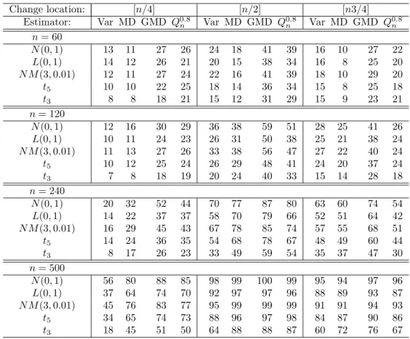
0.0 0.2 0.4 0.6 0.8 1.0 0.0
0.2 0.4 0.6 0.8 1.0
α
ARE
normal Laplace t10
t3
t1
t0.5
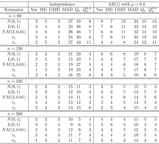
Figure 1: Asymptotic relative efficiencies (AREs) of Q
αnat normal, Laplace, and several t distributions wrt respective maximum-likelihood estimators of scale.
the 1/4th quantile of all pairs of the first half of the observations. For n = 500, this difference is sufficiently pronounced so that the test more or less works satisfactorily.
However, for n = 60, this difference is relatively small compared to the increased long- run variance (by which the test statistic is divided) when λ is large. This largely accounts for the decrease of power as λ increases. Additionally, the Q
n-based test grossly exceeds the size under the null. This can be largely attributed to a general bad “small sample behavior” of the test statistic. We observe a similar effect for the MAD-based test, cf.
Section 5 and the median-based change-point test for location considered by Vogel and Wendler (2016). Thus the Q
0.25nis particularly unsuitable for a quick detection of strong changes.
The problems can be overcome by considering Q
αnfor larger values of α than 1/4, and using such a scale estimator indeed leads to a workable change-point test also for n = 60. As a guideline for a suitable choice of α, we may look at the asymptotic efficiencies. Figure 1 plots the asymptotic relative efficiency of Q
αnat several scale families with respect to the respective maximum-likelihood estimator for scale. The solid line, showing the asymptotic relative efficiency of Q
αnwith respect to the standard deviation at normality, is also depicted in Rousseeuw and Croux (1992). Since we are also interested in efficiency at heavy-tailed distributions, we further include several members of the t
ν- family (for ν = 1/2, 1, 3, 10) and the Laplace distribution, cf. Table 3. The mathematical derivations for this plot, i.e., the asymptotic variances of the Q
αnand the MLE of the scale parameter of the t-distribution, are given in Appendix A.
At normality, the Q
αnis asymptotically most efficient for α = 0.9056 with an asymp-
totic relative efficiency of 99% with respect to the standard deviation, but it shows a
very slow decay as α decreases to zero. For the t-distributions considered, the maximal
asymptotic efficiency of the Q
αnis achieved for smaller values of α, e.g., for the t
3distri- bution, the optimum is attained at α = 0.4661. However, within the range 0 < α < 0.73, the asymptotic relative efficiency with respect to the maximum-likelihood estimator is above 90%. The t
ν-distributions with ν = 1/2 and ν = 1, also depicted in Figure 1, are extremely heavy-tailed. We consider t
νdistributions with ν = 3 and ν = 5 as more realistic data models, and these are also included in the simulation results presented in Section 5.
Altogether, Figure 1 suggests that α
≈3/4 may be a suitable choice as far as asymp- totic efficiency is concerned. We ran simulations with many different values of α and found that Q
αngenerally performed best within the range 0.7 < α < 0.9. In the tables in Section 5, we report results for α = 0.8.
5. Simulation Results
In a simulation study we want to investigate the empirical size and power of the change- point tests based on the test statistics introduced in Section 3.2. We consider the fol- lowing general model: We assume the process (Y
i)
i∈Zto follow an AR(1) process
Y
i= ρY
i−1+
i, i
∈Z,
for some
−1< ρ < 1 where the
iare an i.i.d. sequence with a mean-centered distribution.
Then the data X
1, . . . , X
nare generated as X
i=
(
Y
i, 1
≤i
≤ bθnc,λY
i,
bθnc< i
≤n,
for some 0 < θ < 1. Thus we have four parameters, λ, θ, ρ, and n, which regulate the size of the change, the location of the change, the degree of the serial dependence of the sequence and the sample size, respectively. The tables below report results for λ = 1, 1.5, 2, θ = 1/4, 1/2, 3/4, ρ = 0, 0.8 and n = 60, 120, 240, 500. A fifth “parameter”
is the distribution of the
i, for which we consider the standard normal N (0, 1), the standard Laplace L(0, 1), the normal scale mixture N M(γ, ε) with γ = 3, ε = 0.01 and t
ν-distributions with ν = 3 and ν = 5. The densities of these distributions are summarized in Table 3. The latter four of them are, to varying degrees, heavier-tailed than the normal. The normal mixture distribution captures the notion that the majority of the data stems from the normal distribution, except for some small fraction, which stems from a normal distribution with a γ times larger standard deviation. This type of contamination model has been popularized by Tukey (1960), who argues that γ = 3 is a realistic choice in practice, and further pointed out that in this case the mean deviation d
nis more efficient scale estimator than the standard deviation for values of as low as 1%. Concerning the long-run variance estimation, we take the following choices for bandwidths and kernels,
K(t) = 3
4 (1
−t
2)
1[−1,1](t), W(t) = (1
−t
2)
21[−1,1](t), h
n= I
nn
−1/3, b
n= 2n
1/3,
Table 3: Densities of innovation distributions considered in the simulation set-up. B(·,
·)denotes the beta function.
distribution densityf(x) parameters kurtosis
normalN(µ, σ2) 1
√
2πσ2exp
−(x−µ)2 2σ2
µ∈R, σ2>0
0
normal mixture N M(γ, )
√
2πγexp −x2
2γ2
+1−
√ 2π exp
−x2
2
0≤≤1, γ≥1
3(1−)(λ2−1)2 (λ2+ 1−)2
LaplaceL(µ, α) 1 2αexp
−|x−µ|
α
µ∈R, α >0
3
tν √
νB(ν/2,1/2) 1 +x2/ν−ν+12
ν >0 6
ν−4 (ν >4)
where I
ndenotes the sample interquartile range of the data points the kernel density estimator is applied to. The kernel K above is known as Epanechnikov kernel, and W as quartic kernel. The results of the long-run variance estimation generally differ very little with respect to the choice of kernels. The HAC-bandwidth b
ntends to have the largest influence. We fix it in our simulations to b
n= 2n
1/3, which is large enough to account for the strong serial dependence setting of ρ = 0.8, but is certainly far from optimal in the independence setting, and the results can be improved upon by using one of the data-adaptive bandwidth selection methods outlined in Section 3.5. However, choosing the same, albeit fixed, bandwidth for all change-point tests allows a fair comparison and puts the focus on the impact of the different estimators.
For each setting we generate 1000 repetitions. Tables 4–8 report empirical rejection frequencies (in %) at the asymptotic 5% significance level, i.e., we count how often the test statistics exceed 1.358, i.e., the 95%-quantile of the limiting distribution of the studentized test statistics under the null.
Analysis of size.
Table 4 reports rejection frequencies of the change-point tests based on the variance σ
2n(Var), the mean deviation d
n(MD), Gini’s mean difference g
n(GMD), the median absolute deviation m
n(MAD), the original Q
nas considered by Rousseeuw and Croux (1993), i.e., the
bn/2c+12-th order statistic of all pairwise differences, and the Q
0.8n, i.e., the 0.8
n2-th order statistic of all pairwise differences. We notice that
the Q
nand the MAD heavily exceed the size. This effect wears off as n increases, but
rather slowly. The Q
nshows an acceptable size behavior for n = 500, the MAD not
even for this sample size. This behavior can be attributed to a discretization effect. A
similar observations is made at the median-based change-point test for location, which is
discussed in detail in Vogel and Wendler (2016, Section 4). Due to the size distortion, the
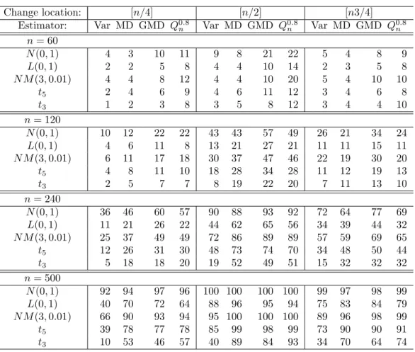
Table 4: Test size. Rejection frequencies (%) of change-point tests based on six different scale estimators at stationary sequences. Asymptotic 5% significance level;
sample sizes n = 60, 120, 240, 500; five different innovation distributions. HAC bandwidth for long-run variance estimation: b
n= 2n
1/3.
independence AR(1) withρ= 0.8 Estimator Var MD GMD MAD Qn Q0.8n Var MD GMD MAD Qn Q0.8n
n= 60
N(0,1) 3 5 3 27 43 6 8 7 13 24 15 14
L(0,1) 3 4 3 23 38 8 7 6 11 23 12 12
N M(3,0.01) 4 6 4 26 46 7 6 6 11 22 14 10
t5 3 4 1 24 40 8 7 6 11 23 13 13
t3 2 5 2 27 43 11 4 4 8 24 12 11
n= 120
N(0,1) 3 3 3 21 29 4 6 6 8 19 8 7
L(0,1) 2 2 2 15 23 5 3 4 7 17 7 7
N M(3,0.01) 2 2 2 19 27 4 4 4 6 18 8 7
t5 1 2 2 19 23 4 4 4 7 17 8 7
t3 2 4 2 16 25 8 3 3 5 19 6 6
n= 240
N(0,1) 2 3 2 15 11 2 3 3 5 15 5 4
L(0,1) 2 3 2 12 10 3 3 3 5 13 5 5
N M(3,0.01) 2 3 3 14 11 4 4 4 6 14 5 6
t5 3 4 3 13 12 3 2 4 5 14 5 4
t3 2 3 3 13 13 6 2 3 4 15 4 5
n= 500
N(0,1) 3 3 3 10 5 4 4 4 4 11 5 5
L(0,1) 3 5 4 9 6 5 5 6 5 10 4 4
N M(3,0.01) 2 3 3 12 6 3 4 4 5 12 3 3
t5 3 4 3 11 7 4 4 4 4 10 5 4
t3 1 3 2 11 7 5 3 4 3 12 4 4
MAD and the Q
nare excluded from any further power analysis. The size exceedance also takes places to a lesser degree for the Q
0.8nat n = 60 and for GMD under dependence at n = 60. This must be taken into account when comparing the power under alternatives.
Based on the simulation results for size and power, the Q
0.8ncan be seen to provide a sensible change-point test for scale, but some caution should be taken for sample sizes below n = 100. All other tests keep the size for the situations considered.
Analysis of power.
Tables 5–8 lists empirical rejection frequencies under various alter-
natives. Tables 5 and 6 show results for serial independence (ρ = 0) for change-sizes
λ = 1.5 and λ = 2, respectively. Tables 7 and 8 contain figures for the serial dependence
setting (ρ = 0.8), again for change-sizes λ = 1.5 and λ = 2, respectively. All tables show
results for θ = 1/4, 1/2, and 3/4 and n = 60, 120, 240, and 500. We make the following
observations:
Table 5: Test power. Rejection frequencies (%) at asymptotic 5% level. Change-point tests based on variance (Var), mean deviation (MD), Gini’s mean difference (GMD), and Q
0.8n.
Independent observations; scale changes by factorλ = 1.5. Several sample sizes, marginal distributions, and change locations. HAC bandwidth: b
n= 2n
1/3.
Change location: [n/4] [n/2] [n3/4]
Estimator: Var MD GMD Q0.8n Var MD GMD Q0.8n Var MD GMD Q0.8n n= 60
N(0,1) 4 3 10 11 9 8 21 22 5 4 8 9
L(0,1) 2 2 5 8 4 4 10 14 2 3 5 8
N M(3,0.01) 4 4 8 12 4 4 10 20 5 4 10 10
t5 2 4 6 9 4 6 11 12 3 4 6 8
t3 1 2 3 8 3 5 8 12 3 4 4 10
n= 120
N(0,1) 10 12 22 22 43 43 57 49 26 21 34 24
L(0,1) 4 6 11 8 13 21 27 21 11 11 15 11
N M(3,0.01) 6 11 17 18 30 37 47 46 22 19 30 20
t5 4 8 11 10 18 28 34 28 11 12 19 13
t3 2 5 7 7 8 19 22 20 7 11 13 10
n= 240
N(0,1) 36 46 60 57 90 88 93 92 72 64 77 69
L(0,1) 11 21 26 22 44 62 65 56 34 39 44 32
N M(3,0.01) 25 37 49 49 72 86 89 89 57 59 69 65
t5 12 26 31 30 48 73 74 70 34 48 50 44
t3 5 18 18 20 19 52 49 51 15 32 32 32
n= 500
N(0,1) 92 94 97 96 100 100 100 100 99 97 98 99
L(0,1) 40 70 72 64 88 96 95 94 75 83 84 79
N M(3,0.01) 66 90 93 94 95 100 100 100 89 96 98 99
t5 39 78 77 78 85 99 98 99 73 90 90 91
t3 10 53 46 57 40 89 84 93 34 70 64 74
(1) All tests have better power at independent sequences than dependent sequences.
Note that ρ = 0.8 constitutes a scenario of rather strong serial dependence.
(2) All tests loose power as the tails of the innovation distribution increase, but the loss is much more pronounced for the variance than for the other estimators. The distributions listed in the tables are in ascending order according to their kurtosis.
The kurtoses of N (0, 1), N M (3, 1%), L(0, 1), t
5, and t
3are 0, 1.63, 3, 6, and
∞,respectively. General formulae are given in Table 3.
(3) The tests generally have a higher power for θ = 3/4 than for θ = 1/4. This may seem
odd at first glance since in both cases the change occurs equally far away from the
center of the sequence. However, since we always consider changes from a smaller
(λ = 1) to a larger scale (λ = 1.5 or 2), a sequence with θ = 1/4 has a higher overall
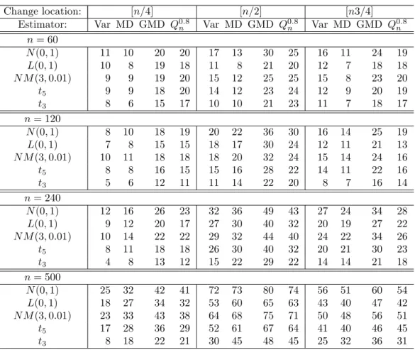
Table 6: Test power. Rejection frequencies (%) at asymptotic 5% level. Same set-up as Table 5 except scale changes by
factorλ = 2.0.
Change location: [n/4] [n/2] [n3/4]
Estimator: Var MD GMD Q0.8n Var MD GMD Q0.8n Var MD GMD Q0.8n n= 60
N(0,1) 2 4 18 21 18 18 46 39 7 5 14 9
L(0,1) 1 1 7 12 7 8 21 22 5 3 8 10
N M(3,0.01) 3 4 16 21 15 16 40 32 6 4 14 9
t5 2 3 9 12 8 12 29 24 4 3 8 11
t3 1 2 5 10 5 7 18 19 4 3 8 12
n= 120
N(0,1) 17 27 53 52 79 86 94 84 58 57 75 40
L(0,1) 6 11 22 22 34 58 68 47 25 30 42 20
N M(3,0.01) 11 20 43 45 65 80 88 81 47 49 66 37
t5 6 14 26 26 43 68 75 63 31 40 49 28
t3 3 8 14 16 18 46 51 45 15 29 35 22
n= 240
N(0,1) 72 89 97 94 100 100 100 100 99 99 100 98
L(0,1) 24 57 66 54 86 98 98 94 76 86 89 77
N M(3,0.01) 52 83 92 92 94 100 100 100 91 98 99 97
t5 26 70 76 77 85 99 99 98 77 92 93 90
t3 9 45 45 49 46 92 89 94 43 76 75 78
n= 500
N(0,1) 100 100 100 100 100 100 100 100 100 100 100 100 L(0,1) 81 100 100 98 100 100 100 100 99 100 100 100 N M(3,0.01) 91 100 100 100 100 100 100 100 100 100 100 100 t5 76 100 100 100 98 100 100 100 97 100 100 100
t3 30 94 89 98 75 100 99 100 72 98 98 100