An adaptive test for the two-sample location problem based on U-statistics
Wolfgang K¨ossler and Narinder Kumar
Humboldt-Universit¨at zu Berlin Panjab University Chandigarh
Abstract
For the two-sample location problem we consider a general class of tests, all members of it are based on U-statistics. The asymp- totic efficicacies are investigated in detail. We construct an adaptive test where all statistics involved are suitably chosen U-statistics. It is shown the adaptive test proposed has good asymptotic and finite power properties.
Keywords: Wilcoxon-Mann-Whitney test, asymptotic efficacy, asymptotic power, simulation study, tailweight, skewness.
1 Introduction
LetX1, . . . , Xn1 andY1, . . . , Yn2 be independent random samples from popu- lations with absolutely continuous distribution functionsF(x) and F(x−ϑ), ϑ ∈R, respectively. We wish to test
H0 : ϑ = 0 against
H1 : ϑ >0.
The Wilcoxon-Mann-Whitney test is the most familiar nonparametric test for this problem. It was generalized to linear rank tests with various other scores, such as the Median test, the normal scores test and the Savage test are proposed, see e.g. H´ajek, ˇSidak and Sen (1999).
Another generalization is to consider a class of tests based on U-statistics.
This interesting class of tests has been attached considerable attraction in the literature (cf. e.g. Deshpande and Kochar (1982), Shetty and Govindarajulu (1988), Kumar (1997), Xie and Priebe (2000)).
Following Kumar, Singh and ¨Ozt¨urk (2003) a general class Uk,i of U- statistics is defined in Section 2. Local alternatives of the form ϑ = θN = θ/√
N,N =n1+n2, are considered and the asymptotic efficacies of the tests based on Uk,i are compared detailly in Section 3. It is shown that there are different tests of this type which are efficient for densities with short, medium or long (right or left) tails, respectively. For example, the test based on U5,1
is efficient for densities with short tails, and that based onU5,3 is efficient for densities with long tails. However, the practising statistician has generally no clear idea on the underlying density, thus he/she should apply an adaptive test which takes into account the given data set. In Sections 4 and 5 two versions of such an adaptive test are proposed, one of them is distribution- free. The adaptive tests first classify the underlying distribution with respect to some measures like (right and left) tailweight and skewness and then select an appropriate test based on U-statistics. In Section 6 a simulation study is performed and the finite power is compared with the asymptotic power. It is shown that one of the adaptive tests behaves well also for moderate sample sizes.
2 Test statistics
We consider the class of U-statistics, which was proposed by Kumar, Singh and ¨Ozt¨urk (2003). Let k and i be fixed integers such that 1 ≤ i ≤ k ≤ min(n1, n2). Define
Φi(x1, . . . , xk, y1, . . . , yk) =
2 if x(i)k < y(i)k and x(k−i+1)k < y(k−i+1)k
1 if either x(i)k < y(i)k or x(k−i+1)k < y(k−i+1)k
0 otherwise,
where x(i)k is the ith order statistic in a subsample of size k from the X- sample (and likewise for y’s). Let Uk,i be the U-statistic associated with kernel Φi, i.e.
Uk,i= n1n2
n1 k
· nk2
XΦi(Xr1, . . . , Xrk, Ys1, . . . , Ysk)−n1n2,
where the summation extends over all possible combinations (r1, . . . , rk) of k integers from {1, . . . , n1} and all possible combinations (s1, . . . , sk) of k integers from {1, . . . , n2}. The null hypothesisH0 is rejected in favour ofH1
for large values of Uk,i.
Remark: The following special cases are of particular interest.
Fori= 1 andk = 1 we have the Wilcoxon-Mann-Whitney test.
Fori= 1 or i=k we have the Despande-Kochar test (cf. Despande and Kochar, 1982).
Fori= (k+ 1)/2 we have the Kumar-test (cf. Kumar, 1997).
Let
ϕ(i)1,0(x) = EΦi(x, X2, . . . , Xk, Y1, . . . , Yk) ϕ(i)0,1(y) = EΦi(X1, . . . , Xk, y, Y2, . . . , Yk)
ζ1,0(i) = Var(ϕ(i)1,0(X)) ζ0,1(i) = Var(ϕ(i)0,1(Y)),
where E and Var denote the expectation and variance rescpectively. More- over, let F(i)k(.) be the cummulative distribution function of the ith order statistics of a sample of size k.
Proposition 2.1 (cf. Kumar, Singh and ¨Ozt¨urk, 2003) Under assump- tions N → ∞, n1/N →λ, 0< λ <1 the limiting distribution of N1/2(Uk,i− ηk,i)/σk,i is standard normal, where expectation ηk,i = EUk,i and variance σk,i2 =var (Uk,i) have the forms
ηk,i = n1n2
Z ∞
−∞
F(i)k(y)dF(i)k(y−θ) + Z ∞
−∞
F(k−i+1)k(y)dF(k−i+1)k(y−θ)
−n1n2
σk,i2 = n21n22 k2ζ10(i)
λ + k2ζ01(i) 1−λ
.
Remark: Under H0 we have ηk,i = 0 and σk,i2 =n21n22k2 ρk,i
λ(1−λ),
where ρk,i depends on k and i only. The expression for ρk,i is rather long, that is why we do not write it out. It can be found in Kumar, Singh and Ozt¨¨ urk (2003).
3 The asymptotic efficacies
The asymptotic Pitman efficacies AE of the statistics Uk,i under the alterna- tive θN =N−1/2·θ are given by
AE(Uk,i|f) =λ(1−λ)·Ck,i2 (f),
wheref(·) denotes the probability density function belonging to the c.d.f.F(·) and
Ck,i(f) = ( ki i)2 (k2ρk,i)1/2 ·
Z ∞
−∞
(F(x))2i−2(1−F(x))2k−2if2(x)dx+
Z ∞
−∞
(F(x))2k−2i(1−F(x))2i−2f2(x)dx
(cf. Kumar, Singh and ¨Ozt¨urk, 2003).
(Note that the asymptotic efficacy is defined by the limit ofηk,i2 /σk,i2 .) To obtain procedures that are practically important also for moderate to small sample sizes we restrict the further investigations to the case of small k, k≤5.
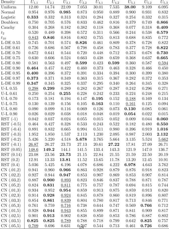
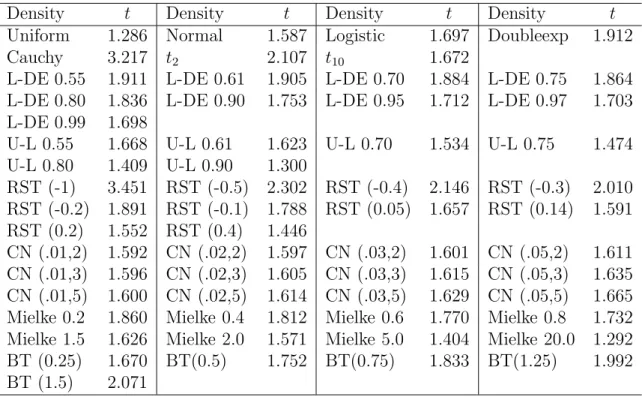
We compute the asymptotic Pitman efficacies for all tests Uk,i with 1 ≤ i≤k,k ≤5. Values of the factors Ck,i2 (f) for various densities are presented in Table 1. The L-DE density was proposed by Policello and Hettmansperger (1976), the U-L by Gastwirth (1965), the RST is named after Ramberg, Schmeiser and Tukey, cf. Ramberg and Schmeiser (1972, 1974), CN(, σ) is the scale contaminated normal with contaminating proportion , Mielke denotes the Mielke (1972) density and BT is the density of Box and Tiao (1962).
The bolded entries denote the, for the given density, asymptotically best test among the considered tests. On the first view we see that the columns for U3,1, U5,1 and U5,3 have the most bolded entries. This observation gives rise to the idea to base an adaptive test on these few statistics. (The classical test U1,1 is also included in the adaptive test.)
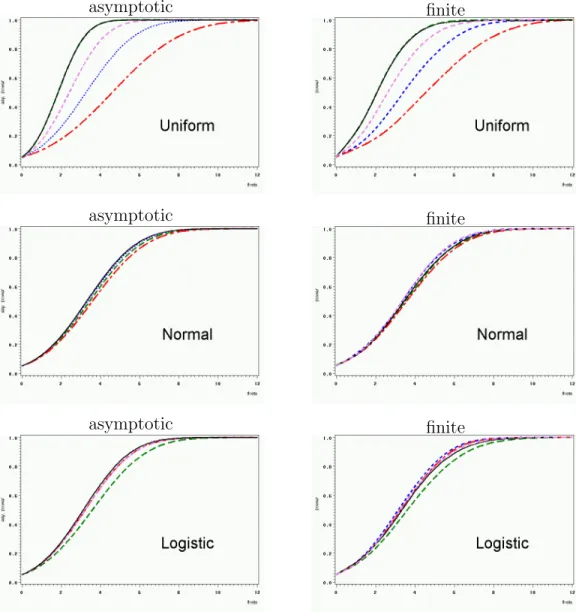
For various densities asymptotic power functions (together with finite power functions) are given in Figures 3 and 4.
The blue dotted line is forU1,1, the violet short-dashed line for U3,1, the green long-dashed line for U5,1, the red dashed-dotted line for U5,3 (and the black continuous line for the adaptive test, see below).
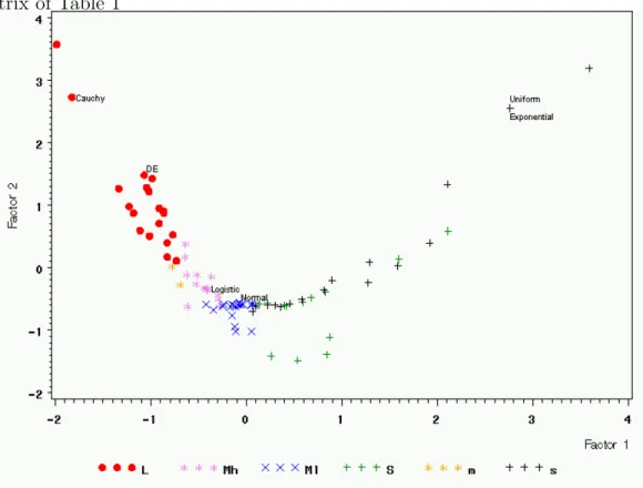
Applying a similar idea of Hall and Joiner (1982) the content of informa- tion in the asymptotic efficacy matrix is analysed by a principal component analysis where the densities are the observations and the efficacies of the Ui,j
are the variables. The first principal component explains already 96% of the variabilty (Figure 1). For better visibility we preferred a two-dimensional plot. In Figure 1 nearly symmetric densities with short tails (S) are denoted by a green plus, that with medium tails (Ml and Mh) by a violet star and a blue X and that with long tails (L) with a red dot. (Ml and Mh stand for medium to light tails and medium to heavy tails respectively.) Skew densities are denoted by a black plus (short tails, s) and a yellow star (medium tails, m) respectively. The dots (L) denote densities with long tails, the stars (M and m) denote densities with medium tails, and the plus (S and s) denote densities with short tails. The small letters (m and s) are for skew densities.
On the left side we have densities with long tails, in the centre that with medium tails, and on the right that with short tails. For an exact definition what we understand by long, medium and short tails see below. On the first view we see that the AE(Uk,i) classify the densities according to their tailweight. The skewness seems to play a marginal role only.
4 Selector statistics
There are some proposals for adaptive tests for the two-sample location prob- lem in the literature, see e.g. Hogg (1974, 1982), Hogg, Fisher and Randles (1975), Ruberg (1986) and B¨uning (1994). We apply the concept of Hogg (1974), that is, to classify at first the type of the underlying density with respect to one measure of skewness ˆs and to three measures of tailweight ˆt,
Figure 1: The first two principal components of the asymptotic efficacy ma- trix of Table 1
tˆr and ˆtl, which are defined by ˆ
s = Q(0.95) + ˆˆ Q(0.05)−2·Q(0.5)ˆ
Q(0.95)ˆ −Q(0.05)ˆ (1)
ˆt = Q(0.95)ˆ −Q(0.05)ˆ
Q(0.85)ˆ −Q(0.15)ˆ (2)
ˆtl = Q(0.5)ˆ −Q(0.05)ˆ
Q(0.5)ˆ −Q(0.15)ˆ ˆtr = Q(0.95)ˆ −Q(0.5)ˆ
Q(0.85)ˆ −Q(0.5)ˆ (3) where ˆQ(u) is the so-called classical quantile estimate of F−1(u),
Q(u) =ˆ
X(1)−(1−δ)·(X(2)−X(1)) if u <1/(2·N) (1−δ)·X(j)+δ·X(j+1) if 2·1N ≤u≤ 2·2N·N−1
X(N)+δ(X(N)−X(N−1)) if u >(2·N−1)/(2·N), (4)
where δ = N ·u+ 1/2−j and j = bN ·u+ 1/2c. Note that ˆtl and ˆtr are measures of left tailweight and right tailweight, respectively.
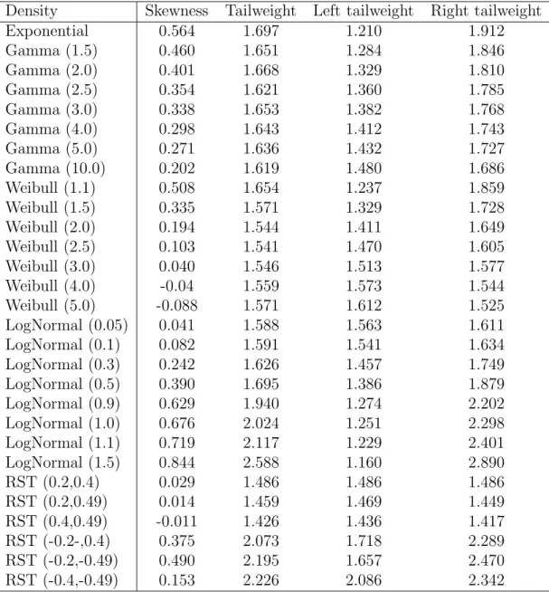
In Tables 2 and 3 the values of the corresponding theoretical measures s, t, tr and tl, for various selected densities are presented. (For symmetric densities we have s= 0 and t=tr =tl.)
Comparing Table 1 with Tables 2 and 3 roughly we see that U5,1 is the asymptotically best test for symmetric densities with small tailweight, U3,1
for symmetric densities with small to medium tailweight, U1,1 for symmetric densities with medium to larger tailweight, and U5,3 for symmetric densities with large tailweight. The testsU3,1 andU1,1 should be included in a adaptive test since they are the (asymptotically) best for the normal and for the logistic density, respectively (at least among the considered tests).
The measure of skewness gives no clear classification idea. That is why we consider left tailweight tl and right tailweight tr, and classify densities as densities with partially short tails if tl < 1.55 or tr < 1.55. They are classified to have partially medium tails if tl < 1.8 or tr < 1.8 and if they have not partially short tails.
5 Presentation of the adaptive test
The reasoning of the last two sections gives rise to the following adaptive test.
Define regions E1, . . . , E7 of R4 which are based on the so called selector statistic ˆS = (ˆs,ˆt,tˆl,tˆr)
E1 ={ˆt <1.55,|sˆ| ≤0.2} “nearly symmetric, short tails” (S)
E2 ={1.55≤ˆt <1.65,|sˆ| ≤0.2} “nearly symmetric, light medium tails” (Ml) E3 ={1.65≤ˆt≤1.8,|sˆ| ≤0.2} “nearly symmetric, heavy medium tails” (Mh) E4 ={ˆt >1.8,|sˆ| ≤0.2} “nearly symmetric, long tails” (L)
E5 ={(ˆtl <1.55 ∨tˆr<1.55),|sˆ|>0.2} “skew, partially short tails” (s) E6 ={(ˆtl >1.65 ∧tˆr>1.65),|sˆ|>0.2} “skew, long tails” (l)
E7 ={ˆtl ≥1.55, ˆtr ≥1.55,|sˆ|>0.2} \E6 “skew, partially medium tails” (m) where ˆs,ˆt,ˆtland ˆtr are given by (1) to (3). Note that there was no density which belongs to class E6.
Looking again at Tables 2 and 3 we see that the vast majority of den- sities is classified correctly, i.e. they fall in that class that has the highest asymptotic power. If the classification is not correct, then the efficacy loss is very small in almost all cases. In Table 1 the chosen test is underlined if it is not already the (bolded) best.
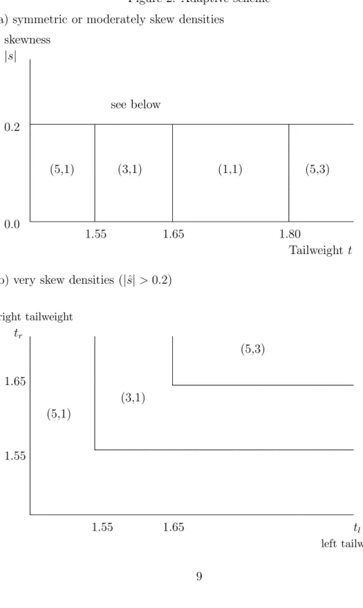
Now, we propose the Adaptive test A which is based on the four U- statistics U5,1, U3,1,U1,1, and U5,3. We denote the tests by (5,1), (3,1), (1,1) and (5,3), respectively.
A=A(S) =
(5,1) if S ∈E1∪E5
(3,1) if S ∈E2∪E7
(1,1) if S ∈E3
(5,3) if S ∈E4∪E6
(5)
In Figure 2 the corresponding adaptive scheme is given. As indicated above the skewness plays only a marginal role. It is included in the adaptive scheme implicitely by left and right tailweight.
The two-stage procedure defined above is asymptoticaly distribution-free since the selector statistic S is based on the order statistic only and the U-statistics are based on the ranks only.
The Adaptive test A is only asymptotically distribution-free because asymptotic critical values are used in the adaptive scheme.
Proposition 5.1 Let σF be the standard deviation of the underlying cdf. F, if it exists and let {θN} be a sequence of ‘near’ alternatives with √
N θN →