On the strength of the U

JHEP12(2016)158

Published for SISSA by Springer

Received: September 1, 2016 Revised: December 9, 2016 Accepted: December 20, 2016 Published: December 30, 2016

On the strength of the U

(1) anomaly at the chiral phase transition in N

= 2 QCD

Bastian B. Brandt,^a,b Anthony Francis,^c Harvey B. Meyer,^d Owe Philipsen,^a Daniel Robaina^d and Hartmut Wittig^d

aInstitut f¨ur Theoretische Physik, Goethe-Universit¨at, D-60438 Frankfurt am Main, Germany

bInstitut f¨ur theoretische Physik, Universit¨at Regensburg, D-93040 Regensburg, Germany

cDepartment of Physics & Astronomy, York University, 4700 Keele St, Toronto, ON M3J 1P3, Canada

dPRISMA Cluster of Excellence, Institut f¨ur Kernphysik and Helmholtz Institut Mainz, Johannes Gutenberg-Universit¨at Mainz, D-55099 Mainz, Germany

E-mail: brandt@th.physik.uni-frankfurt.de,

afrancis.heplat@googlemail.com,meyerh@kph.uni-mainz.de, philipsen@th.physik.uni-frankfurt.de,

robaina@theorie.ikp.physik.tu-darmstadt.de,wittig@kph.uni-mainz.de

Abstract:We study the thermal transition of QCD with two degenerate light flavours by lattice simulations usingO(a)-improved Wilson quarks. Temperature scans are performed at a fixed value ofN_t= (aT)⁻¹= 16, whereais the lattice spacing andT the temperature, at three fixed zero-temperature pion masses between 200 MeV and 540 MeV. In this range we find that the transition is consistent with a broad crossover. As a probe of the restora- tion of chiral symmetry, we study the static screening spectrum. We observe a degeneracy between the transverse isovector vector and axial-vector channels starting from the tran- sition temperature. Particularly striking is the strong reduction of the splitting between isovector scalar and pseudoscalar screening masses around the chiral phase transition by at least a factor of three compared to its value at zero temperature. In fact, the splitting is consistent with zero within our uncertainties. This disfavours a chiral phase transition in theO(4) universality class.

Keywords: Global Symmetries, Lattice QCD, Phase Diagram of QCD, Spontaneous Symmetry Breaking

ArXiv ePrint: 1608.06882

JHEP12(2016)158

Contents

1 Introduction 1

2 Lattice simulations 6

2.1 Simulation and scan setup 6

2.2 Scale setting and lines of constant physics 7

2.3 Observables and renormalisation 7

2.3.1 Deconfinement and the Polyakov loop 7

2.3.2 The chiral condensate 8

2.3.3 Mesonic correlation functions and screening masses 10 2.4 Investigating the order of the transition in the chiral limit 11

2.4.1 Critical scaling 11

2.4.2 U_A(1) symmetry restoration 12

3 Results 12

3.1 Ensembles and measurement setup 12

3.2 The pseudocritical temperature 14

3.2.1 Polyakov loops 14

3.2.2 Chiral condensate and its susceptibility 14

3.2.3 Scaling in the approach to the chiral limit 16 3.3 Screening masses and chiral symmetry restoration pattern 19 3.4 On the relative size of the UA(1) breaking effects around TC 24

4 Conclusions 27

A Simulation and analysis details 28

A.1 Simulation algorithms and associated constraints 28

A.2 Error analysis 29

A.3 Interpolation of zero temperature quantities 30

A.4 Estimating lines of constant physics 31

A.5 Interpolation of the zero temperature chiral condensate 33

B Simulation parameters and results 35

1 Introduction

Nuclear matter under extreme conditions of high temperatures T and/or baryon chemical potential µ_B is the subject of intense experimental and theoretical studies in nuclear, particle and astro-physics. One of the salient features of strongly interacting matter is the

JHEP12(2016)158

high-temperature transition from the hadronic phase to the deconfined quark-gluon plasma (QGP). The transition takes place in a temperature regime between 100 and 300 MeV, where the QCD running coupling is strong. Thus, a non-perturbative investigation of the transition and the properties of the QGP is necessary and a lot of effort has been invested by the lattice community in the past decades (for recent reviews see [1–5]).

Because lattice studies of the QCD transition at finite baryon chemical potentials are severely hampered by the sign problem, the QCD phase diagram remains largely unknown.

Even at zero baryon density, the nature of the thermal transition with light quark masses approaching the chiral limit is not yet determined in the continuum. Knowledge of this important limit would also help to constrain the phase diagram at non-zero µ_B. Figure 1 summarises the current knowledge about the order of the thermal transition for vanishing baryon density in the (m_ud, m_s)-plane, where m_ud is the mass of the degenerate up and down quarks andms the strange quark mass. In the opposite limits of pure gauge theory and QCD with three massless quarks, there are true first-order phase transitions associated with the breaking of centre symmetry [6], and the restoration of the SU(3) chiral symme- try [7], respectively. These get weakened by the explicit breaking of those symmetries by finite fermion masses, until they disappear along second order critical lines. For interme- diate quark masses, the finite temperature transition is then merely an analytic crossover.

There is plenty of evidence that the physical quark mass configuration realised in nature is in the crossover region. Early results based on the staggered fermion discretisation [8,9]

have been confirmed by domain wall fermions [10,11] and simulations with Wilson fermions are approaching the physical point as well [12–15]. The critical line separating the first order chiral transitions from the crossover region, the chiral critical line, has been mapped out on coarse lattices and is in the Z(2) universality class of the 3d Ising model [16,17].

The critical line in the heavy quark region, the deconfinement critical line, is in the same universality class and was mapped out on coarse lattices simulating a hopping expanded determinant [18] and a 3d effective lattice theory [19]. However, the location of the critical lines in the quark mass plane is subject to severe cut-off effects. With standard staggered fermions theN_f = 3 critical pion mass is at around two to three times the physical quark mass [16, 17], yet one finds that it shrinks to nearly half that value when going from N_t= 4 to N_t= 6 [20]. Improved staggered fermions can only give an upper bound for the critical mass which is around 0.1 times the physical quark mass [21,22]. First results with Wilson fermions on the other hand see the N_f = 3 critical endpoint at around five times the physical quark mass [23]. While the latter result will still change when going towards finer lattices, it highlights the importance of taking the continuum limit before discussing critical behaviour.

While all current results indicate that the critical line passes the physical point to the left, its detailed continuation is still largely unknown [2]. There are two possible scenarios [7,24,25]: in scenario (1), depicted in the left panel of figure1, the chiral critical line reaches them_ud= 0 axis at some tri-critical pointm_s=m^tric_s , implying a second order transition forN_f = 2. In the alternative scenario (2) the chiral critical line never reaches them_ud= 0 axis, so that the chiral transition at m_ud= 0 is first order for all values of the strange quark mass.

JHEP12(2016)158

scenario (1): scenario (2):

0 m_s

∞

m_ud N_f = 2

∞ pure gauge

0 m_s

∞

m_ud N_f = 2

∞ pure gauge

N^f

=3

N^f

=3

Nf=1 Nf=1

crossover crossover

1st 1st

2nd

Z(2) 2nd

Z(2)

1st 2nd 1st

Z(2) 2nd

Z(2) m^tric_s

tricrit.

2nd nO(4)?

U(2)?

physical point

physical point

N_f = 2

crossover 1st

2nd 2nd nO(4)? Z(2)

U(2)?

1st crossover 1st

2nd Z(2)

Figure 1. The two possible scenarios for the quark mass dependence of the phase structure of QCD at zero chemical potential. The lower lines highlight the dependence of the phase structure in theNf = 2 case of theuanddquark masses.

Many past studies have investigated the nature of the N_f = 2 transition using stag- gered [26–32], O(a) improved [33–35] or twisted mass [36] Wilson fermions and domain wall and overlap fermions [37–40], without being able to provide a conclusive answer in the chiral limit. The main problem in investigating scaling properties is the similarity of the critical exponents of the universality classes in question (cf. section 2.4.1). A new method to exploit the known tricritical scaling when coming from the plane of imaginary chemical potential has been proposed in [41]. First results on coarse lattices with staggered [42] and Wilson fermions [43] agree on scenario (2), but show enormous quantitative discrepancies.

A similar approach proposed recently is to look at the extension of the chiral critical line in the plane withN_F additional degenerate heavy quarks [44,45].

Which of these scenarios is realised depends crucially on the strength of the anomalous breaking of the UA(1) symmetry at the critical temperature in the chiral limit when the mass of the strange quark is sent to infinity, i.e. in theN_f = 2 case. If the breaking of UA(1) remains strong, the transition will be of second order in the O(4) universality class [7], so that scenario (1) will be realised. If, on the other hand, the symmetry is ‘sufficiently’

restored (see the discussion below about different restoration criteria), either scenario is possible [24,25]. For scenario (1) the breaking would then likely be in the U(2)×U(2)→ U(2) universality class [24, 25] (another symmetry breaking pattern/universality class of the form SU(2)×SU(2) ×Z4 → SU(2) has also been proposed [46, 47]) and the O(4) universality class would be disfavoured. To be able to distinguish between the different

JHEP12(2016)158

scenarios by looking at the U_A(1) symmetry, it is thus crucial to have a measure for the strength of the breaking.

First, we recall that the U_A(1) classical symmetry does not imply the existence of a conserved current: the divergence of the singlet axial current A⁰_µ(x) is proportional to the gluonic operator GG˜ =_µνρσG_µνG_ρσ in the chiral limit, an equality valid in any on-shell correlation function. For instance, the static correlator (∂²/∂x²₃)R

dx₀dx₁dx₂hA⁰₃(x)A⁰₃(0)i is proportional to the corresponding static two-point function of GG, which is certainly˜ non-vanishing at any finite temperature. By contrast, the corresponding two-point function of the non-singlet axial currentA^a₃(x) vanishes in the chiral limit. In this particular sense, the UA(1) symmetry is never restored.

In this paper we use static correlators and the associated screening spectrum to probe the U_A(1) effects. A thermal state with an exactly restored U_A(1) symmetry implies that the correlatorshψ(x)τ¯ ^aψ(x) ¯ψ(0)τ^aψ(0)iandhψ(x)γ¯ 5τ^aψ(x) ¯ψ(0)γ5τ^aψ(0)iare equal in the massless theory. However, we expect the restoration of U_A(1) symmetry in this sense to only be partial, improving as the temperature is increased (see e.g. [48]).

In the literature, the restoration of UA(1) symmetry has also been discussed in a different, more restrictive sense. The observables considered are e.g. the correlation func- tions mentioned in the previous paragraph projected onto zero-momentum (R

d⁴x). Sim- ilar to the Banks-Casher relation for the chiral condensate, the difference of the zero- momentum correlators can be expressed in terms of the spectral density of the Dirac operator alone [49, 50]. For a density ρ(λ) ∼ |λ|^α with α > 1, the difference vanishes exactly in the chiral limit. In such a scenario, it is said that UA(1) symmetry is restored.

More generally, if the SU(2) symmetry is restored at T_C (which we will find to be the case later), the effective restoration of the UA(1) symmetry is indicated by the degener- acy of correlation functions belonging to a U(2)×U(2) multiplet (e.g. [49]). Using the restoration of the SU(2) symmetry, it was shown by Cohen [49,50] that the degeneracy of zero-momentum correlation functions in the multiplets is directly linked to the eigenvalue density ρ(λ) in the vicinity of zero. In particular, if the spectrum of the Dirac operator develops a gap around λ = 0 at T_C, the U_A(1) symmetry becomes effectively restored.

Using QCD inequalities, it has been argued that the UA(1) symmetry is expected to be effectively restored as soon as the SU(2) symmetry is intact [49]. Later it was noted that the result using the inequalities was incorrect since the contributions from sectors with non-zero topology had not been taken into account properly [51, 52]. However, the non- zero topology sectors only contribute away from the thermodynamic limit. Only a bit later it was shown that the eigenvalue density in the chiral limit behaves like ρ(λ)∼ |λ|^α with α >1 [50]. Using mild assumptions and Ward-Takahashi identities for higher order susceptibilities in the framework of overlap fermions on the lattice, it has recently been shown that in fact α > 2 [53], meaning that not only the eigenvalue density, but also its first and second derivative vanish at the origin, speaking strongly in favour of a restoration of the U_A(1) symmetry.

The relation between degeneracy of correlators and the behaviour of the low modes of the Dirac operator triggered a number of numerical studies of the eigenvalue spectrum in the vicinity of T_C [10, 37–40, 54]. Some groups [37, 38] see a restoration of U_A(1) at T in the chiral limit (in particular, in [37] the behaviour of ρ(λ) ∼ |λ|³ was observed),

JHEP12(2016)158

while others claim that U_A(1) will still be broken in the chiral limit [10,54]. The differ- ence between these studies is (apart from lattice spacings and volumes) the fermion action in use, in particular, how well the actions preserve chiral symmetry. In fact [53], to be able to show that the breaking of UA(1) still affects zero-momentum correlation functions via the low eigenvalues of the Dirac operator it is mandatory to fulfill the requirements of: (a) restored chiral symmetry on the lattice; (b) extrapolation to the infinite volume limit; (c) extrapolation to the chiral limit. In particular, condition (a) appears to play a crucial role. The reason is that any explicit breaking of the symmetry in the chiral limit by the lattice interferes with the effective restoration. Furthermore, it is mandatory to use the same fermion action also for the sea quarks, as shown in [39, 40]. Here the au- thors looked at the small eigenvalues with domain-wall fermions and overlap fermions on the domain-wall ensembles and observed a broken U_A(1) symmetry, actually made worse by the use of “quenched” overlap quarks. Only after reweighting of the configurations to the overlap ensemble an actual restoration of U_A(1) in the chiral limit was observed. A possible explanation for this effect is that the “quenching” of the overlap operator leads to the appearance of non-physical near zero modes in the overlap spectrum, much like the appearance of exceptional configurations in quenched QCD. Indeed, the cases where a residual breaking was observed were those where either or both, valence and sea quarks, might not have a fully restored chiral symmetry on the lattice. Similar conclusions have been found using chiral susceptibilities, which can also be related to the eigenvalue spec- trum, e.g. [10, 40, 55]. However, when computed on the lattice, the susceptibilities suffer from contact terms, which need to be carefully subtracted to obtain conclusive results.

In this article we present a study of the phase transition in two-flavour QCD using non- perturbatively O(a) improved Wilson fermions [56] and the Wilson plaquette action [57].

We work with a large temporal lattice extent of N_t = 16 throughout, which at the chiral transition corresponds to a lattice spacinga≈0.07 to 0.08 fm. Our pion masses range from about 200 to 500 MeV. In particular, we study the pseudo-critical temperatures defined by the change in the Polyakov loop and the chiral condensate, pertaining to deconfinement and chiral symmetry restoration, respectively, and check for the associated scaling in the approach to the chiral limit. As already discussed in [58], such a scaling analysis is not sufficient to distinguish between the universality classes in question. We thus direct our attention to the strength of the UA(1) breaking by investigating the degeneracy pattern of screening masses. This is complementary to other studies of the UA(1) symmetry in the literature described above, e.g. [10, 11, 38–40], which are based on the eigenvalue struc- ture of the Dirac operator. The screening masses probe the long-distance properties the correlators and are free of contaminations from contact terms, unlike chiral susceptibili- ties. We propose a measure for the strength of the U_A(1)-breaking in the vicinity of T_C and extrapolate it to the chiral limit. There we find it to be consistent with zero and 3 standard deviations away from its non-zero value at zero temperature. This suggests an effective restoration of the U_A(1) symmetry around the critical temperature and thus a strengthening of the chiral transition for the lattice spacing considered.

As discussed above, at finite lattice spacing an exact chiral symmetry is mandatory in order to study the eigenvalue spectrum of the Dirac operator reliably. In this study we use

JHEP12(2016)158

O(a) improved Wilson fermions. While the action breaks chiral symmetry at finite lattice spacing, the static screening masses that we study approach their continuum limit with O(a²) corrections. Therefore, as long as we work in a regime where these corrections are small compared to the physical mass splittings induced by the UA(1) anomaly, we should obtain qualitatively correct conclusions. If, at a given lattice spacing, a UA(1)-breaking mass splitting turns out to be small, a continuum extrapolation is required to determine how small exactly the splitting is.

Parts of our results have already been presented at conferences [58–61] and were used to investigate the properties of the pion quasiparticle in the vicinity of the transition [62–65].

The article is organised as follows: in the next section we introduce our observables, the details of our simulations and discuss the renormalisation and scale-setting procedures.

In section3, we present the numerical results. We first discuss the extraction of the pseudo- critical temperatures in section3.2and try to compare the results to the scaling predictions in the approach to the chiral limit. We also compare our results with those from different fermion discretisations in the literature. In section 3.3 we discuss the screening masses in the different channels, before we come to the investigation of the strength of the breaking in the chiral limit in section 3.4. Finally we present our conclusions in section 4. Detailed tables collecting simulations parameters and results can be found in the appendices.

2 Lattice simulations

2.1 Simulation and scan setup

Our simulations are performed using two flavours of non-perturbatively O(a) improved Wilson fermions [56] and the unimproved Wilson plaquette action [57]. We use the clover coefficient determined non-perturbatively in ref. [66]. The simulations are done employing deflation accelerated versions of the Schwarz [67, 68] (DD) and mass [69] (MP) precon- ditioned algorithms, the latter in the implementation of ref. [70]. Both algorithms make use of the Schwarz preconditioned and deflation accelerated solver introduced in [71,72].

As discussed in detail appendix A.1, the algorithms offer a significant speedup for large volumes and low quark masses, but also pose constraints on the available lattice sizes.

In general there are two known procedures to vary the temperature T = 1/(N_ta). The first option is to vary the temporal extent whilst keeping the lattice spacing fixed. The advantage of this procedure is that all physical parameters and renormalisation constants remain fixed, making it the optimal tool for spectroscopy (see [73], for instance). The disadvantage of this procedure is that the resolution around TC is limited, made even worse by the use of improved algorithms (cf. appendix A.1). The second option, used in this study, is to vary the lattice spacing aby varying the coupling β = 6/g₀², known asβ- scans. This offers the possibility to obtain a fine resolution around TC, but requires a good tuning of the bare quark mass to scan along lines of constant physics (LCPs), as well as the interpolation of quantities needed for scale setting and renormalisation. This is particularly demanding for Wilson fermions due to the additive quark mass renormalisation.

We will use throughout a comparatively large temporal extent of N_t = 16 for two reasons. First, Wilson fermions break chiral symmetry explicitly at finite lattice spacing.

JHEP12(2016)158

Being as close as possible to the continuum helps to reduce the resulting effects as much as possible. Second, for our choice of lattice action the non-perturbative determination of the improvement coefficient c_SW in the two-flavour theory extends only down toβ = 5.2 [74].

Sincea≈0.08 fm atβ = 5.2 this means thatNt= 16 is necessary to allow for scans in the desired temperature range.

2.2 Scale setting and lines of constant physics

To convert our results to physical units we use the Sommer scale [75] r0 with the inter- polation of the CLS results from [74] discussed in appendix A.3. To convert to physical units we use the continuum result r₀ = 0.503(10) fm [74]. The temperature scans are done along LCPs, for which we estimate the values for the bare parameter κ corresponding to a particular quark mass by inverting the analytic relation m_ud(β, κ) discussed in ap- pendix A.4. We test the validity of this relation a posteriori by computing m_ud along the β-scan. Conventionally, quark masses will be quoted in the MS scheme at a renormalisation scale of 2 GeV.

Whenever we quote pion masses for our temperature scans, we imply that these are zero temperature pion masses which correspond to the quark masses of the respective ensemble. We estimate the pion masses from our results for m_ud using chiral perturbation theory to next-to-next-to leading order as given in [76]. For this we use the low-energy constants from [77] obtained by the fit denoted as ‘NNLO F_π, m²_π’ with a mass cut of 560 MeV. The associated low-energy constants are given in table 6 of [77]. This procedure serves the purpose of enabling comparisons with the literature and should not be taken as a precision computation of the zero temperature pion mass.

2.3 Observables and renormalisation

2.3.1 Deconfinement and the Polyakov loop

To investigate the deconfinement properties of the transition we look at the associated order parameter, the Polyakov loop

L= 1 V

X

~ x

Tr ( _Nt

Y

n0=1

U0(n0a, ~x) )

, (2.1)

a nonzero value of which signals the spontaneous breaking of centre symmetry. Dynamical fermions explicitly break the centre symmetry of the gauge action and favour the centre sector of the Polyakov loop on the real axis, so that it is sufficient to look athRe(L)i. In [78]

it was found that the use of smeared links can enhance the signal in investigations of phase transitions. We have thus also computed the real part of the APE-smeared [79] Polyakov loop, hRe(L)_Si, using 5 steps of APE smearing with a parameter of 0.5 multiplying the staples. The Polyakov loop susceptibility is given by

χ_L=V

Re(L)²

− hRe(L)i²

(2.2) and similarly for the smeared Polyakov loop. In order to have a quantity with a well defined continuum limit the Polyakov loop requires multiplicative renormalisation [80]. Here we

JHEP12(2016)158

will ignore this issue and work with the unrenormalised Polyakov loop. Since the renor- malisation factor is expected to behave monotonically at theβ values corresponding to the critical region, we do not expect the typical S-shape of the Polyakov loop vs. temperature graph to be affected.

2.3.2 The chiral condensate

A second aspect of the transition to the quark gluon plasma is the restoration of chiral symmetry. In the chiral limit, the associated order parameter is the chiral condensate

hψψ¯ i=−T V

∂ln(Z)

∂m_ud . (2.3)

It governs the response of the system with respect to the external ‘field’ which breaks the symmetry explicitly, i.e., the quark mass m_ud. The bare chiral condensate is given by

hψψ¯ i^bare=−N_fT V

Tr D⁻¹

U, (2.4)

where D is the Dirac operator and the expectation value on the right-hand side is taken with respect to the gauge field.

The associated susceptibility

χ_hψψi¯ = T V

∂²ln(Z)

∂m²_ud (2.5)

consists of a disconnected (the terms in the curly brackets) and a connected part, χ^bare_hψψi¯ = T N_f

V nD

Tr D⁻¹2E

U −

Tr D⁻¹2 U

o− 1 2

Tr D⁻¹D⁻¹

U

=χ^bare_hψψi¯ |disc−T N_f 2V

Tr D⁻¹D⁻¹

U . (2.6)

In the region around T_c the disconnected part has been found to dominate the transition signal in the susceptibility [9,30,81]. Close to the chiral limit, however, this statement does not necessarily hold. The connected part only receives contributions from isovector states, while the disconnected part receives contributions both from isovector and isoscalar states.

Since an unbroken U_A(1) symmetry would imply light isovector scalar states, the relevant magnitude of the two contributions is an important indicator of the nature of the transition.

Here we will focus on the disconnected part of the susceptibility and leave the comparison between the connected and the disconnected susceptibility for future publications.

Due to mixings with operators of lower dimension, the condensate contains cubic, quadratic and linear divergences, and therefore requires additive renormalisation [82,83].

In addition, it renormalises multiplicative with the renormalisation factor associated with the scalar density,Z_S, which is equivalent to the inverse of the mass renormalisation factor for Wilson fermions, Z_S = Z_m⁻¹ [84], where Z_m is defined in appendix A.4. Neither the additive nor the multiplicative renormalisation depends on the temperature, so that we can

JHEP12(2016)158

cancel the divergent terms by subtracting the chiral condensate at T = 0. The associated difference renormalises multiplicatively,

hψψ¯ i^ren(T) =Z_m⁻¹h

hψψ¯ i^bare(T)− hψψ¯ i^bare(0)i

. (2.7)

For the determination of Z_m we can use eqs. (A.5), (A.6) and (A.7) to obtain Z_m= Z_A

Z_PZ_PCAC(β)(1 +b_mam)¯ , (2.8) which is correct up to O(a²). Z_PCAC(β) can be taken from the fit in appendix A.4.

Using axial Ward identities (AWIs) one can also define an observable which is free of cubic divergences and reproduces the chiral condensate in the chiral limit [83, 84]. The axial Ward identity in the form integrated over spacetime (and up to a contact term at y=x) is given by

1 N_f

hhψψ¯ i^bare(x)−b₀i

= 2m_PCACa⁴X

y

hP(x)P(y)i −Z_Aa⁴X

y

∂_y^µhP(x)A_µ(y)i , (2.9) wherem_PCAC is the bare PCAC quark mass andb₀ represents the cubic divergence in the bare condensate. At finite quark mass the second term on the r.h.s. vanishes due to the absence of a true Goldstone boson [84] and we can use the first term as the definition of a bare subtracted condensate

hψψ¯ i^bare_sub = 2N_fmPCAC

P P

(2.10) with

P P = a⁴ NtN_s³

X

x,y

P(x)P(y) = T

VTr D⁻¹γ₅D⁻¹γ₅

. (2.11)

hψψ¯ i^bare_sub still suffers from additive quadratic and linear divergences and renormalises mul- tiplicatively with Z_P [84]. Again we can subtract the residual additive divergences using theT = 0 counterpart, so that we obtain an alternative renormalised chiral condensate

hψψ¯ i^rensub(T) =Z_Ph

hψψ¯ i^baresub (T)− hψψ¯ i^baresub (0)i

. (2.12)

We define the susceptibility of the quantity (2.10) as

¯

χ^bare_hψψi¯ _sub = 4N_f²V m²_PCAChD P P²E

− P P2i

. (2.13)

Note that, while ¯χ^bare_hψψi¯

sub

is not equivalent to the disconnected chiral susceptibility in eq. (2.6), it is expected to show a peak at the position of the chiral transition. The subtraction of the condensates at T = 0 requires the measurement of hψψ¯ i^bare and

P P on zero temperature ensembles. Here we use the set of N_f = 2 ensembles generated within the CLS effort and the interpolation discussed in appendix A.5.

JHEP12(2016)158

channel S P V A

Γ 1 γ₅ γ_i γ_iγ₅

Table 1. Bilinear operators ¯ψΓψ used for the screening correlators. Here i = 1,2 for screening masses inx³-direction.

2.3.3 Mesonic correlation functions and screening masses

Mesonic correlation functions are a valuable probe of the properties of the QGP [85,86]. Let C_XY(x_µ) =

Z

d³x⊥hX(x_µ,x⊥)Y(0)i , (2.14) be the correlation function of two operators X and Y. The equality of two correlation functions in channels of different quantum numbers signals the restoration of the associated chiral symmetry. Herexµis the coordinate of the direction in which the correlation function is evaluated and x⊥ is the coordinate vector in the orthogonal subspace. The isovector correlation functions of interest for the chiral transition are the vector (V) vs. axial-vector (A), and the pseudoscalar (P) vs. scalar (S) channels, related by

C_{V V} ^SU(2)←→ C_AA and C_{P P} ^U←→^A(1) C_SS. (2.15) We choose the isovector channels as observables because they are free of disconnected diagrams, and the correlation functions can therefore be obtained with greater accuracy.

The bilinear operators for the different channels are listed in table 1.

While temporal correlation functions C_XY(x0) can be related to the real-time spectral densities (see [87]), here we are interested in spatial correlation functions C_XY(x₃), which are related to the screening states of the plasma. In particular, the leading exponential decay of the correlator C_XX(x3) defines the lowest-lying ‘screening mass’ M_X associated with the quantum numbers of the operatorX. Screening masses can be interpreted as the inverse length scale over which a perturbation is screened by the plasma. If a symmetry imposes the equality of two correlation functions, it must also imply the degeneracy of the corresponding screening masses. The latter are thus quantities sensitive to the restoration of the symmetry. Consequently, the screening masses in the V and A channels provide an alternative way of defining the chiral symmetry restoration temperature. In contrast to susceptibilities, defined by the integrated correlation function, screening masses probe the long-distance properties of the correlation functions and thus do not suffer from con- tact terms.

Apart from their relation to chiral symmetry, mesonic screening masses are valuable quantities to probe the medium effects of the plasma and, at high temperatures, to test the applicability of perturbation theory. They have been studied in lattice QCD for a long time (for a review of early results see [88] and for more recent studies [89,90]). In the high- temperature limit, all screening masses approach the asymptotic valueM^∞= 2πT [91,92].

The leading order correction from the interactions has been computed in perturbation theory and is known to be positive [93, 94]. Static and non-static screening masses can also be computed within an effective theory approach and provide an indirect probe for real-time physics in the Euclidean lattice setup [95,96].

JHEP12(2016)158

UC ν γ β δ Ref.

Z(2) 0.6301( 4) 1.2372( 5) 0.3265( 3) 4.789( 2) [97]

O(4) 0.7479(90) 1.477 (18) 0.3836(46) 4.851(22) [99]

U(2) 0.76(10)(5) 1.4(2)(1) 0.42(6)(2) 4.4(3)(1) [25]

Table 2. Critical exponents for the universality classes (UC) relevant for the chiral transi- tion. The critical exponents of the U(2)×U(2)→U(2) universality class, we have taken the re- sults from [25] (from the MS scheme). The first error is statistical while the second quoted error denotes a systematic uncertainty arising from the scheme dependence. The critical exponents of the U(2)×U(2)→U(2) universality class have also been obtained recently using the bootstrap method [100].

2.4 Investigating the order of the transition in the chiral limit 2.4.1 Critical scaling

The main question driving the present study is the nature of the phase transition in the chiral limit. Simulations with vanishing quark masses are currently impossible; in order to extract information on the order of the transition, it is customary to investigate the scaling of various observables in the approach to the critical point (0,0) in the parameter space of reduced temperature τ = (T −T_c)/T_c and external field h. The scaling laws can be derived from the scaling of the free energy F (see [97]). The variable playing the role of the external field depends on the particular scenario (see section 1). If the second order scenario (scenario (1)) is realised, no matter whether the universality class is O(4) or the one from the U(2)×U(2)→U(2) scenario,¹ the critical point is located in the chiral limit and the chiral condensate constitutes a true order parameter. In this case the external field h is proportional to the (renormalised) quark mass m_ud. In the first-order scenario, depicted in the right panel of figure 1, the critical point is located at a finite quark mass m^cr_ud, so that chiral symmetry is broken explicitly at the critical point. One must in general expect that the external field is given by a linear combination of δm=m_ud−m^cr_ud and τ. Furthermore,hψψ¯ ino longer constitutes a true order parameter. The situation is analogous to the approach of the chiral critical line along the N_f = 3 axis [16].

Here we will perform an analysis based on the scaling of the order parameter or the transition temperature T_C with the external field. In the vicinity of the critical point a true order parameter Θ satisfies the scaling relation (see e.g. [9,33,97,98])

Θ∼h^1/δf τ

h^1/(δβ)

+ s.v. . (2.16)

Here f is a function depending on the universality class of the transition and s.v. stands for scaling violations which constitute terms that are regular in τ [9, 97, 98]. A number of studies have looked at the scaling of the chiral condensate in the approach to the chiral limit [9,30,33,36,98] and found consistency with O(4) scaling.

1We will denote the U(2)×U(2)→U(2) scenario in short as the U(2) scenario from now on.

JHEP12(2016)158

From the scaling in eq. (2.16) one can also derive a scaling law for the critical temper- ature as a function of the external field [26]. The resulting scaling relation is

T_C(h) =T_C(0)h

1 +Ch^1/(δβ)i

+ s.v. , (2.17)

whereCis an unknown constant. It must be stressed that these scaling laws are only valid after the thermodynamic and continuum limits have been taken.

Another problem for any study of the scaling laws is the similarity of the critical exponents in the three potentially relevant universality classes. They are summarised in table 2. For the different scenarios the combination δβ is given by ≈1.56 for Z(2), ≈1.86 for O(4) and≈1.85 for U(2). Even between the Z(2) and the O(4) scenarios the difference is so small that very accurate results are needed to be able to distinguish between the two.

Thus one cannot draw conclusions from the agreement of lattice data with the scaling of one universality class alone; instead one needs to demonstrate the ability to distinguish between the scenarios.

2.4.2 UA(1) symmetry restoration

The strength of the anomalous breaking of the U_A(1) symmetry at the transition tempera- ture in the chiral limit is thought to be crucial for the order of the chiral transition [7,101].

However, this raises the question of how to quantify the strength of the U_A(1)-breaking.

As a possible reference value we suggest the screening mass gap between the isovector pseudoscalar and scalar channels at T = 0,

∆M_{P S} =M_P −M_S =−m_a0, (2.18)

since the pion mass vanishes in the chiral limit. Ultimately, one would like to obtain the chirally extrapolated value of m_a0 from lattice QCD, since this would give a result valid for the N_f = 2 case in the range of relevant lattice spacings. Unfortunately, the scalar correlation function in the iso-vector channel is rather noisy, so that a reliable extraction is currently not possible. We will discuss a phenomenological estimate for the chiral limit in section 3.4.

We note that in the two-flavour theory, thea₀meson is expected to be stable or almost stable, since the ¯KK and ηπ decay channels known from experiment are missing. Indeed, in N_f = 2 QCD only a flavour-singlet pseudoscalar exists, sometimes called η2, whose nature is closer to the physical η⁰ meson, and whose mass has been estimated at about 800MeV at the physical pion mass [102]. The lightest isovector scalar state was found to lie between the physicala0(980) anda0(1450) states [103]. The splitting between the pion and the lightest isovector scalar state thus provides a convenient measure for the breaking of UA(1).

3 Results

3.1 Ensembles and measurement setup

In this paper we present results for the chiral transition obtained from the scans on 16×32³ (and first results from 16×48³) lattices summarised in table 3. More details can be

JHEP12(2016)158

scan Lattice Algorithm κ/mud [MeV] mπ[MeV] T [MeV] τUP [MDU] MDUs

B1κ 16×32³ DD-HMC 0.136500 190−275 ∼20 ∼20000

C1 16×32³ DD-HMC ∼17.5 300 150−250 ∼28 ∼12000

D1 16×32³ MP-HMC ∼8.7 220 150−250 ∼16 ∼12000

Table 3. β-scans atNt= 16. Listed is the temperature range in MeV, the integrated autocorrela- tion time of the plaquetteτUP and the number of molecular dynamics units (MDUs) used for the analysis. For scanB1κ configurations have been saved each 200 MDUs, for scanC1each 40 MDUs and for scanD1each 20 MDUs. The measurements of the Polyakov loop and the chiral condensate have been done each 4 MDUs. The autocorrelation times and numbers of measurements quoted here correspond to the ones at the location of the transition.

0 10 20 30 40 50 60

150 170 190 210 230 250 270

mud[MeV]

T [MeV]

mπ= 220 MeV mπ= 300 MeV mπ= 480 MeV

B1κ

C1 D1

Figure 2. Simulation points in the{mud, T}parameter space. The grey areas mark the estimates for the crossover regions.

found in table 10 in appendix B. We consider three different values of the quark mass, corresponding to pion masses between 200 to 540 MeV. The scan corresponding to the largest pion mass at the critical point, denoted as scan B1 (in our naming convention the letter labels quark/pion masses while the number labels volumes), has been done at fixed hopping parameter, indicated by the subscript κ. Due to renormalisation and the change in the scale, the quark mass changes with the temperature in this scan. The scans at lighter quark masses, scans C1 and D1 with mπ ≈ 300 and 220 MeV, are done along LCPs. To check the tuning of the quark masses we have measured the renormalised PCAC quark mass using the PCAC relation evaluated in the x₃ ≡ z-direction (see [104]). The simulation points in the (T, m_ud) parameter space are shown in figure 2. The plot shows that the tuning of the quark mass works well in the region below T_C, while we see that we get smaller quark masses than expected above T_C. It is unclear to us whether this is a cutoff effect or if our interpolation just becomes worse in this region (cf. appendix A.4).

The quantities relevant for the transition temperature, i.e. the Polyakov loop and the chiral condensate, have been measured during the generation of the configurations with a separation of 4 MDUs. For the measurement of the condensate we have used 4 hits with a Z₂×Z₂ volume source. The exception is theB1_κ scan, where the chiral condensate has

JHEP12(2016)158

only been measured on the stored configurations, using 100 hits. The screening masses have been measured on the stored configurations. For scan B1_κ, configurations have been saved every 200 MDUs, for scanC1every 40 MDUs and for scanD1every 20 MDUs. The results for the expectation values of Polyakov loops, the chiral condensates and screening masses are tabulated in tables11 and 12 in appendix B.

3.2 The pseudocritical temperature

The first step of our investigation of the thermodynamics of QCD is the extraction of the pseudocritical temperatures. Since we are dealing with a crossover rather than a true phase transition there is no unique definition of the critical temperature and estimates forT_C will depend on the defining observable. To determineT_C we will primarily look at the Polyakov loop and the chiral condensate. In particular, the inflection point of the Polyakov loop will define the deconfinement transition temperature T_C^dc, while the peak in the susceptibility of the chiral condensate defines the temperature of chiral symmetry restoration, which will be our main estimate for T_C.

3.2.1 Polyakov loops

We start with the extraction ofT_C^dcusing the (unrenormalised) smeared Polyakov loop. We usehRe(L)_Sisince it typically shows stronger signals for the transition. We have, however, checked the agreement with the results for the unsmeared Polyakov loop explicitly (see also [59]). The results are shown in figure3. The observablehRe(L)_Siin scansC1andD1 develops the S-shape characteristic for a phase transition, with some fluctuations in the vicinity of the inflection point. For scan B1κ the S-shape is not as prominent, possibly due to the limited temperature range explored. To extract the inflection point we have fitted hRe(L)_Si to the form of an arctangent. To check the model dependence of the results we have performed alternative fits using the Gaussian error function. Both fits tend to describe the data reasonably well and give similar χ²/dof values. The resulting curves from the arctangent fits are shown as black lines in figure3. The results for the associated transition temperaturesT_C^dcare given in table4. Evidently the estimate for the uncertainty of the inflection point from the fit cannot be reliable due to the strong fluctuations in its vicinity. To account for this additional uncertainty we have assigned another systematic error of 10 MeV to the result from the fit, reflecting the size of the interval where we observe deviations from the smooth behaviour of the Polyakov loop. The shaded areas in figure 3 represent the estimates for the transition region. In the vicinity of T_C^dc the Polyakov loop susceptibility increases and shows fluctuations that can be interpreted as the onset of peak- like behaviour. Owing to this typical behaviour, we suspect that T_C^dc could be somewhat overestimated for scan D1.

3.2.2 Chiral condensate and its susceptibility

To estimate the chiral symmetry restoration temperatures, T_C, we use the renormalised disconnected susceptibility, of the chiral condensate without T = 0 subtractions. In par- ticular, we have Z_m²χ^bare_hψψi¯ |disc and Z_P²χ¯^bare_hψψi¯

sub

for condensate and subtracted condensate, respectively. Note that the additive renormalisation discussed in section2.3.2has not been

JHEP12(2016)158

0 0.02 0.04 0.06 0.08

140 160 180 200 220 240 260 280 Re(L)S

T [MeV]

0 0.02 0.04 0.06 0.08

140 160 180 200 220 240 260 280 Re(L)S

T [MeV]

0 0.02 0.04 0.06 0.08

140 160 180 200 220 240 260 280 Re(L)S

T [MeV]

0 1 2 3 4 5 6 7 8 9

140 160 180 200 220 240 260 280 χLSM

T [MeV]

0 1 2 3 4 5 6 7 8 9

140 160 180 200 220 240 260 280 χLSM

T [MeV]

0 1 2 3 4 5 6 7 8 9

140 160 180 200 220 240 260 280 χLSM

T [MeV]

B1κ,V = 32³

C1,V = 32³

D1,V = 32³

B1κ,V = 32³

C1,V = 32³

D1,V = 32³

Figure 3. Results for the (unrenormalised) APE smeared Polyakov loop (left) and its susceptibility (right) for scansB1κ,C1andD1(from top to bottom). The shaded areas indicate the estimates for the transition regions and the black lines are the results from the fit of the Polyakov loop expectation value to the arctangent form.

taken into account. However, the position of the peak in the susceptibility should not be affected, since the additive renormalisation gives regular contributions around TC.

Figure 4 displays the results for the disconnected susceptibilities for the unsubtracted and subtracted bare condensates. We define the pseudocritical temperature for chiral sym- metry restoration through the position of the peak in the susceptibility of the subtracted condensate. To determine T_C we fit the susceptibility to a Gaussian. Since the error es- timate for T_C from the fit will likely underestimate the true uncertainty we take the full

JHEP12(2016)158

scan T_C^dc [MeV] T_C [MeV] m^C_ud [MeV] m^C_π [MeV]

B1κ 241(5)(6)(10) 232(18)(6) 41 (11)(2) 485(55)(20) C1 214(9)(3)(10) 211( 5)(3) 16.8(30)(7) 300(27)( 9) D1 210(6)(3)(10) 190(10)(5) 8.1(12)(4) 214(14)( 8)

Table 4. Results for the pseudocritical deconfinement, T_C^dc, and chiral symmetry restoration, TC, temperatures and the associated critical value of the quark mass with its zero-temperature pion mass pendant. The first error reflects the uncertainty of the extraction of the pseudocritical temperatures due to the fit, the second error accounts for scale setting (and renormalisation). For T_C^dcthe third error is the associated systematic error as explained in the text.

spread of points included in the fit as a conservative error estimate. The resulting values for T_C are given in table 4 and are shown as shaded areas in figure 4. The black curves correspond to the fit. ScanB1κ is a problematic case, since, due to the change of the quark mass, the scan remains longer in the vicinity of the critical region,T_C(m_ud). Consequently, the peak is broad and we obtain large uncertainties for both,T_C andm^C_ud. Comparing the results forT_C^dcwithTC, we see that they mostly agree within errors. The exception isD1, where we find that T_C^dc lies somewhat aboveT_C. Like other studies in the literature we see thatT_C decreases with the quark mass [26–36], which is a general feature, persisting even when dynamical heavy quarks are included (e.g. [14,15]).

In figure 5 we show the results for the fully renormalised condensate and the fully renormalised subtracted version for scans C1 and D1. As expected, the condensates start close to zero and show a rapid decrease in the approach to T_C. Around T_C both condensates show fluctuations, especially the standard condensate fluctuates quite strongly.

We note that T_C, as defined by the inflection point of the renormalised condensate, does not necessarily have to agree with the peak of the susceptibility for a broad crossover.

We also have preliminary data for the condensates from simulations on 16×48³lattices.

These were mainly used to check finite size effects on the screening masses below and are insufficient for a precise finite size scaling analysis. However, they are fully consistent with saturating susceptibilities and a crossover, as expected.

3.2.3 Scaling in the approach to the chiral limit

Following section2.4.1we will now try to extract information about the order of the tran- sition in the chiral limit by looking at the scaling of the temperatures with the quark mass.

With three transition temperatures at our disposal and their relatively large uncertainties we are not in the position to extract the critical exponents from a fit of the data for T_C. Instead, we fix the critical exponents to the ones from the different universality classes and check whether any particular scenario is favoured by our data. We start by fitting the results for T_C from table4 to eq. (2.17) with the critical exponents from the O(4) and U(2) scenarios. The results are shown in figure 6. The plot highlights the similarity of the two curves, indicating that the scaling of the transition temperatures alone will not be sufficient to distinguish between the two scenarios. We note that this is likely to remain

JHEP12(2016)158

0 0.08 0.16 0.24 0.32 0.4 0.48

140 160 180 200 220 240 260 280

¯χbare h¯ψψir

2 0

T [MeV]

0 0.08 0.16 0.24 0.32 0.4 0.48

140 160 180 200 220 240 260 280

¯χbare h¯ψψir

2 0

T [MeV]

0 0.08 0.16 0.24 0.32 0.4 0.48

140 160 180 200 220 240 260 280

¯χbare h¯ψψir

2 0

T [MeV]

0 0.1 0.2 0.3 0.4 0.5 0.6 0.7 0.8

140 160 180 200 220 240 260 280

¯χbare h¯ψψisubr

2 0

T [MeV]

0 0.1 0.2 0.3 0.4 0.5 0.6 0.7 0.8 0.9

140 160 180 200 220 240 260 280

¯χbare h¯ψψisubr

2 0

T [MeV]

0 0.3 0.6 0.9 1.2 1.5

140 160 180 200 220 240 260 280

¯χbare h¯ψψisubr

2 0

T [MeV]

B1κ, V = 32³

C1, V = 32³

D1, V = 32³

B1κ,V = 32³

C1,V = 32³

D1,V = 32³

Figure 4. Results for the disconnected susceptibility of the condensate (left) and the subtracted condensate (right) for scansB1κ,C1andD1(from top to bottom). The shaded areas indicate the estimates for the transition regions and the black lines are the results from the fit of the susceptibility to a Gaussian.

true even when the error bars are reduced by an order of magnitude. Potentially, a scaling analysis of the order parameter and its susceptibility (see [9]) might help in this respect.

However, this would demand the knowledge of the scaling function from eq. (2.16) for the U(2) case. A distinction will only be possible if the scaling functions differ significantly.

In the first order scenario we also have to fix the value of the critical quark mass m^cr_ud. Since m^cr_ud is poorly constrained by the fit, we can try fits for different fixed values of m^cr_ud and look for minima inχ²/dof. We find that, not unexpectedly,χ²/dof is very flat and does

JHEP12(2016)158

-0.09 -0.08 -0.07 -0.06 -0.05 -0.04 -0.03 -0.02 -0.01 0

140 160 180 200 220 240 260 280 ¯ψψren r^{3 0}

T [MeV]

C1,V = 32³ D1,V = 32³

-0.18 -0.16 -0.14 -0.12 -0.1 -0.08 -0.06 -0.04 -0.02 0

140 160 180 200 220 240 260 280 ¯ψψren subr^{3 0}

T [MeV]

C1,V = 32³ D1,V = 32³

Figure 5. Results for the renormalised standard (left) and subtracted (right) condensate in scans C1andD1. The shaded areas display the estimates forTC.

160 180 200 220 240 260

0 10 20 30 40 50 60

TC[MeV]

mud [MeV]

O(4) scaling 160

180 200 220 240 260

0 10 20 30 40 50 60

TC[MeV]

mud [MeV]

U(2) scaling

Figure 6. Results from the scaling fits toTCusing the critical exponents from the O(4) (left) and U(2) (right) scenarios.

160 180 200 220 240 260

0 10 20 30 40 50 60

TC[MeV]

mud [MeV]

m^cr_ud= 1.7 MeV Z(2) scaling,

Figure 7. Results for the scaling fit for the first order scenario, i.e. the Z(2) universality class, with m^cr_ud= 1.7 MeV.

not exhibit a minimum. Furthermore, χ²/dof is always of the same order as for the second order fits. As a typical case we show the curve obtained for m^cr_ud= 1.7 MeV in figure7. As for the scaling with the O(4) and U(2) critical exponents, the Z(2) curve agrees very well with the data and is hardly distinct from the curves of figure 6.

JHEP12(2016)158

Obviously, none of the scenarios is ruled out by the above analysis. These findings are in agreement with the results from the tmfT collaboration [36]. When we assume that the data shows consistency with one of the second order scenarios and extract the associated critical temperatures in the chiral limit we obtain

T_C(0)|O(4) = 163(27) MeV and T_C(0)|U(2)= 167(25) MeV. (3.1) Both results are consistent with the findings from the tmfT collaboration for O(4) scaling, T_C(0) = 152(26) MeV [36], and are on the lower side of the results for Wilson fermions at N_t = 4, T_C(0) = 171(4) MeV [33], and of the study of the QCDSF-DIK collaboration with different Nt values T_C(0) = 172(7) MeV [35]. Calculations using staggered fermions only quote values for the critical coupling in the chiral limit, without providing results for the lattice spacing. The two results in eq. (3.1) indicate that the result for T_C(0) is not sensitive to the universality class used for the extrapolation. This property is just another manifestation of the difficulty to distinguish between the two scenarios and shows that even a reduction of the error bars by an order of magnitude, in combination with results at much smaller quark masses, might not be sufficient using the scaling of the transition temperatures alone.

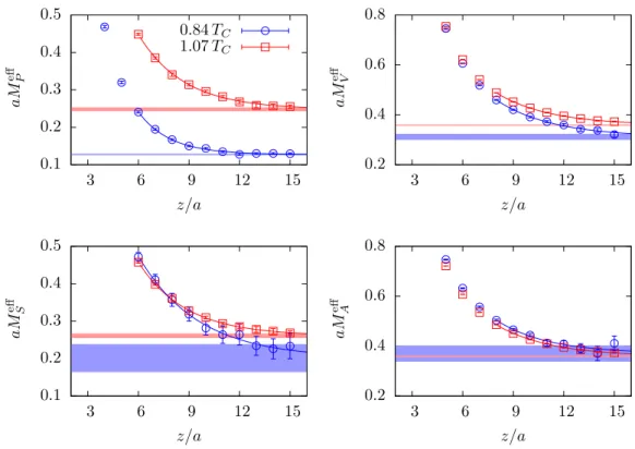
3.3 Screening masses and chiral symmetry restoration pattern

We now turn to the investigation of screening masses and the chiral symmetry restoration pattern. Since the behaviour of screening masses below and close toT_C in general depends on the quark mass we will focus on the scans along LCPs in this section, i.e. on scans C1 and D1.

The screening correlators have been measured in thex₃direction on the stored configu- rations using unsmeared point sources. To make efficient use of the generated configurations we have computed the correlation functions for 48 randomly chosen source positions (see also [64]). Compared to ref. [58], we have thus enlarged the statistics by another factor of three. Screening masses are extracted from the effective mass,² aM_X^eff, defined by the formula for the inverse hyperbolic cosine,

aM_X^eff(z) = ln



C(z+a) +C(z−a)

2C(z) +

sC(z+a) +C(z−a) 2C(z)

2

−1



 , (3.2)

where C = C_XX. Since in scans C1 and D1 the spatial extent is rather small we could not find reasonable plateaus in most of the cases due to contaminations from excited states (see also [62]). To take the contaminations into account we have fitted the results for the effective mass to the form

aM_X^eff(z) =aM_X +aAexp −∆z

, (3.3)

2Note, that the procedure differs from the one used in [62], where we have used a direct fit to the correlator. In general, the two sets of results are consistent within errors. The current set of measurements supersedes the ones from [62].