A test for stationarity based on empirical processes

SFB 823

A test for stationarity based on empirical processes

Discussion Paper

Philip Preuß, Mathias Vetter, Holger Dette

Nr. 36/2011

A test for stationarity based on empirical processes

Philip Preuß, Mathias Vetter, Holger Dette Ruhr-Universit¨at Bochum

Fakult¨at f¨ur Mathematik 44780 Bochum

Germany

email: philip.preuss@ruhr-uni-bochum.de email: mathias.vetter@ruhr-uni-bochum.de

email: holger.dette@ruhr-uni-bochum.de

September 16, 2011

Abstract

In this paper we investigate the problem of testing the assumption of stationarity in locally stationary processes. The test is based on an estimate of a Kolmogorov-Smirnov-type distance between the true time-varying spectral density and its best approximation through a stationary spectral density. Convergence of a time-varying empirical spectral process indexed by a class of certain functions is proved and furthermore the consistency of a bootstrap procedure is shown, which is used to approximate the limiting distribution of the test statistic. Compared to other methods proposed in the literature for the problem of testing for stationarity the new approach has at least two advantages. On the one hand the test can detect local alternatives converging to the null hypothesis at a rate 1/√

T (whereT denotes the sample size). On the other hand the method only requires the specification of one regularization parameter. The finite sample properties of the method are investigated by means of a simulation study and a comparison with two other tests is provided which have been proposed in the literature for testing stationarity.

AMS subject classification: 62M10, 62M15, 62G10

Keywords and phrases: spectral density, non stationary processes, goodness-of-fit tests, empirical spec- tral measure, integrated periodogram, locally stationary process, bootstrap

1 Introduction

Most literature in time series analysis assumes that the underlying process is second-order stationary.

This assumption allows for an elegant development of powerful statistical methodology like parameter estimation or forecasting techniques, but is often not justified in practice. In reality most processes change their second-order characteristics over time and numerous models have been proposed to ad- dress this feature. Out of the large literature we mention exemplarily the early work on this subject by Priestley (1965), who considered oscillating processes. More recently the concept of locally stationary processes has found considerable attention, because in contrast to other proposals it allows for a mean- ingful asymptotic theory, which is essential for statistical inference in such models. The class of locally stationary processes was introduced by Dahlhaus (1996) and particular important examples are time varying ARMA models.

While many estimation techniques for locally stationary processes were developed [see Neumann and von Sachs (1997), Dahlhaus et al. (1999), Chang and Morettin (1999), Dahlhaus and Polonik (2006), Dahlhaus and Subba Rao (2006), Van Bellegem and von Sachs (2008) or Palma and Olea (2010) among others], semiparametric testing has found much less attention although its importance was pointed out by many authors. von Sachs and Neumann (2000) proposed a method to test the assumption of station- arity, which is based on the estimation of wavelet coefficients by a localised version of the periodogram.

Paparoditis (2009) and Paparoditis (2010) used an L₂-distance between the true spectral density and its best approximation through a stationary spectral density to measure deviations from stationarity, and most recently Dwivedi and Subba Rao (2010) developed a Portmanteau-type test statistic to detect non-stationarity. However, besides the choice of a window width for the localised periodogram which is inherent in essentially any statistical inference for locally stationary processes, all these methods require the choice of at least one additional regularization parameter. It was pointed out in Sergides and Pa- paroditis (2009) that it is the choice of this particular tuning parameter that can influence the results of the statistical analysis substantially (the procedure proposed by these authors uses an additional smoothing bandwidth for the estimation of the local spectral density).

Recently Dette et al. (2011) proposed a test for stationarity which is based on anL₂-distance between the true spectral density and its best stationary approximation and which does not require the choice of that additional regularization parameter. Roughly speaking these authors proposed to estimate the L2-distance considered by Paparoditis (2009) by calculating integrals of powers of the spectral density directly via Riemann sums of the periodogram. By this idea, Dette et al. (2011) avoided the integra- tion of the smoothed periodogram [as it was done in Paparoditis (2009) or Paparoditis (2010)]. In a comprehensive simulation study it was shown that this method is superior compared to the other tests, no matter how the additional smoothing bandwidths in these procedures are chosen.

Although the test proposed by Dette et al. (2011) has attractive features it can only detect local alter- natives converging to the null hypothesis at a rateT^−1/4 (here and throughout this paperT denotes the sample size). It is the purpose of the present paper to develop a test for stationarity in locally stationary processes which can on the one hand detect alternatives converging to the null hypothesis at the rate T^−1/2 and on the other hand requires only the specification of one regularization parameter. For this

purpose we employ a Kolmogorov-Smirnov-type test statistic to estimate a measure of deviation from stationarity, which is defined by

D := sup

(v,ω)∈[0,1]²

|D(v, ω)|,

where for all (v, ω)∈[0,1]² D(v, ω) := 1

2π Z v

0

Z πω 0

f(u, λ)dλdu−v Z πω

0

Z 1 0

f(u, λ)dudλ , (1.1)

and f(u, λ) denotes the time-varying spectral density. Note that the quantity D is obviously zero if the process is stationary (i.e. f(u, λ) is does not depend on u). The consideration of functionals of the form (1.1) for the construction of a test for stationarity is very natural and was already suggested by Dahlhaus (2009). In particular, Dahlhaus and Polonik (2009) proposed an estimator of this quantity which is based on the integrated pre-periodogram (with respect to the Lebesgue measure). However, in applications Riemann sums are used to approximate the integral and therefore the approach proposed by these authors is not directly implementable. In particular, it is pointed out in Example 2.7 of Dahlhaus (2009) that the asymptotic properties of an estimator based on Riemann approximation are an open problem so far (see the discussion at the end of Section 2 for more details).

In Section 2 we introduce an alternative stochastic process, say{Dˆ_T(v, w)}(v,w)∈[0,1]², which is based on a summation of powers of the localised periodogram and serves as an estimate of {D(v, w)}(v,w)∈[0,1]². The proposed statistic does neither require integration of the localised periodogram with respect to an absolute continuous measure nor the problematic choice of a second regularization parameter. Weak convergence of a properly standardized version of ˆD_T to a Gaussian process is established under the null hypothesis, local and fixed alternatives, giving a consistent estimate ofD. The distribution of the limiting process depends on certain features of the data generating process, which are difficult estimate.

Therefore the second purpose of this paper is the development of an AR(∞) bootstrap method and a proof of its consistency (see Section 3 for details). We also provide a solution of the problem mentioned in the previous paragraph and prove weak convergence of an Riemann approximation for the integrated pre-periodogram proposed by Dahlhaus (2009) (see Theorem 2.2 in the following section). As a result we obtain two empirical processes estimating the function D defined in (1.1) which differ by the use of localised periodogram and the pre-periodogram in the Riemann approximations. In Section 4 we investigate the finite sample properties by means of a simulation study. Although the use of the pre- periodogram does not require the specification of any regularization parameter, it is demonstrated that it yields substantially less power compared to the statistic based on the localised periodogram.

Additionally, it is also shown that the latter method is extremely robust with respect to different choices of the window width, which is used for the calcualtion of the localised periodogram. Moreover we also provide a comparison with the test proposed in Dette et al. (2011) and show that their proposal is outperformed by the new method in most cases. Finally, for the sake of a transparent presentation of the results all technical details are deferred to an appendix in Section 5.

2 The test statistic

Following Dahlhaus and Polonik (2009), we define a locally stationary process via a sequence of stochas- tic processes {X_t,T}_t=1,...,T which exhibit a time-varying MA(∞) representation, namely

X_t,T =

∞

X

l=−∞

ψ_{t,T ,l}Zt−l, t= 1, . . . , T, (2.1)

where the random variables Z_t are independent identically standard normal distributed random vari- ables. Since the coefficientsψt,T ,l are in general time dependent, each process {Xt,T}t=1,...,T is typically not stationary. To ensure that the process shows approximately stationary behaviour on a small time interval, we impose that there exist twice continuously differentiable functions ψ_l : [0,1] → R (l ∈ Z) such that

∞

X

l=−∞

sup

t=1,...,T

|ψ_{t,T ,l}−ψ_l(t/T)|=O(1/T) (2.2)

asT → ∞. Furthermore, we assume that the following technical conditions

∞

X

l=−∞

sup

u∈[0,1]

|ψ_l(u)||l|<∞, (2.3)

∞

X

l=−∞

sup

u∈[0,1]

|ψ_l⁰(u)|<∞, (2.4)

∞

X

l=−∞

sup

u∈[0,1]

|ψ_l⁰⁰(u)|<∞ (2.5)

are satisfied, which are in general rather mild [see Dette et al. (2011) for more details]. Note that variablesZ_twith time varying varianceσ²(t/T) can be included in the model by choosing the coefficients ψ_{t,T ,l} in (2.1) appropriately.

Define

ψ(u,exp(−iλ)) :=

∞

X

l=−∞

ψ_l(u) exp(−iλl), then the function

f(u, λ) = 1

2π|ψ(u,exp(−iλ))|²

is well defined and called the time varying spectral density of {X_t,T}_t=1,...,T [see Dahlhaus (1996)]. It is continuous by assumption and can roughly be estimated by a local periodogram. To be precise we assume without loss of generality that the total sample size T can be decomposed as T =N M, where N and M are integers and N is even. We then define the local periodogram at time uby

I_N^X(u, λ) := 1 2πN

N−1

X

s=0

XbuTc−N/2+1+s,Texp(−iλs)

2

[see Dahlhaus (1997)], where we have set Xj,T = 0, if j 6∈ {1, . . . , T}. This is the usual periodogram computed from the observations XbuTc−N/2+1,T, . . . , X_buTc+N/2,T. It can be shown that

E(I_N^X(u, λ)) =f(u, λ) +O(1/N) +O(N/T)

and therefore the statistic I_N^X(u, λ) is an asymptotically unbiased estimator for the spectral density if N →0 andN =o(T). However, I_N^X(u, λ) is not consistent just as the usual periodogram.

We now consider an empirical version of the function D(v, ω) defined in (1.1), that is DˆT(v, ω) := 1

T

bvMc

X

j=1 bω^N₂c

X

k=1

I_N^X(uj, λk)− bvMc M

1 T

M

X

j=1 bω^N₂c

X

k=1

I_N^X(uj, λk), (2.6)

where the points

u_j := t_j

T := N(j−1) +N/2

T , j = 1, ..., M define an equidistant grid of the interval [0,1] and

λ_k := 2πk

N , k = 1, ..., N 2

denote the Fourier frequencies. It follows from the proof of Theorem 2.1 in the Appendix that for every v ∈[0,1] and ω∈[0,1] we have

E( ˆD_T(v, ω)) = 1 T

bvMc

X

j=1 bω^N

2c

X

k=1

f(u_j, λ_k)−bvMc M

1 T

M

X

j=1 bω^N

2c

X

k=1

f(u_j, λ_k) +O(1/N) +O(N²/T²)

=D(v, ω) +O(1/N) +O(N/T)

due to the approximation error of the Riemann sum. This error can be improved, if we replaceD(v, ω) by its discrete time approximation, that is

DN,M(v, ω) :=D

bvMc

M ,bω^N₂c

N 2

, for which the representation

E( ˆD_T(v, ω)) =D_N,M(v, ω) +O(1/N) +O(N²/T²) (2.7)

holds. The approximation error of the Riemann sum in (2.7) becomes smaller due to the choice of the midpointsu_j. The rate of convergence will be T^−1/2 later on, so we need the O(·)-terms to vanish asymptotically after multiplication with √

T. Therefore we define an empirical spectral process by Gˆ_T(v, ω) :=√

T1 T

bvMc

X

j=1 bω^N

2c

X

k=1

I_N^X(u_j, λ_k)− bvMc M

1 T

M

X

j=1 bω^N

2c

X

k=1

I_N^X(u_j, λ_k)−D_N,M(v, ω) ,

and assume

N → ∞, M → ∞, T^1/2

N →0, N

T^3/4 →0.

(2.8)

Our first result specifies the asymptotic properties of the empirical process ( ˆG_T(v, ω))(v,ω)∈[0,1]² both under the null hypothesis

H₀ :f(u, λ) is independent of u (2.9)

corresponding to the stationary case and the alternative. The proof is complicated and therefore deferred to the Appendix. Throughout this paper the symbol⇒ denotes weak convergence in [0,1]².

Theorem 2.1 If the assumptions (2.2)–(2.5) and (2.8) are satisfied, then as T → ∞ we have ( ˆG_T(v, ω))(v,ω)∈[0,1]² ⇒(G(v, ω))(v,ω)∈[0,1]²,

(2.10)

where (G(v, ω))(v,ω)∈[0,1]² is a Gaussian process with mean zero and covariance structure Cov(G(v₁, ω₁), G(v₂, ω₂)) = 1

2π Z 1

0

Z πmin(ω1,ω2) 0

(1_[0,v1](u)−v₁)(1_[0,v2](u)−v₂)f²(u, λ)dλdu.

Under the null hypothesis we haveD_N,M(v, ω) = 0 for allN, M ∈IN and for allv, ω ∈[0,1]. Therefore we obtain

(√

TDˆ_T(v, ω))(v,ω)∈[0,1]² ⇒(G(v, ω))(v,ω)∈[0,1]², which yields

√

T sup

(v,ω)∈[0,1]²

|Dˆ_T(v, ω)|−−→^D sup

(v,ω)∈[0,1]²

|G(v, ω)|

(2.11)

under the null hypothesis (2.9). An asymptotic level α test is then obtained by rejecting the null hypothesis of stationarity whenever √

T sup(v,ω)∈[0,1]²|Dˆ_T(v, ω)| exceeds the (1−α)% quantile of the distribution of the random variable sup(v,ω)∈[0,1]²|G(v, ω)|. The asymptotic properties under the alter- native will imply consistency of this test. Note also that under the null hypothesis H₀ the covariance structure of the limiting process in Theorem 2.1 simplifies to

(2.12) Cov(G(v₁, ω₁), G(v₂, ω₂)) = min(v₁, v₂)−v₁v₂ 2π

Z πmin(ω1,ω2) 0

f²(λ)dλ

and depends on the unknown spectral density f. In order to avoid the estimation of the integral of the squared spectral density we propose to approximate the quantiles of the limiting distribution by an AR(∞) bootstrap, which will be described in the following section.

An alternative [asymptotically unbiased, but again not consistent] estimator for the time-varying spec- tral density is given by

J_T(u, λ) := 1 2π

X

k:1≤buT+1/2±k/2c≤T

XbuT+1/2+k/2cXbuT+1/2−k/2cexp(−iλk),

which is called the pre-periodogram [see Neumann and von Sachs (1997)]. Based on this statistic we define an alternative process by

Hˆ_T¹(v, ω) :=√ T 1

T²

bvTc

X

j=1 bω^T

2c

X

k=1

J_T(j/T, λ_k,T)− bvTc T³

T

X

j=1 bω^T

2c

X

k=1

J_T(j/T, λ_k,T)−D(v, ω) , (2.13)

whereλ_k,T = ^2πk_T . The convergence of the finite dimensional distributions of the process (H_T¹(v, ω))(v,ω)∈[0,1]²

has already been shown in Dahlhaus (2009). Tightness can be shown using similar arguments as given in the Appendix for the proof of Theorem 2.1, which are not given here for the sake of brevity. As a consequence we obtain the following result.

Theorem 2.2 If the assumptions (2.2)–(2.5) and (2.8) are satisfied, then as T → ∞ we have ( ˆH_T¹(v, ω))(v,ω)∈[0,1]² ⇒(G(v, ω))(v,ω)∈[0,1]²,

where (G(v, ω))(v,ω)∈[0,1]² is the Gaussian process defined in Theorem 2.1.

Because the use of ˆH_T¹(v, ω) instead of ˆG_T(v, ω) does not require the choice of the quantity N, which specifies the number of observations used for the calculation of the local periodogram, it might be appealing to construct a Kolmogorov-Smirnov-type test for stationarity on the basis of this process.

However, we will demonstrate in Section 4 by means of a simulation study that for realistic sample sizes the method which employs the pre-periodogram is clearly outperformed by the approach based on the local periodogram. Moreover, our numerical results also show that the use of the local periodogram is not very sensitive with respect to the choice of the regularization parameterN either, and therefore we strictly recommend to use the latter approach when constructing a Kolmogorov-Smirnov test.

Remark 2.3 The convergence of a modified version of the process (2.13) to the limiting Gaussian pro- cess (G(v, ω)(v,ω))∈[0,1]² of Theorem 2.1 was shown in Dahlhaus and Polonik (2009), where the Riemann sum over the Fourier frequencies was replaced by the integral with respect to the Lebesgue measure.

More precisely, these authors considered the process ( ˆH_T²(v, ω))(v,ω)∈[0,1]² := 1

2π√ T

bvTc

X

j=1

Z πω 0

JT(j/T, λ)dλ−v

T

X

j=1

Z πω 0

JT(j/T, λ)dλ−D(v, ω)

(v,ω)∈[0,1]²

instead of (H_T¹(v, ω))(v,ω)∈[0,1]² and proved its weak convergence. Note also that asymptotic tightness has neither been studied for an integrated nor for a summarized local periodogram in the literature so far. Moreover, many other asymptotic results are only shown for the integral of the local periodogram or pre-periodogram instead of the sum over the Fourier coefficients [see for example Dahlhaus (1997) or Paparoditis (2010)]. The transition from these results to analogue statements for the corresponding Riemann approximations is by no means obvious. For example, although it is appealing to assume that

Z π 0

I_N^X(u, λ)dλ= 2π N

N 2

X

k=1

I_N^X(u, λ_k) +O(1/N)

because of the Riemann approximation error, this fact is in general not true, as the derivative ^∂INX_∂λ^(u,λ) is not uniformly bounded in N [a demonstrative explanation of this fact is that I_N^X(u, λ_k1) andI_N^X(u, λ_k2) are asymptotically independent whenever k₁ 6= k₂]. Thus in general asymptotic results for the inte- grated local periodogram or pre-periodogram can not be directly transferred to corresponding Riemann approxiamtions. These difficulties were also explicitly pointed out in Example 2.7 of Dahlhaus (2009).

Remark 2.4 A careful inspection of the proofs in the Appendix shows that (2.10) also holds in the case where

(2.14) f(u, λ) =f(λ) +g_Tk(u, λ)

if g_T = o(1/√

T). Here k is an appropriate function such that (2.14) defines a time-varying spectral density. Moreover, if gT = ^√1

T, an analogue of Theorem 2.1 can be obtained where the centering term D_N,M(v, ω) in the definition of ˆG_T(v, ω) is replaced by

D_N,M,k(v, ω) = 1 2π√

T

Z ^bvM_M^c

0

Z

2πbω N 2c N

0

k(u, λ)dλdu− bvMc M

Z

2πbω N 2c N

0

Z 1 0

k(u, λ)dudλ (note that f(u, λ) is replaced by ^√1

Tk(u, λ) in the definition of D_N,M). In this case the appropriately centered process converges weakly to a Gaussian process {G(v, ω)}_{(v,ω)∈[0,1]}² with covariance structure given by (2.12). A similar comment applies to the process ˆH_T¹ defined in (2.13). This means that the tests based on the processes ˆG_T and ˆH_T¹ can detect alternatives converging to the null hypothesis at a rate T^−1/2. In contrast, the proposal of Dette et al. (2011) is based on an L₂-distance between f(u, λ) andR1

0 f(v, λ)dv and is therefore only able to detect alternatives converging to the null hypothesis at a rate T^−1/4.

3 Bootstrapping the test statistic

To approximate the limiting distribution of sup(v,ω)∈[0,1]²|G(v, ω)|, we employ an AR(∞)-bootstrap approximation, which was introduced by Kreiß (1988). The bootstrap works by fitting anAR(p)-model

(p∈IN) to the data X1,T, ..., XT ,T, where the parameterp=p(T) increases with the sample size T. To be precise we first calculate an estimator (ˆa_1,p, ...,aˆ_p,p) for

(a_1,p, ..., a_p,p) = argmin

b1,p,...,bp,p

E X_t,T −

p

X

j=1

b_j,pX_t−j,T2

(3.1)

and then simulate a pseudo-series X_1,T^∗ , ..., X_T,T^∗ according to the model X_t,T^∗ =X_t,T; t= 1, ..., p,

X_t,T^∗ =

p

X

j=1

ˆ

a_j,pX_t−j,T^∗ +Z_j^∗; p < t≤T.

Here the quantitiesZ_j^∗ denote normal distributed random variables with mean zero and variance ˆ

σ²_p := 1 T −p

T

X

t=p+1

(ˆz_t−z_T)², (3.2)

wherez_T := _T¹_−pPT

t=p+1zˆ_t and ˆ

z_t :=X_t,T −

p

X

j=1

ˆ

a_j,pXt−j,T for t=p+ 1, ..., T

[in other words ˆσ²_p is the standard variance estimator of the error process ˆz_t]. We now define the statistic Gˆ^∗_T(v, ω) in the same way as ˆG_T(v, ω) where the original observations X_1,T, ..., X_T,T are replaced by the bootstrap replicatesX_1,T^∗ , ..., X_{T ,T}^∗ . To assure that this procedure approximates the limiting distribution corresponding to the null hypothesis both under the null hypothesis and the alternative, we define the stationary processX_t^AR(p) as the process which is defined through

X_t^AR(p) =

p

X

j=1

a_j,pX_t−j^AR(p) +Z_t^AR(p),

whereZ_t^AR(p) is a Gaussian white noise process with mean zero and variance σ²_p =E X_t−

p

X

j=1

a_j,pXt−j

!2

,

whereX_tdenotes the stationary process with spectral densityR1

0 f(u, λ)du. We now impose the following technical conditions:

Assumption 3.1

(i) p=p(T)∈[p_min(T), p_max(T)], where p_max(T)≥p_min(T)−−−−→ ∞^T→∞ and p³_max(T)p

log(T)

√T =O(1) (3.3)

(ii) The stationary process Xt with strictly positive spectral density R1

0 f(u, λ)du has an AR(∞)- representation, i.e.

X_t=

∞

X

j=1

a_jXt−j +Z_t^AR (3.4)

where (Z_j^AR)_j∈Z denotes a Gaussian white noise process with variance σ² >0, P∞

j=1|a_j|<∞ and 1−

∞

X

j=1

a_jz^j 6= 0 for |z| ≤1.

(iii) The estimators for the AR parameters defined by (3.1) satisfy

1≤j≤pmax|ˆa_j,p−a_j,p|=O(p

log(T)/T) (3.5)

uniformly with respect to p≤p(T).

(iv) The estimate σˆ_p² defined in (3.2) converges in probability to σ² >0 .

All assumptions are rather standard in the framework of an AR(∞)-bootstrap [see for example Kreiß (1997) or Berg et al. (2010)] and it follows from Lemma 2.3 in Kreiß et al. (2011) that there exists a p₀ ∈IN such that for allp≥p₀ theAR(p)-process defined through (3.1) has anM A(∞)-representation

X_t^AR(p) =

∞

X

l=0

ψ^AR_l (p)Z_t−l^AR(p).

(3.6)

Furthermore assumption (3.5) and Lemma 2.3 in Kreiß et al. (2011) imply that there exist a p⁰₀ ∈IN, such that for all p≥p⁰₀ the fitted AR(p)-process has an M A(∞)-representation

X_t,T^∗ =

∞

X

l=0

ψˆ^AR_l (p)Z_t−l^∗ .

Because of (2.8) and (3.3), assumption (3.5) is for example satisfied for the least squares or the Yule- Walker estimators [see Hannan and Kavalieris (1986)]. These estimates have also the desired property that the fitted AR(p)-process has an M A(∞)-representation for every p, if at least two observations are different which is typically the case. Note that (2.3) together with Lemma 2.1 of Kreiß et al. (2011) imply

∞

X

j=1

j|a_j|<∞, (3.7)

which will be used in the proof of the following theorem.

Theorem 3.2 If the assumptions (2.2)–(2.5), (2.8) and Assumption 3.1 are satisfied, then as T → ∞ we have conditionally on X_1,T, ..., X_{T ,T}

( ˆG^∗_T(v, ω))(v,ω)∈[0,1]² ⇒( ˜G(v, ω))v∈[0,1],ω∈[0,1],

where ( ˜G(v, ω))(v,ω)∈[0,1]² denotes a centered Gaussian process with covariance structure Cov( ˜G(v₁, ω₁),G(v˜ ₂, ω₂)) = min(v₁, v₂)−v₁v₂

2π

Z πmin(ω1,ω2) 0

Z 1 0

f(u, λ)du2

dλ.

We now obtain empirical quantiles of sup(v,ω)∈[0,1]²|G(v, ω)|by calculating ˆD_T,i^∗ := sup(v,ω)∈[0,1]²|Gˆ^∗_{T ,i}(v, ω)|

fori= 1, ..., Bwhere ˆG^∗_T,1(v, ω), ...,Gˆ^∗_{T ,B}(v, ω) are theBbootstrap replicates of ˆG_T(v, ω). We then reject the null hypothesis, whenever

√

T sup

(v,ω)∈[0,1]²

|Dˆ_T(v, ω)|>( ˆD_T^∗)T ,b(1−α)Bc, (3.8)

where ( ˆD_T^∗)_T,1, ...,( ˆD^∗_T)_{T ,B} denotes the order statistic of ˆD_{T ,1}^∗ , ...,Dˆ_{T ,B}^∗ . This test has asymptotic levelα because of Theorem 3.2 and is consistent, since conditionally on X_1,T, ..., X_{T ,T} each bootstrap statistic sup(v,ω)∈[0,1]²|Gˆ^∗_T(v, ω)| converges to a non generate random variable, while √

T sup(v,ω)∈[0,1]²|Dˆ_T(v, ω)|

converges to infinity by Theorem 2.1. We finally point out that similar results can be shown for the statistic which is obtained by replacing in ˆDT the localised periodogram by the pre-periodogram. The technical details are omitted for the sake of brevity, but the finite sample performance of this alternative approach will be investigated in the following section.

4 Finite sample properties

4.1 Choosing the parameter

We first comment on how to choose the parameters N and p in concrete applications. Although the proposed method does not show much sensitivity with respect to different choices of both parameters, we select p throughout this section as the minimizer of the AIC criterion [see Akaike (1973)], which is defined by

ˆ

p= argmin_p1 T

T 2

X

k=1

log(fθ(p)ˆ (λ_k,T) + I_T^X(λ_k,T) fθ(p)ˆ (λ_k,T)

+p/T

in the context of stationary processes [see Whittle (1951) or Whittle (1952)]. Herefθ(p)ˆ is the spectral density of a stationary AR(p) process with the fitted coefficients and I_T^X is the usual stationary peri- odogram. Therefore we focus in the following discussion on the sensitivity analysis of the test (3.8) with respect to different choices of the parameter N. In particular it will be demonstrated in several examples that the test is very robust with respect to different choices of N.

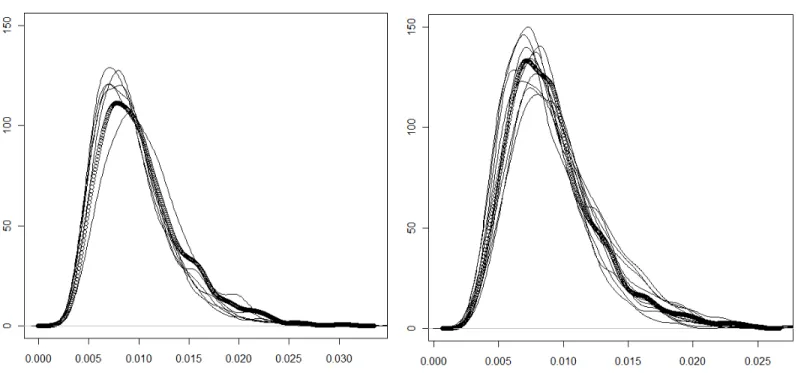
Figure 1: Estimated densities of the distribution of the statistic √

T sup(v,ω)∈[0,1]²|Dˆ_T(v, ω)| under the null hypothesis. The dotted line is the estimated exact density while the solid lines corresponds to the estimated densities of the bootstrap approximations. Left panel: N = 8; right panel: N = 16.

4.2 Bootstrap approximation

We now illustrate how the proposed bootstrap method approximates the distribution of the statistic

√Tsup(v,ω)∈[0,1]²|Dˆ_T(v, ω)| under the null hypothesis. For this purpose we generated observations of the stationaryAR(1) model

X_t,T = 0.5X_t−1,T +Z_t t= 1, ..., T forT = 128 and calculated the bootstrap test statistic√

T sup(v,ω)∈[0,1]²|Dˆ_T(v, ω)|both for N = 16 and N = 8. For both cases we generate 1000 replicates to estimate the exact distribution and chose randomly 10 series from the 1000 replications for which we calculate 1000 bootstrap approximations. Based on the 1000 bootstrap replications we estimate the density of the corresponding bootstrap approximation.

The plots are given in Figure 1 where the dotted line corresponds to the estimated exact density while the dashed lines show the 10 estimated densities of the bootstrap approximations.

4.3 Size and power of the test

In this section we investigate the size and power of the test (3.8) and the analogue based on the pre-periodogram. We also compare these methods with a test, which has recently been proposed by Dette et al. (2011). All reported results are based on 200 bootstrap replications and 1000 simulation

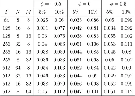
φ =−0.5 φ= 0 φ= 0.5

T N M 5% 10% 5% 10% 5% 10%

64 8 8 0.025 0.06 0.035 0.086 0.05 0.099 128 16 8 0.031 0.077 0.042 0.081 0.034 0.092 128 8 16 0.03 0.076 0.038 0.083 0.055 0.102 256 32 8 0.04 0.086 0.051 0.106 0.053 0.111 256 16 16 0.038 0.089 0.044 0.085 0.045 0.08 256 8 32 0.036 0.083 0.051 0.098 0.05 0.102 512 64 8 0.054 0.103 0.052 0.084 0.042 0.09 512 32 16 0.046 0.083 0.044 0.09 0.049 0.092 512 16 32 0.038 0.079 0.056 0.098 0.052 0.099 512 8 64 0.05 0.102 0.047 0.101 0.051 0.112

Table 1: Rejection probabilities of the test (3.8) under the null hypothesis. The data was generated according to model (4.1).

runs under the null hypothesis while we used 500 simulation runs under the alternative. To study the approximation of the nominal level we simulate AR(1) processes

X_t=φX_t−1+Z_t, t∈Z (4.1)

and M A(1) processes

X_t=Z_t+θZt−1, t∈Z (4.2)

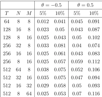
for different values of the parameters φ and θ. The corresponding results are depicted in Table 1 and 2 and we observe a precise approximation of the nominal level for φ ∈ {−0.5,0,0.5} and θ = 0.5 even for very small samples sizes. Furthermore, if T gets larger, the results are basically not affected by the choice of N in these cases. For θ = −0.5 the nominal level is underestimated for smaller T but for T = 512 the approximation of the nominal level becomes much more precise and is robust with respect to different choices of the window widthN if it is chosen according to the assumptions (2.8) (so basicallyN should be larger than M).

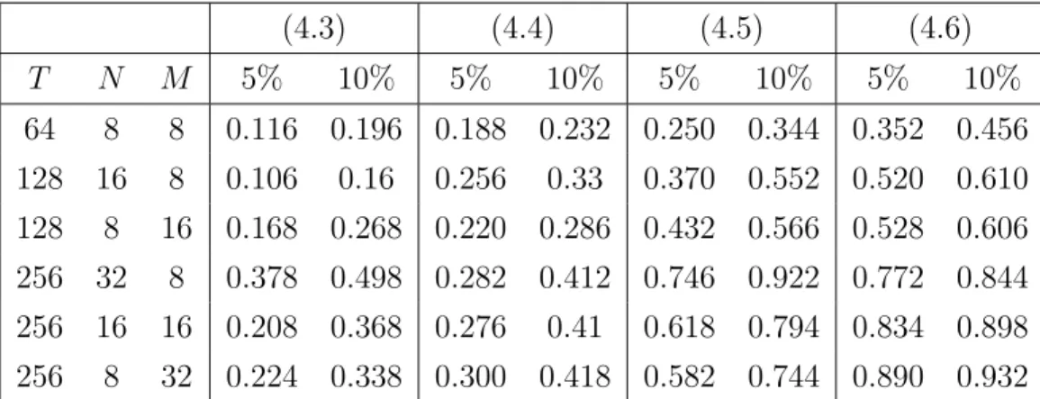
To study the power of the test (3.8) we simulated data from the following four models which corresponds

θ =−0.5 θ= 0.5

T N M 5% 10% 5% 10%

64 8 8 0.012 0.041 0.045 0.091 128 16 8 0.023 0.05 0.043 0.087 128 8 16 0.025 0.043 0.05 0.102 256 32 8 0.033 0.081 0.04 0.074 256 16 16 0.025 0.061 0.043 0.083 256 8 16 0.025 0.057 0.059 0.112 512 64 8 0.038 0.075 0.052 0.106 512 32 16 0.035 0.075 0.047 0.094 512 16 32 0.029 0.058 0.05 0.093 512 8 64 0.025 0.053 0.07 0.116

Table 2: Rejection probabilities of the test (3.8) under the null hypothesis. The data was generated according to model (4.2).

to the alternative of a non-stationary process Xt,T = (1 +t/T)Zt

(4.3)

X_t,T =−0.9 rt

TXt−1,T +Z_t (4.4)

X_t,T =

(0.5X_t−1+Z_t if 1≤t≤ ^T₂,

−0.5Xt−1+Z_t if ^T₂ + 1≤t ≤T. (4.5)

Xt,T =







0.5Xt−1+Z_t if 1≤t≤ ^T₂,

10Zt if ^T₂ + 1≤t≤ ^T₂ +₆₄^T , 0.5Xt−1+Z_t if ^T₂ +₆₄^T + 1 ≤t≤T. (4.6)

The corresponding rejection probabilities are reported in Table 3 and we observe a reasonable behavior of the procedure in all considered cases. Under the alternative the bootstrap test (3.8) is also robust with respect to different choices of N. Note that even for the choice M = 32, N = 8, which clearly contradicts (2.8), the results are satisfying.

It might be of interest to compare these results with other tests for the hypothesis of stationarity which have been suggested in the literature. Because we are interested in procedures, which require as less as possible regularization we restrict ourselves to a comparison with two procedures. In Table 5 we present the rejection frequencies if we use the pre-periodogram [which was defined in (2.13)] instead of the local periodogram in our approach [see Theorem 2.2 and the discussion at the end of Section 2]. Recall that the use of the pre-periodogram does not require the specification of the value N, which specifies the