Tests based on sign depth for multiple regression

SFB 823

Tests based on sign depth for multiple regression

Discussion Paper

Nr. 7/2020

Melanie Horn · Christine H. M¨uller

Abstract The extension of simplicial depth to robust regression, the so-called simplicial regression depth, provides an outlier robust test for the parameter vector of regression models. Since simplicial regression depth often reduces to counting the subsets with alternating signs of the residuals, this led recently to the notion of sign depth and sign depth test. Thereby sign depth tests generalize the classical sign tests.

Since sign depth depends on the order of the residuals, one generally assumes that theD-dimensional regressors (explanatory variables) can be ordered with respect to an inherent order. While the one- dimensional real space possesses such a natural order, one cannot order these regressors that easily for D >1 because there exists no canonical order of the data in most cases.

For this scenario, we present orderings according to the Shortest Hamiltonian Path and an approxima- tion of it. We compare them with more naive approaches like taking the order in the data set or ordering on the basis of a single quantity of the regressor. The comparison bases on the computational runtime, stability of the order when transforming the data, as well as on the power of the resulting sign depth tests for testing the parameter vector of different multiple regression models. Moreover, we compare the power of our new tests with the power of the classical sign test and theF-test. Thereby, the sign depth tests based on our distance based approaches show similar power as theF-test for normally distributed residuals with the additional benefit of being much more robust against outliers.

Keywords Sign test·data depth·multiple regression·Shortest Hamiltonian Path·Traveling Salesman Problem·nearest neighbor method

Melanie Horn (Corresponding Author) Faculty of Statistics, TU Dortmund University Tel.: +49-231-7553114

E-mail: mhorn@statistik.tu-dortmund.de Christine H. M¨uller

Faculty of Statistics, TU Dortmund University Tel.: +49-231-7554238

E-mail: cmueller@statistik.tu-dortmund.de

1 Introduction

In many regression models, only a single outlier can distort the parameters of the model. When testing these parameters, often the parameters of the true model get rejected if only one outlier exists in the data set. A well-known example is the F-test in least-square regression. The literature provides many robust estimators and some robust tests for parameters of regression models, see e.g. the books of Rieder (1994), Jureˇckov´a and Sen (1996), M¨uller (1997), Rousseeuw and Leroy (2003), Huber (2004), Jureˇckov´a and Picek (2005), Maronna et al. (2006), Hampel et al. (2011), Clarke (2018). Most of the developed robust regression methods have the disadvantage that a tuning parameter must be chosen. This is not the case for an approach based on data depth introduced by Rousseeuw and Hubert (1999) extending the half space depth of Tukey (1975) to regression depth.

The half space depth has many extensions. Most of them concern multivariate data; see, for example simplicial depth of Liu (1990), zonoid depth treated in Mosler (2002), Mahalanobis depth as used in Hu et al. (2011) or functional data as in L´opez-Pintado and Romo (2009), Claeskens et al. (2014), Agostinelli (2018). Not all of them provide robust methods and most of them concern only estimation.

There are not many extensions of the half space depth to regression and in particular to robust testing. M¨uller (2005) showed that simplicial regression depth, an extension of Liu’s simplicial depth to the regression depth of Rousseeuw and Hubert (1999), can be used for testing the parameters of a regression model robustly. Kustosz et al. (2016b) proved that the simplicial regression depth often reduces to counting the subsets with alternating signs of the residuals so that Leckey et al. (2019) defined K- sign depth via the relative number of subsets of K observations with alternating signs of the residuals.

This leads toK-sign depth tests which generalizes the classical sign test and can be used as soon as the residuals are independent with median zero under the null hypothesis.

The asymptotic distribution of the 3-sign depth was derived in Kustosz et al. (2016a) for AR(1)- regression, however the proof holds for any 3-sign depth if the residuals are independent with median equal to zero. For small sample sizes and not too largeK, the distribution of the K-sign depth can be easily simulated. Using such distributions, Kustosz et al. (2016a), Kustosz et al. (2016b), and Leckey et al.

(2019) show for several examples that 3-sign depth tests and 4-sign depth tests are much more powerful than the classical sign test and reach the power of the classical nonrobust tests based on least squares of the residuals. However these examples are restricted to the case where the regressor (explanatory variable) is one dimensional so that there is a natural ordering of residuals. Thereby, the ordering is crucial for determining the relative number of subsets of alternating signs of residuals.

Therefore, it is not clear how to extend this approach for the case of multivariate regressors. We propose two types of distance based ordering of the regressors, namely a method based on the Shortest Hamiltonian Path and an approximation of it. These distance based methods have also the advantage that they can be used for ordinal regressors as soon as a distance measure is given. We compare these approaches with more naive methods like using the order of the data set, random order or ordering based on projections or norms of the regressors.

This paper is organized as follows: In Section 2, the sign depth and the corresponding sign depth tests are defined. Section 3 presents the used approaches for ordering multidimensional regressors and compares these approaches by the computational runtime and stability of the order when transforming the data. In Section 4, a simulation study is presented which compares the different approaches of Section 3 with respect to the power of the resultingK-sign depth tests for testing the parameter vector of different multiple regression models. In this section, also the power of these approaches are compared with the power obtained by the classical sign test and theF-test. A conclusion and outlook is given in Section 5.

2 Test Based on Sign Depth in the Context of Regression

In this paper, we focus on multiple linear regression. Hence, at first the notation of a linear regression model is introduced, before the sign depth and the corresponding test is introduced.

2.1 Notation for Multiple Linear Regression

Lety= (y₁, . . . , y_N)^>∈R^N,e= (e₁, . . . , e_N)^>∈R^N,θ,x_n ∈R^D, andX= (x₁, ...,x_N)^>∈R^N×Dwith N, D∈N. Then, a multiple linear regression model is given by

y=Xθ+e.

Here, the errors e₁, . . . , e_N are realizations of stochastically independent random variables E₁, . . . , E_N with P(E_n<0) =P(E_n >0) = 0.5. The latter assumption in particular says that the probability of an error to be zero is zero. These assumptions hold for example for every error distribution which is continuous and has a median equal to zero, like the standardized normal distribution or the standardized Cauchy distribution. With the definition ofz_n:= (y_n,x^>_n)^>∈R^D+1andZ:= (z₁, ...,z_N)^>, the residual relating toz_n and a parameter vectorθ is given byres(z_n,θ) :=y_n−x^>_nθ.

2.2 The Sign Depth

As Rousseeuw and Hubert (1999) noticed for simple linear regression and Kustosz et al. (2016b) proved in the context of linear and nonlinear regression and autoregression, the simplicial regression depth often reduces to what we call the K-sign depth. Hence, the K-sign depth, with K ≥ 2, can be seen as a generalization of the simplicial regression depth introduced by M¨uller (2005) for generalized linear models. We define theK-sign depth as follows:

Definition 1 Let x1, ...,xN be ordered according to some criteria andK ∈Nwith 2≤K < N. Then theK-sign depth d^K_S of parameterθin the data setZ is defined via:

s⁽¹⁾_n

k :=

K

Y

k=1

1{res(znk,θ)·(−1)^k >0}

s⁽²⁾_n

k :=

K

Y

k=1

1{res(zn_k,θ)·(−1)^k <0}

d^K_S(θ,Z) :=

N K

−1

X

1≤n1<n₂<···<nK≤N

(s⁽¹⁾_n

k +s⁽²⁾_n

k)

where 1{...} denotes the indicator function, which is one if the condition in the curly braces holds and zero otherwise.

●

●

●

●

0

●

●

●

●

●

●

alternating signs ●

0

●

●

●

●

●

●

●

alternating signs

0

●

●

●

●

●

●

●

no alternating signs

0

●

●

●

●

●

●

●

no alternating signs

0

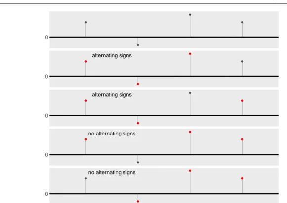
Fig. 1Example of calculating the K-sign depth with parameter K= 3. The topmost figure shows four residuals of an arbitrary model, the lower figures show the ⁴₃

= 4 combinations of 3-tuples of these residuals. Here, two out of four 3-tuples have alternating signs, so the 3-sign depth is 0.5

In short, the K-sign depth is the relative number of ordered K-tuples with alternating signs of the residuals. It can be used as soon as a given ordering of the residuals is available. An example of calculating the 3-sign depth can be found in Figure 1.

Note that the value of the K-sign depth depends on the ordering of the regressors. In simple linear regression with only one explanatory variable (and possibly an intercept), there exists a distinct order of the regressors according to the values of the explanatory variable. But for regression with more than one explanatory variable, one can think of many different criteria for ordering the regressors. Our aim for this paper is to propose some possible ordering criteria and compare them with regard to theoretical properties, like stability of the order when transforming the data, and practical behavior in a simulation study. An example why the ordering criterion has a crucial effect on the sign depth is given in Example 1 below.

Example 1 Lety =Xθ+e be a linear regression model withxn = (1, xn1, xn2)^>, xn1, xn2∈ [−1,1], θ = (θ0, θ1, θ2)^> and En i.i.d.N(0,0.01). The true model has the parameter vectorθtrue = (0,1,1)^>. N = 16 observations of this model are given. To these data points, a regression model with the parameter vector ˆθ = (−0.05,−0.5,1)^> is fitted. A visualization of the data points and the fitted model can be found below in Figure 2. It can be seen that the fitted model produces eight positive residuals and eight negative residuals.

Fig. 2 Visualization of the 16 data points (red) and the fitted model (dark grey)

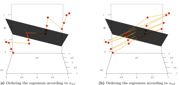
A possible method for ordering the regressors is to sort the regressors according to the values of only one explanatory variable and neglect the values of all other (see Section 3.2.) In this example, this would lead to two possible orders which are shown below in Figure 3.

(a)Ordering the regressors according toxn1 (b)Ordering the regressors according toxn2

Fig. 3 Visualization of two possible orders for the 16 regressors. The order is marked as orange line

As discussed below, these two orders lead to very different values of theK-sign depth. When ordering according to the values of xn1, only one sign change in the residuals occurs. Ordering according to the values ofxn2leads to seven sign changes. This has crucial effect on all theK-sign depths withK≥3, as it can be seen in Table 1.

Table 1 K-sign depth withK∈ {2, 3,4,5} for the orders (a) and (b) of Figure 3

d²_S(ˆθ,Z) d³_S(ˆθ,Z) d⁴_S(ˆθ,Z) d⁵_S(ˆθ,Z)

(a) 0.533 0 0 0

(b) 0.533 0.286 0.176 0.088

In this paper, we will focus on the case K= 3 andK= 4 because the 3-sign depth and 4-sign depth are equivalent with the simplicial regression depth for a regression model with a parameter vector θ which is two-dimensional and three-dimensional, respectively (Kustosz et al., 2016b). For a small number of observations (up to approximately N = 25), the distributions can be calculated exactly. For this, the 3-sign depth and the 4-sign depth of all 2^N possible sign combinations of the residuals have to be calculated. For a larger number of observations, simulation of the distributions is possible by using not all possible sign combinations but only a random subset. When the number of observations is sufficiently large, an asymptotic distribution of the standardized 3-sign depth N·(d³_S(θ,Z)−0.25) was shown in (Kustosz et al., 2016a). The derivation of the asymptotic distribution of the general K-sign depth is in progress. This work indicates thatK-sign depth can be calculated in linear time using an asymptotically equivalent form which is exact for 3-sign depth and 4-sign depth.

2.3 The Sign Depth Test

On the basis of theK-sign depth, testing the parameters of a regression model can be done. When the fitted parameter vector of a model is correct, the residuals scatter independently of each other around zero. In contrast, if the fitted parameter vector is not correct, the independence of the signs of the residuals is often violated and the residuals do not scatter around zero. This leads to fewerK-tuples with alternating signs and hence to a smaller K-sign depth. When the value of theK-sign depth is smaller than theα-quantile of the distribution of the correspondingK-sign depth, it is shown significantly to the levelα∈(0,1) that the considered model does not fit the data. TheK-sign depth test can be written as follows:

Theorem 1 K-Sign Depth Test

Let α∈ (0,1) and K ∈N be fixed with 2 ≤K < N, whereN is the number of observations in the dataset Z. Let q_α^K,N denote the α-quantile of the distribution of the K-sign depth for N observations.

Then, the test

ϕ^K(θ,Z) =1

sup

θ∈Θ0

d^K_S(θ,Z)< q_α^K,N

is a test to the level αforH0:θ∈Θ0 vs.H1:θ∈/Θ0.

Hence, the K-sign depth test rejects the null hypothesis H0 : θ ∈ Θ0 if the K-sign depth of all parametersθ of the null hypothesis setΘ0 is too small. For a proof of this simple test strategy based on data depth, see M¨uller (2005).

The K-sign depth test is a generalization of the classical sign test since the 2-sign depth test is equivalent with the classical sign test, see Leckey et al. (2019). For testingH0:θ=θ0 vs.H1:θ6=θ0, the classical sign test is given by

ϕ(θ,Z) =1{N+∈/ [bN,0.5,α/2, bN,0.5,1−α/2]},

whereN+ ≤N is the number of positive residuals andb_N,0.5,α/2andbN,0.5,1−α/2denote theα/2-quantile and (1−α/2)-quantile of the binomial distribution with parametersN and 0.5.

3 Methods for Ordering Multidimensional Data

As Example 1 shows, the order of the regressors is of high importance for the value of the sign depth and the result of the sign depth test. In the next subsections some possible criteria for ordering the regressors are presented, where not only the ordering methods are studied, but also their computational runtime and their behavior when transforming the data.

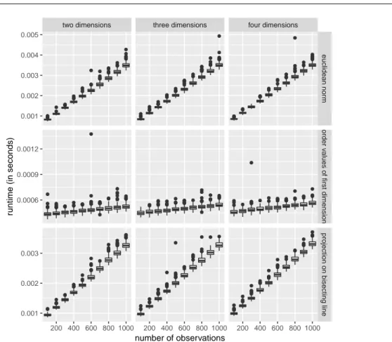
All computational results in this section and Section 4 were obtained with the software R (R Core Team, 2018) and our self-writtenR-packageGSignTest(Horn, 2019), in which all presented methods of this paper are implemented, including the ordering methods, theK-sign depth, theK-sign depth tests, the classical sign test and theF-test for regression models. The package is freely available on Github. The graphics in this paper were created using the packagesggplot2 (Wickham, 2009),gridExtra(Auguie, 2017) and rgl(Adler et al., 2018). The simulations were performed on the High Performance Cluster LiDO3¹ of the TU Dortmund University.

In this section, we use computational results to demonstrate the differences between the methods for ordering multidimensional data. To show the main concepts of the ordering methods, we use two data sets where each contains 20 two-dimensional regressors in [−1,1]². The first data set, called LHS, is obtained by a Latin Hypercube Sampling (LHS) with maximizing the minimal distance between two points (Stein, 1987). The regressors of the second one, called Spiral, are arranged as a spiral with little noise. To compare the runtimes of the methods, we simulated 200 times a data set with 100×k, k= 1, . . . ,10, two-, three- and four-dimensional regressors using uniformly distributed random values in [−1,1] for every dimension of the regressors.

3.1 Naive Methods

The simplest methods for ordering multidimensional data are taking the order the observations appear in the data set or taking a random order. These two methods are equivalent if the order of the observations in the data set is already a random order. Because the order does not depend on the observations itself but on the index of the observation, these two methods are stable when applying transformation on the data, which may be important in some situations.

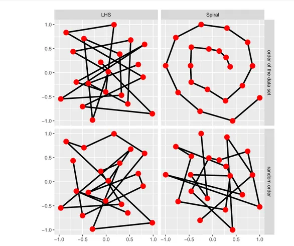
Figure 4 shows the obtained order by these methods with the help of the LHS and Spiral data sets.

It can be seen that the two methods are equivalent for the LHS data because the used R-package lhs (Carnell, 2019) provides the regressors already in a random order. On the other hand, the two methods differ very much on the Spiral data set because the used R-packagemlbench (Leisch and Dimitriadou, 2010) provides the regressors in a natural order.

1 https://lido.tu-dortmund.de/cms/de/LiDO3/index.html

●

●

●

●

●

●

●

●

●

● ●

●

●

●

●

●

●

●

●

●

●

●

●

●

●

●

●

● ●

●

●

● ●

● ●

●

●

●

●

●

●

●●

● ●

●

●

●

●

●

●

●

● ●

●

●

●

●

●

●

●

●

● ●

●

●

●

●

●

●

●

●

●

● ●

●

●

●

●

●

LHS Spiral

order of the data setrandom order

−1.0 −0.5 0.0 0.5 1.0 −1.0 −0.5 0.0 0.5 1.0

−1.0

−0.5 0.0 0.5 1.0

−1.0

−0.5 0.0 0.5 1.0

Fig. 4 Example of the two naive ordering methods described in Section 3.1: according to the data set (upper row) and random ordering (lower row). The left figures provide regressors of a two-dimensional Latin Hypercube Sampling (LHS) and the right figure’s regressors are arranged as a two-dimensional spiral

Another advantage of these two methods is the runtime of the ordering process. When no ordering is done, the runtime obviously is O(1). When a random order is used, the Fisher-Yates-algorithm for randomly permuting data, which is used inR, has a runtime ofO(N) (Durstenfeld, 1964). This behavior can also be seen in Figure 5. There, the empirical runtimes of sorting different regressor and dimension numbers are shown. As the theoretical runtimes say, the runtime of both methods does not depend on the number of dimensions. In addition, it can be seen that the runtimes are very small, so that only little time in the whole testing process has to be spent on the ordering process here.

●●

●

●●

●

●

●●

●

●●

●●

● ●●●

● ●●● ●

●

●●

●● ●●●● ●●●●●● ●●●●

●●

●●

●●

● ●●

●

●

●

●●

●

●● ●●●●●●● ●● ●●●● ●●●●

● ●●

●

●●

●●

●● ●●●

●●

●●

●

●

●●

●●

●

●●

●●

● ●●●●●●●

●●

● ●●●●●●●● ●●●●●●●●

●

●● ●● ●●●● ●●●●●

●

●●

●

● ●●●●● ●●● ●●●

● ●●

● ●●● ●●●●● ●●●●● ●●●●

●●

● ●●

●

●●

●●

●●

●●

●●

●●

●

●

●

●● ●●●●

● ●●●●●● ●●●

●

●●

●●

●● ●●●●●

●

●

●●

●●

●●

●●

●

●●

●

●

●●

● ●●●●●●

●

●

● ●●

●

●

●●

●●

●

●●

●●

● ●●●●●● ●●●●

● ●●●● ●●●● ●●●●

●●

●●

● ●

●●

●●

two dimensions three dimensions four dimensions

order of the data setrandom order

200 400 600 800 1000 200 400 600 800 1000 200 400 600 800 1000 0.0002

0.0004 0.0006 0.0008 0.0010

0.0002 0.0004 0.0006 0.0008 0.0010

number of observations

runtime (in seconds)

Fig. 5 Empirical runtimes of the two naive ordering methods described in Section 3.1: according to the data set (upper row) and random ordering (lower row)

3.2 Scalarization Based Methods

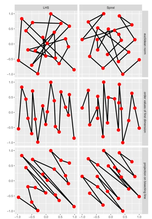
Another approach for ordering multidimensional data is ordering the regressors on the basis of scalarized values of each regressor. One possible scalarization is taking an arbitrary vector norm. Another method is projecting all regressors orthogonal on a line, for example the bisecting line. A special case of the orthogonal projection is ordering the regressors on the basis of the values of only one dimension, like in Example 1. Here, the regressors are projected on a line parallel to a coordinate axis. A disadvantage of all scalarizations is that the order directly depends on the values of the regressors. When transforming the data, the order might get completely different which is unwanted in most cases. An example of this behavior can be found in Example 1: When flipping the coordinate axes (or changing the projection the ordering is based on), the sign depth test can come to completely contrary results. When taking the norm as the scalarization, the ordering highly depends on the origin of the coordinate system because every vector norm produces positive values, no matter if the values in the vector are positive or negative. Figure 6 shows an example of the ordering on the same two data sets like in Section 3.1.

Besides the disadvantage of the non-stable order by data transformation, an advantage of the scalariza- tion based methods is the rather short runtime for computing the order. Many scalarization methods, like calculating an arbitrary vector norm as well as projecting the regressor on an arbitrary line, need linear runtime. Because a single regressor has dimensionD∈N, the runtime for computing the scalarized value of one regressor isO(D). Doing this for allN∈Nregressors, this leads to a runtime of O(N D). Sorting these values can be done in approximately O(N), when usingRadix Sort (Knuth, 1998), which is used inRby default for 200 up to 100 000 numeric values. Overall, the runtime for ordering multidimensional regressors according to a scalarized value scales linearly in the number of regressors and dimensions, i.e.

O(N D). The special case of the projection method, using only the values of one dimension for ordering,

●

●

●

●

●

●

●

●

●

●

●

● ●

●

●

●

●

●

●

●

●

●

●

●

●

●

●

●

●

●

●

●

●

●

●

●

●

●

●

●

●

●

●

● ●

●

●

●

●

●

●

●

●

●

●

●

●

●

● ●

●

●

●●

●

●

●

●

●

●

●

●

●

●

●

●

●

●

●

●

●

●

●

●

●

●

●

●

●

● ●

●

●

●

●

●

●

●

●

●

●

●

●

●

●

●

●

●

●

●

●

●

●

●

●●

●

●

●

●

LHS Spiral

euclidean normorder values of first dimensionprojection on bisecting line

−1.0 −0.5 0.0 0.5 1.0 −1.0 −0.5 0.0 0.5 1.0

−1.0

−0.5 0.0 0.5 1.0

−1.0

−0.5 0.0 0.5 1.0

−1.0

−0.5 0.0 0.5 1.0

Fig. 6Example of three scalarization based ordering methods described in Section 3.2: ordering according to the euclidean norm (upper row), according to the projection on the first dimension (middle row), and according to the projection on the bisecting line (lower row)

●

●

●●

●●

●

●

●

●

●

●

●

●●

●●

●

●●

●●

●

●

●

●●

●●

●

●

●●

●

●●

●●

●

●●

●●

●

●

●●

●●

●

●●

●

●

●

●●

●●

●●

● ●●●●● ●●●● ●●●● ●●

●

●●

●

●

●

●●

●●

●

●

●●

●

●

●

●●

● ●

●●

●

●

●

●●

●●

●

●

●

●●

●●

●

●●

●

●●

●

●●

●

●

●●

●

●

● ●

●●

●

●●

●●

●

●●

●●

●●

●

●

●●

●●

●

●●

●●

●

●●

●● ●●●

●●

●

●

●

●●

●●

●●

●

●

●●

●●

●●

●●

●●

●

●

●

●●

●● ●●●●●

●

●

●

●

●

●●

● ●

●●

●● ●

●

●●

●● ●●

●

● ●●●●●● ●

●

●

●

●

●●

●

● ●●

● ●●

●●

●●

●

●●

●●

●●

●●

●●

●

●●

●

●

●●

●●

●●

●●

●

●

●●

●●

●

●●

●●

●

●

●

●

● ●

●

●●

●

●

●●

●

●

●

●

●●

●●

●●

●

●

●

●●

● ●●●●●

●

●●

●

●●

●●

●

●

●●

● ● ●●●●●

●

● ●● ●●●●● ●●●●●●● ●●

●

●●

● ●●● ●●

●

●

●●

●●

●

●●

●

●

●●

●

●

●

●

●●

●●

●

●

●●

●● ●

●

●

●●

●

●●

●

●

●●

●

●

●

●●

●●

●

●

●●

●

●●

●●

two dimensions three dimensions four dimensions

euclidean normorder values of first dimensionprojection on bisecting line

200 400 600 800 1000 200 400 600 800 1000 200 400 600 800 1000 0.001

0.002 0.003 0.004 0.005

0.0006 0.0009 0.0012

0.001 0.002 0.003

number of observations

runtime (in seconds)

Fig. 7 Empirical runtimes of the three scalarization based ordering methods described in Section 3.2:

ordering according to the euclidean norm (upper row), according to the projection on the first dimension (middle row), and according to the projection on the bisecting line (lower row)

can be sped up by using directly the radix sort algorithm on the values of the considered dimension. This leads to an approximative linear runtime which is independent of the number of dimensions, i.e. O(N).

When looking at Figure 7 with the empirical runtimes of both methods including the special case, it can be seen, that all scalarization based methods seem to scale linearly in the number of regressors. In contrast, the linear trend in the number of dimensions is neglectable. On the other hand, it can be seen that using only the values of one dimension for sorting is much faster than its generalization. But overall, the runtimes of these ordering methods are very small.

3.3 Distance Based Methods

Taking the values of the regressors for ordering has some disadvantages as explained in Section 3.2. For this, an alternative can be to compute an order based on the pairwise distances of the regressors. Then,

●

●

● ●

● ●

●

●

●

●

●

●

● ●

●

●

●

●

●

●

● ●

●

●

●

●

●

● ●

●

●

●

●

● ●

● ●

●

●

●

●

●

●

●

●

●

● ● ●

●

●

●

●

●

●

● ●

●

●

●

●

●

●

●

●

●

●

●

●

● ● ●

●

●

●

●

●

●

● ●

LHS Spiral

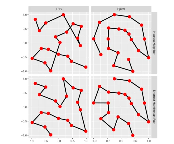
Nearest NeighborShortest Hamiltonian Path

−1.0 −0.5 0.0 0.5 1.0 −1.0 −0.5 0.0 0.5 1.0

−1.0

−0.5 0.0 0.5 1.0

−1.0

−0.5 0.0 0.5 1.0

Fig. 8Example of the two distance based ordering methods described in Section 3.3: the approximative nearest neighbor algorithm (upper row) and the exact solution of the SHP (lower row)

the ordering does not get influenced by any data transformation that does not change the relation of the distances, like flipping coordinate axes or shifting the origin of the coordinate system. Another advantage of distance based methods is that these methods can also be used for ordinal data, if the distance between two ordinal values can be expressed by a numeric value.

Ordering based on the pairwise distances of the regressors means that regressors that have a small distance to each other get ordered near to each other and regressors that have large distance are far away from each other in the ordering. Here, the term distance can mean an arbitrary distance measure, although in this paper always the euclidean distance is used. This aim for ordering can be rewritten as the problem to find a shortest path through the data. This so called Shortest Hamiltonian Path (SHP) is a simple transformation of the well-knownTraveling Salesman Problem (TSP) (Lawler et al., 1985).

Here, a solution for a complete graph has to be computed. Because the TSP (and also the SHP) belong to the so called NP-hard problems (which means in the worst case the exact solution cannot be computed in polynomial runtime), many approximative algorithms with faster runtime exist. One approximative algorithm is anearest neighbor approach. The idea is to start at an arbitrary point and always proceed