Search for massive particles decaying into multiple quarks with the ATLAS detector in √

A TLAS-CONF-2013-091 28 August 2013

ATLAS NOTE

ATLAS-CONF-2013-091

August 26, 2013

Search for massive particles decaying into multiple quarks with the ATLAS detector in √

s = 8 TeV pp collisions

The ATLAS Collaboration

Abstract

A search is conducted for hadronic decays of new massive particles in √

s = 8 TeV pp collisions using an integrated luminosity of 20.3 fb

collected by the ATLAS detector at the LHC. Gluino production in the context of supersymmetry models in which R-parity is not conserved is used as a benchmark scenario, both for the case where the gluino is the lightest supersymmetric partner, and for the case where it decays to a neutralino which then undergoes an R-parity violating decay. A selection on the number of jets, their trans- verse momenta, and the number of jets identified as originating from a b-quark is applied and a counting experiment is performed. Results are presented for all possible R-parity vi- olating branching fractions of gluino decays to various quark flavours. In a model where pair-produced gluinos each decay into three light-flavour quarks, exclusions of m

< 853 GeV (expected) and m

< 917 GeV (observed) are placed at the 95% confidence level.

Alternately, for a model where each gluino decays into one b-jet and two light quarks, ex- clusions of m

< 921 GeV (expected) and m

< 929 GeV (observed) are set. Limits are also set for decay modes to a variety of other flavours as well as for decay modes through an intermediary neutralino, which leads to 10-quark final states.

⃝ c Copyright 2013 CERN for the benefit of the ATLAS Collaboration.

Reproduction of this article or parts of it is allowed as specified in the CC-BY-3.0 license.

1 Introduction

The analysis presented here is designed as a search for new physics in various final states with a large number of high transverse momentum ( p

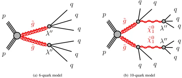
) jets. Results are interpreted in the context of two R-parity violating (RPV) supersymmetric models. In one model, which is referred to as the “6-quark model”, gluinos are pair-produced and decay promptly via a virtual (mass of 5 TeV) squark in the cascade decay ( ˜ g → qq ˜ → qqq ). In the second model, referred to as the “10-quark model”, gluinos are pair-produced and decay via an intermediate on-shell neutralino in the process ( ˜ g → q q ˜ → qq χ ˜

→ qqqqq). The diagrams corresponding to these processes are shown in Fig. 1. This is the first ever search for the 10- quark signature. Exclusion limits in the 6-quark model have been placed by the CDF collaboration with m

< 144 GeV [1], the CMS collaboration with m

< 460 GeV using 5 fb

of √

s = 7 TeV data [2], and the ATLAS collaboration with m

< 666 GeV using 4.6 fb

of data at √

s = 7 TeV [3].

This analysis updates the ATLAS RPV multi-jet search of Ref. [3] to the full 2012 √

s = 8 TeV dataset. In addition, two new results are added. Firstly, the 10-quark model is included. Secondly, b-tagging information is used to make new interpretations in the space of RPV coupling parameters.

For this analysis the Minimal Supersymmetric Standard Model (MSSM) of SUSY with R-Parity con- servation [4–17] is used but with an additional component added to the Lagrangian that allows RPV interactions. The extra terms of the Lagrangian correspond to the additional superpotential [18, 19]

W

= 1

2 λ

L

L

E ¯

+ λ

L

Q

D ¯

+ 1

2 λ

U ¯

D ¯

D ¯

+ κ

L

H

, (1) where i, j , k = 1, 2, 3 are generation indices. The subject of this analysis is the third term of this equation,

1

2

λ

U ¯

D ¯

D ¯

. It is this term that allows the gluino to decay into three quark jets in the 6-quark model. In the 10-quark model, on the other hand, it is the second decay, ˜ χ

→ qqq that proceeds via this term. The RPV Lagrangian term ensures that each decay under this coupling produces exactly one up-type quark and two down type quarks (of di ff erent flavours). The flavours of the decay products depend entirely on the values of the λ

factors, which can only be constrained by the data as they are not predicted by the model.

It is assumed that the λ

terms lead to short enough lifetimes for the ˜ g and for the ˜ χ

that the dis- placements of the RPV decays from the primary vertex are negligible, and it is further assumed that the gluino width is small compared to the detector resolution. These assumptions are in common with pre- vious RPV multijet analyses. Unlike previous RPV multi-jet analyses, flavour information is used here.

The limits that have been previously set were based upon the assumption of a 100% decay branching fraction of gluinos into three quarks and assumed that the processes would be identical for each flavour.

Some RPV terms in Eq. 1, however, lead to top quarks in the RPV decay products, which were assumed to not be present in previous searches. Other RPV terms lead to charm and bottom quarks. Dedicated selections which use b-tagging information are employed to target signatures with top, bottom and charm quarks, allowing conclusions to be drawn for various flavour RPV decays (as driven by the λ

factors).

Limits are set based upon the branching fractions of RPV decays into each given quark flavour. This analysis searches for an excess of multi-jet events by counting the number of high transverse momentum (at least 80 GeV) 6-jet and 7-jet events, with various b-tagging requirements added to enhance the sen- sitivity to couplings that favour decays to third generation quarks. The number of jets, the p

cut that is used to select jets, and the number of b-tags are optimised separately for each signal model taking into account experimental and theoretical uncertainties.

The outline of this document is as follows. Section 2 describes the ATLAS detector and the technical

reconstruction of collision events at ATLAS. Section 3 describes the data samples used in the analy-

sis. Section 4 discusses the background determination, and provides a number of data-driven studies to

validate and estimate uncertainties on the background models. Section 5 discusses the systematic un-

(a) 6-quark model (b) 10-quark model

Figure 1: Feynman diagrams for the gluino decays used as benchmarks for this search. Diagrams for (a) the 6-quark model and (b) the 10-quark model are shown.

Section 6.

2 Detector, data acquisition, and object definitions

The ATLAS detector [20, 21] provides nearly full solid angle coverage around the collision point with an inner tracking system covering |η| < 2.5

, electromagnetic and hadronic calorimeters covering |η| < 4.9, and a muon spectrometer covering |η| < 2 . 7.

The ATLAS tracking system is comprised of a silicon pixel tracker closest to the beamline, a mi- crostrip silicon tracker, and a straw-tube transition radiation tracker at radii up to 108 cm. These systems are layered radially around each other in the central region. A thin solenoid surrounding the tracker provides an axial 2 T field enabling measurement of charged particle momenta. The track reconstruction efficiency ranges from 78% at p

= 500 MeV to more than 85% above 10 GeV, with a transverse impact parameter resolution of 10 µ m for high momentum particles in the central region. The overall acceptance of the inner detector (ID) spans the full range in ϕ , and the pseudorapidity range |η| < 2 . 5 for particles originating near the nominal LHC interaction region.

The calorimeter comprises multiple subdetectors with several di ff erent designs, spanning the pseu- dorapidity range up to |η| = 4 . 9. The measurements presented here use data from the central calorimeters that consist of the Liquid Argon (LAr) barrel electromagnetic calorimeter (|η| < 1.475) and the Tile hadronic calorimeter (|η| < 1.7), as well as two additional calorimeter subsystems that are located in the forward regions of the detector: the LAr electromagnetic end-cap calorimeters (1 . 375 < |η| < 3 . 2), and the LAr hadronic end-cap calorimeter (1.5 < |η| < 3.2). As described below, jets are required to have

|η| < 2.8 such that they are fully contained within the barrel and end-cap calorimeter systems.

The jets used for this analysis are found and reconstructed using the anti-k

algorithm [22, 23] with a radius parameter R = 0 . 4. The energy of the jet is corrected for inhomogeneities and for the non- compensating nature of the calorimeter by weighting the energy deposits in the electromagnetic and the hadronic calorimeters separately by factors derived from the simulation and validated with the data [24].

1

The ATLAS reference system is a Cartesian right-handed coordinate system, with the nominal collision point at the origin.

The anticlockwise beam direction defines the positive

point to the centre of the LHC ring and the positive

is measured around the beam

axis, and the polar angle

is measured with respect to the

ln[tan(

)], rapidity is defined

as

0

5 ln[(E

)

(E p

)], where

is the energy and

is the

defined as

sin

The jets are further corrected to remove the energy deposits from secondary collisions in the event and from the collisions of other partons within the same protons [25]. In some signal regions either one or two jets are also required to be identified as originating from b-quarks (“b-tagged”). b-tagging at ATLAS uses multivariate algorithms that identify b-hadrons based upon the displacement of individual tracks and upon the displacement, mass, and fragmentation properties of any secondary vertices that are reconstructed within the jet [26]. For this search a tagger was used with an operating setting at a tagging efficiency of roughly 70% for real b-jets in t t ¯ events. Due to the limited geometrical acceptance of the ID, b-tagging is only considered for jets with |η| < 2 . 5.

Trigger decisions at ATLAS are made in three stages: Level 1, Level 2, and the Event Filter. The Level-1 trigger is implemented in hardware and uses a subset of detector information to reduce the event rate to a design value of at most 75 kHz. This is followed by two software-based triggers, Level-2 and the Event Filter, which together reduce the event rate to a few hundred Hz. The measurement presented in this note uses multi-jet triggers which, for the analysis selections used, are more than 99% efficient. The multi-jet triggers implemented at the Event Filter Level have access to the full detector granularity, which allows selection of multi-jet events with high e ffi ciency. Di ff erent triggers are used depending on whether the event will be included in a signal region of the analysis or a control region. The trigger for events that are selected for the signal regions requires six jets with at least 45 GeV of transverse momentum.

When selecting events in data with fewer than six jets for background studies, prescaled triggers were chosen. These prescales were compensated for by weighting events based upon the prescale setting that was active at the time of the collision. For all signal regions in this analysis, however, the jets have a high enough p

for each trigger to be fully e ffi cient.

The data used in this analysis represents 20.3 ± 0.6 fb

of integrated luminosity, corresponding to the entire 2012 ATLAS data-taking period [27]. All collision events are required to have met baseline data quality criteria.

3 Simulated events

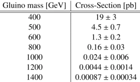
Simulated samples of pair-produced gluinos are used to estimate the expected signal yield. Several signal models consisting of various mass spectra and decay topologies are considered. The gluino pair- production cross-sections are determined at next-to-leading order in the strong coupling constant, adding the resummation of soft gluon emission at next-to-leading-logarithmic accuracy (NLO + NLL) [28–32].

The total cross-sections and uncertainties for each gluino mass that is considered in this analysis are summarized in Table 1.

Gluino mass [GeV] Cross-Section [pb]

400 19 ± 3

500 4 . 5 ± 0 . 7

600 1.3 ± 0.2

800 0 . 16 ± 0 . 03 1000 0 . 024 ± 0 . 006

1200 0.0044 ± 0.0014

1400 0 . 00087 ± 0 . 00034

Table 1: The signal cross-sections for pp → g˜ ˜ g production depending on gluino mass. The cross- sections are determined with associated theoretical uncertainties at NLO with next-to-leading-logarithm soft gluon resummation (NLO + NLL) (see Section 5.2 for more details).

For gluino pair simulations of the 6-quark and 10-quark models, Herwig++ 6.520 [33] interfaced

showering, hadronization, and underlying event. For the 10-quark model, each produced gluino is forced to decay to two quarks and a neutralino through standard R-parity conserving (RPC) couplings. The neutralinos then undergo the λ

decay to three quarks. The neutralino is considered the lightest su- persymmetric particle here and is, therefore, considered to be on-shell. Samples are produced covering the m

vs m

1

space with gluino mass points of 400, 600, 800, 1000, 1200, and 1400 GeV. For each gluino mass, separate samples are generated with neutralino masses of 50, 300, and 600 GeV where the latter is only produced for gluino masses of at least 1 TeV. For each point in m

vs m

1

space, 30000 events are generated using H erwig++ . For the 6-quark gluino model events are produced for each of the following mass points: 500, 600, 800, 1000, and 1200 GeV. In the generation of the samples, all possible λ

flavour decay modes are allowed to proceed with equal probability. Results for models with alternate decay modes (resulting from models with alternate λ

values) are determined by weighting events based upon the flavor of their simulated decay modes. All samples are produced assuming that the gluino width is narrow.

The largest background for this analysis is from multi-jet production. This contribution is estimated from the data aided by dijet events simulated with P ythia 6.426 [35] where two partons are produced in a hard-scatter and a multi-jet final state is produced with a parton shower model. This simulation is discussed in more detail when describing its use in Section 4.2. Other backgrounds are small, however after b-tagging they are not negligible. The second largest background is from t¯ t production in the fully hadronic decay channel. These events are modeled using MC@NLO 4.06 [36] interfaced to Herwig 6.520 [37] with underlying event modeled using Jimmy [38]. Other significant background processes are t¯ t pairs that decay into one or more leptons, which is modeled using S herpa 1.4.1 [39], and W + jets, which is modeled using the Alpgen 2.14 generator [40] interfaced to Pythia 6.426.

These events are processed in a simulation [41] of the detector using G eant 4 [42]. The e ff ect of multiple pp interactions is taken into account in the simulation, though due to the high-p

requirements that are placed on the jets, it does not impact the analysis significantly.

4 Background Predictions

4.1 Introduction to the background estimation

The background yield in each signal region is estimated by starting with a signal-depleted control region in data and projecting it into the signal region using a factor that is determined from a multi-jet simulation, with corrections applied to account for additional minor background processes. Rather than treating systematic uncertainties on the background estimation separately, as commonly done, such uncertainties are not divided into categories such as jet energy uncertainties, showering uncertainties, etc. Instead, a single systematic uncertainty on the background yield is determined by comparing the background prediction to the data in a wide variety of control regions. The spread in predictions from many control regions defines the total background uncertainty in the signal region.

4.2 Simulated samples for the background projection

For the multi-jet simulation that is used to make projections from background control regions into the

signal region, one challenge is that a large number of events are required at both very high jet p

and

multiplicity (for the signal regions) and at low jet p

and low multiplicity (for the control regions). Fur-

ther, one of the requirements of the data-driven error estimation procedure (discussed in Sections 4.4

and 4.5) is that the simulated projection factors must evolve in a consistent way between low and high

jet multiplicity regions. Generators such as Pythia are well-suited to these requirements as they can gen-

erate events very quickly (allowing the production of su ffi ciently large datasets) and have no transition

in behaviour with growing parton multiplicities. This is not the case for multileg matrix elements gen- erators when considering parton multiplicities above that of the hard interaction and jets from the parton shower enter the selection. Such a transition between models of jet production has the potential to cause discontinuities in the multijet spectra important to this analysis. The ATLAS tune AUET2B LO** [43]

of P ythia 6.426 was observed to reproduce the data well in the 7 TeV analysis, and was therefore chosen again for this 8 TeV analysis.

The P ythia multi-jet background events are generated in separate samples filtered by leading jet p

in order to ensure that enough events are available in all relevant kinematic ranges, using roughly 45 million events. Since it is slow to simulate the detector e ff ects, these samples are used at particle level and a Gaussian smearing is applied in order to account for jet energy resolution effects [44]. These jets are constructed from interacting final state particles using the same anti-k

algorithm with a radius parameter of R = 0 . 4 as is used for o ffl ine jets. Muons, neutrinos, and pileup particles are not included in the clustering. Similarly, differences in jet merging or splitting between particle jets and jets reconstructed in the detector are not modeled. The e ff ect of particle-level mismodeling is found to be non negligible but is covered by the total systematic uncertainties evaluated using the data-driven techniques described in Section 5. The b-tagging efficiencies are applied to each simulated jet as a function of the jet flavour,

p

, and η as determined in dedicated b-tagging calibration measurements [45–48].

4.3 Background projections

The background normalizations are determined by projecting to the signal regions from control regions using projection factors that are derived from the simulation and validated in the data. Validations of these projections are shown in a wide variety of control regions that are used to determine systematic uncertainties on the background estimation in later sections. The formula used for the projections is:

N

= (

N

− N

)

×

 

 N

N

 

 + N

(2)

In this equation, the number of background events with n jets (N

) is determined starting from the number of events in the data with m jets (N

). The projection factor,

n−jetMC

N_m^MC_−jet

, is determined from the multi-jet simulation. Other minor corrections from other backgrounds (“OtherBGs”: t t, single top, ¯ and W + jet events) are also applied based upon estimates from the simulation. Without b-tagging, the contribution of events from OtherBGs is around 1%. Including two b-tags increases this contribution to roughly 10%.

When the projection is performed with n chosen to be five or less, the background is much larger

than the expected signal contribution. Such projections are used to validate the background model for the

purpose of assigning systematic uncertainties. When n is larger than five the expected signal contribution

can become significant for some models. These selection requirements are considered as candidate

signal regions. An optimization is performed to choose the actual signal region used for a given model

and is discussed in Section 6.1. Although other choices are also studied to determine background yield

systematic uncertainties from the data, the backgrounds in the final signal regions are evaluated using

projections across two jet multiplicity bins (n = m + 2). This choice was verified to lead to small signal

contamination in the control regions.

4.4 Background projection validation and systematic uncertainties from lower jet mul- tiplicity data

Since the 3, 4, and 5-jet multiplicity bins have minimal expected signal contamination they are useful for validating the background model. The basic validation of the background prediction is performed by projecting the background from the m = 3 or m = 4 jets into the n = 5 jets control region and comparing with the data. This comparison is shown in Fig. 2, which shows the number of events passing a given jet p

cut with a 5 jet requirement. It is seen that the projection has a good accuracy in the extrapolations to the 5-jet bin in data, both with and without the requirement of b-tagging. The conclusion of this validation study is that Eq. 2 can be used with no correction factors, but a systematic uncertainty on the method should be applied to account for the discrepancies between data and the prediction in the validation regions. This systematic is required to cover the largest discrepancy that is observed between data and the prediction when projecting from either the 3-jet or 4-jet bins into the 5-jet control region, as well as from projections to higher jet multiplicity to be discussed shortly.

4.5 Background validation cross-checks and systematic uncertainties

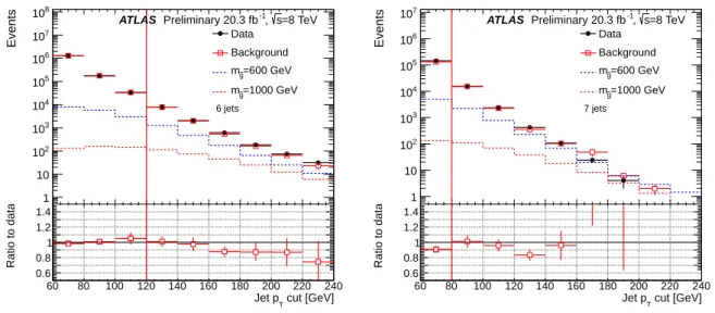
In Section 4.4 it was shown that the projection factor is accurate when projecting into the five jet bin from lower jet multiplicity bins. It is important to also verify that such projection factors are still correct at higher jet multiplicities. As a first cross-check a projection is performed into the six and seven exclusive jet bins but with a low enough jet p

requirement to serve as a background control region. Any jet mul- tiplicity bins with a signal contribution of more than 10% for the 600 GeV 6-quark model were not used as control regions, and were excluded from the evaluation of the background systematic uncertainties.

Results of these projections are shown in Fig. 3.

For the signal region, selection requirements are made on jet p

, jet multiplicity, and number of b-tags. Several other variables were considered, however the tight p

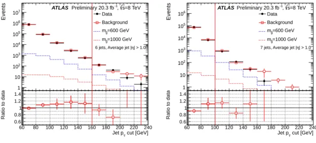
and multiplicity requirements in the signal region strongly a ff ect the event kinematics making the gains from additional kinematic re- quirements small enough that the benefits do not justify the added complexity. With looser selection requirements, however, additional kinematic variables can be used to reduce the signal contribution fur- ther and create background-enriched control regions. Among the many kinematic distributions that have been considered, one that appears to show both good discrimination between signal and Standard Model- dominated data samples, and which is well modeled by the simulation, is the average |η| of the selected jets. These kinematic shapes are shown for two di ff erent sets of selection requirements in Fig. 4. The jets from these centrally produced pairs of gluinos typically have lower values in this distribution than the uncorrelated production of jets in the background. A requirement of average jet |η| > 1 . 0 is applied to deplete the expected signal contamination for certain background studies. This choice was determined to be the tightest cut that can reasonably be performed without unacceptably depleting the sample statis- tics. Under this requirement, bins at higher jet p

had a low enough expected signal contamination to be considered for the evaluation of the systematic uncertainty. Results of these projections are shown for the 6-jet and 7-jet bins in Fig. 5. The largest deviations from the expected values were found to be a few percent larger than they were for the 5-jet projections.

For a given jet p

and tagging requirement, the final systematic uncertainties on the background are

chosen to cover the worst observed discrepancies of all projections considered so far. Specifically, the

uncertainties must be larger than the largest systematic bias observed in Fig. 2. Additionally, if any of the

projections into the lower jet p

control regions of Figs. 3 or 5 that could be observed leads to a larger

discrepancy, the background systematic uncertainty is increased to cover this difference.

60 80 100 120 140 160 180 200 220 240

Events / 20 GeV

103

104

105

106

107

108

109

1010

=8 TeV, 20.3 fb-1 s

Data

Projection from 3 Jets Projection from 4 Jets

= 600 GeV g~ m

= 1000 GeV g~ m ATLAS Preliminary

0 b-tags

≥ 5 jets,

Cut [GeV]

Jet pT

60 80 100 120 140 160 180 200 220 240

Ratio To Data

0.6 0.8 1 1.2 1.4

(a)

0

60 80 100 120 140 160 180 200 220 240

Events / 20 GeV

102

103

104

105

106

107

108

109 _-1

=8 TeV, 20.3 fb s

Data

Projection from 3 Jets Projection from 4 Jets

= 600 GeV g~ m

= 1000 GeV g~ m ATLAS Preliminary

1 b-tags

≥ 5 jets,

Cut [GeV]

Jet pT

60 80 100 120 140 160 180 200 220 240

Ratio To Data

0.6 0.8 1 1.2 1.4

(b)

1

60 80 100 120 140 160 180 200 220 240

Events / 20 GeV

10 102

103

104

105

106

107

108 Data s=8 TeV, 20.3 fb^-1

Projection from 3 Jets Projection from 4 Jets

= 600 GeV g~ m

= 1000 GeV g~ m ATLAS Preliminary

2 b-tags

≥ 5 jets,

Cut [GeV]

Jet pT

60 80 100 120 140 160 180 200 220 240

Ratio To Data

0.20.4 0.60.81 1.21.4 1.61.8

(c)

2

Figure 2: The number of observed events in the 5-jet bin is compared to the background expectation that is determined by using P ythia to project the number events in data from the low-jet multiplicity control regions. The contents of the bins represent the number of events with 5-jets passing a given jet p

cut.

These bins are inclusive in jet p

. Results with various b-tag requirements are shown.

60 80 100 120 140 160 180 200 220 240

Events

1 10 102

103

104

105

106

107

108

Data Background

=600 GeV

g~

m

=1000 GeV

g~

m 6 jets

ATLAS Preliminary 20.3 fb^-1, s=8 TeV

cut [GeV]

Jet pT

60 80 100 120 140 160 180 200 220 240

Ratio to data

0.6 0.8 1 1.2 1.4

(a) Projection from the 4-jet to the 6-jet bin

60 80 100 120 140 160 180 200 220 240

Events

1 10 102

103

104

105

106

107

Data Background

=600 GeV

g~

m

=1000 GeV

g~

m 7 jets

ATLAS Preliminary 20.3 fb^-1, s=8 TeV

cut [GeV]

Jet pT

60 80 100 120 140 160 180 200 220 240

Ratio to data

0.6 0.8 1 1.2 1.4

(b) Projection from the 5-jet to the 7-jet bin

Figure 3: The data are compared with the expected background shapes in the exclusive six and seven jet bins before b-tagging. The contents of the bins represent the number of events with the given number of jets passing a given jet p

requirement. The bins with less than 10% signal contamination are control regions that are considered when assigning systematic uncertainties on the background yield. These control regions are the bins to the left of the vertical red lines in the plots.

η| Average jet |

0 0.5 1 1.5 2 2.5

Normalized Distributions

0 0.05 0.1 0.15 0.2

0.25 ATLASPreliminary, 20.3 fb^-1, s = 8 TeV Data

=600 GeV

~g

m

=1000 GeV

~g

m

160 GeV

T≥ 3 jets, p

(a) Average jet

160 GeV

η| Average jet |

0 0.5 1 1.5 2 2.5

Normalized Distributions

0 0.05 0.1 0.15 0.2 0.25

0.3 ATLASPreliminary, 20.3 fb^-1, s = 8 TeV Data

=600 GeV

g~

m

=1000 GeV

g~

m

160 GeV

T≥ 5 jets, p

(b) Average jet

160 GeV

Figure 4: Normalized distributions of average jet |η| of the jets above the given p

threshold are shown

for the Standard Model-dominated data sample and for two signal models before b-tagging.

60 80 100 120 140 160 180 200 220 240

Events

1 10 102

103

104

105

106

107 Data

Background

=600 GeV

g~

m

=1000 GeV

g~

m

| > 1.0 η 6 jets, Average jet | ATLAS Preliminary 20.3 fb^-1, s=8 TeV

cut [GeV]

Jet pT

60 80 100 120 140 160 180 200 220 240

Ratio to data

0.6 0.8 1 1.2 1.4

(a) Projection from the 4-jet to the 6-jet bin. Average

1.0.

60 80 100 120 140 160 180 200 220 240

Events

1 10 102

103

104

105

106 Data

Background

=600 GeV

g~

m

=1000 GeV

g~

m

| > 1.0 η 7 jets, Average jet | ATLASPreliminary 20.3 fb^-1, s=8 TeV

cut [GeV]

Jet pT

60 80 100 120 140 160 180 200 220 240

Ratio to data

0.6 0.8 1 1.2 1.4

(b) Projection from the 5-jet to the 7-jet bin. Average

1.0.

Figure 5: The data are compared with the expected background shapes in the exclusive six and seven jet bins before b-tagging, and with an additional requirement of the average jet pseudorapidity |η| > 1.

The bins with less than 10% signal contamination are control regions that are considered when assigning systematic uncertainties on the background yield. These control regions are the bins to the left of the vertical red lines in the plots.

4.6 Data in the candidate signal regions

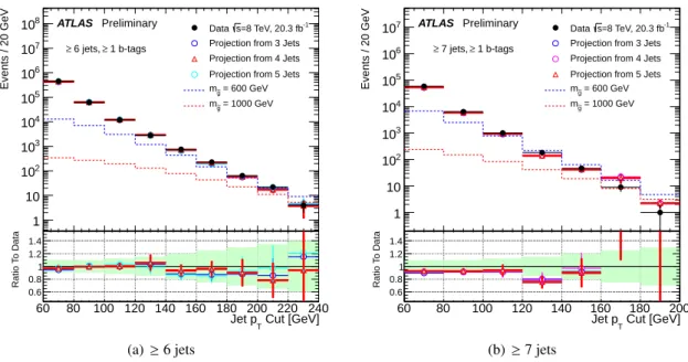
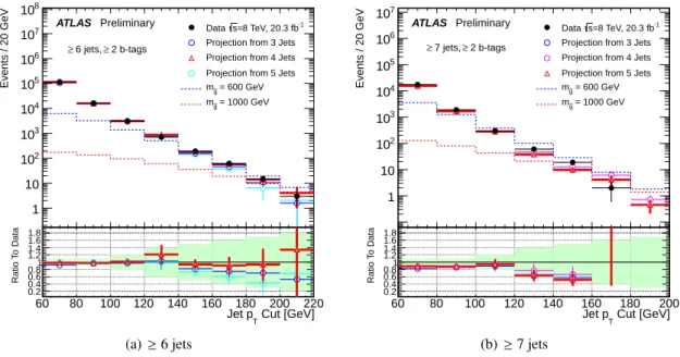
Distributions for data in the ≥ 6- and ≥ 7-jet bins are shown in Fig. 6, compared with background predictions that are determined when projecting from three different jet multiplicity bins. In each case the red distribution represents the actual background prediction that will be considered in this analysis while the other projections are simply considered as additional validation. Similarly, results after b-tagging are shown in Figs. 7 and 8. The background systematic uncertainties that were determined from the validations in data are shown as the green band in the bottom of each plot. The bins in these distributions represent candidate signal regions, which may be chosen as a real signal region for a particular model under the optimization procedure that is described in Section 6.1 except for regions deemed insensitive to the model and used as a control region in the systematic uncertainty determination. In practice it is seen that for most signals, the seven jet bin is preferred as a signal region. The data in each distribution show good agreement with background predictions within uncertainties.

5 Systematic Uncertainties

Systematic uncertainties on the background estimation are determined directly from the data as part of the background validation discussed in Section 4.5 and further discussed in Section 5.1. In contrast, sys- tematic uncertainties on the signal predictions are drawn from several sources of modeling uncertainties.

The largest systematic uncertainties are those on the background yield and the jet energy scale uncer-

tainties on the signal yield. These and all other significant uncertainties are explained in the following

sections.

60 80 100 120 140 160 180 200 220 240

Events / 20 GeV

10 102

103

104

105

106

107

108

109

=8 TeV, 20.3 fb-1

s Data

Projection from 3 Jets Projection from 4 Jets Projection from 5 Jets

= 600 GeV

g~

m

= 1000 GeV

g~

m ATLAS Preliminary

0 b-tags

≥ 6 jets,

≥

Cut [GeV]

Jet pT

60 80 100 120 140 160 180 200 220 240

Ratio To Data

0.60.7 0.8 0.91.11 1.2 1.31.4

(a)

6 jets

60 80 100 120 140 160 180 200 220

Events / 20 GeV

1 10 102

103

104

105

106

107

108

=8 TeV, 20.3 fb-1

s Data

Projection from 3 Jets Projection from 4 Jets Projection from 5 Jets

= 600 GeV

g~

m

= 1000 GeV

g~

m ATLAS Preliminary

0 b-tags

≥ 7 jets,

≥

Cut [GeV]

Jet pT

60 80 100 120 140 160 180 200 220

Ratio To Data

0.60.7 0.8 0.91.11 1.2 1.31.4

(b)

7 jets

Figure 6: The number of observed events in the ≥ 6- and ≥ 7-jet bin is compared with expectations that are determined by using P ythia to project the number of observed events from low-jet multiplicity control regions. The red-colored distribution, representing the projection across two jet multiplicity bins, is the one that will be considered as the final background prediction in each case, while the other projections are treated as cross-checks. No b-tags are required. The contents of the bins represent the number of events with at least 6 jets passing a given jet p

requirement. The data are compared with the background expectations from the projections. In the ratio plots the green bands convey the background systematic uncertainties.

60 80 100 120 140 160 180 200 220 240

Events / 20 GeV

1 10 102

103

104

105

106

107

108 Data s=8 TeV, 20.3 fb^-1

Projection from 3 Jets Projection from 4 Jets Projection from 5 Jets

= 600 GeV

g~

m

= 1000 GeV

g~

m ATLAS Preliminary

1 b-tags

≥ 6 jets,

≥

Cut [GeV]

Jet pT

60 80 100 120 140 160 180 200 220 240

Ratio To Data

0.6 0.8 1 1.2 1.4

(a)

6 jets

60 80 100 120 140 160 180 200

Events / 20 GeV

1 10 102

103

104

105

106

107 Data s=8 TeV, 20.3 fb^-1

Projection from 3 Jets Projection from 4 Jets Projection from 5 Jets

= 600 GeV

g~

m

= 1000 GeV

g~

m ATLAS Preliminary

1 b-tags

≥ 7 jets,

≥

Cut [GeV]

Jet pT

60 80 100 120 140 160 180 200

Ratio To Data

0.6 0.8 1 1.2 1.4

(b)

7 jets

Figure 7: As Fig. 6 but with at least one b-tag required.

60 80 100 120 140 160 180 200 220

Events / 20 GeV

1 10 102

103

104

105

106

107

108

=8 TeV, 20.3 fb-1

s Data

Projection from 3 Jets Projection from 4 Jets Projection from 5 Jets

= 600 GeV

g~

m

= 1000 GeV

g~

m ATLAS Preliminary

2 b-tags

≥ 6 jets,

≥

Cut [GeV]

Jet pT

60 80 100 120 140 160 180 200 220

Ratio To Data

0.20.4 0.60.81 1.21.4 1.61.8

(a)

6 jets

60 80 100 120 140 160 180 200

Events / 20 GeV

1 10 102

103

104

105

106

107

=8 TeV, 20.3 fb-1

s Data

Projection from 3 Jets Projection from 4 Jets Projection from 5 Jets

= 600 GeV

g~

m

= 1000 GeV

g~

m ATLAS Preliminary

2 b-tags

≥ 7 jets,

≥

Cut [GeV]

Jet pT

60 80 100 120 140 160 180 200

Ratio To Data

0.20.4 0.60.81 1.21.4 1.61.8

(b)

7 jets

Figure 8: As Fig. 6 but with at least two b-tags required.

5.1 Background normalization uncertainty

The background yields are calculated from Eq. 2, and validated with systematic uncertainties determined from the data. These systematic uncertainties are determined from Figs. 2, 3, and 5. Overall, the back- ground systematic uncertainties are chosen to bracket the worst-case discrepancies observed from the control-region projections of these studies. As the background estimation is fully validated with uncer- tainties determined from the data, the resulting systematic uncertainties cover all modeling uncertainties on both the multi-jet simulation and the simulation of the other backgrounds. Other modeling uncertain- ties such as jet energy scale uncertainties, parton showering uncertainties, and b-tagging uncertainties, are not explicitly included in the background systematic uncertainties to avoid double counting.

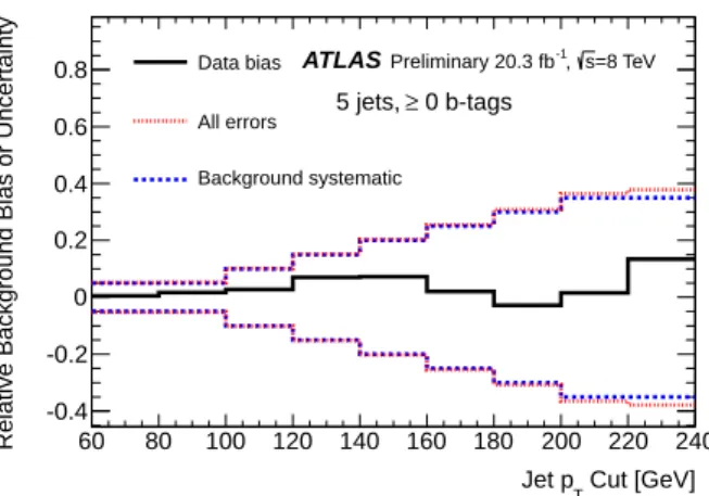
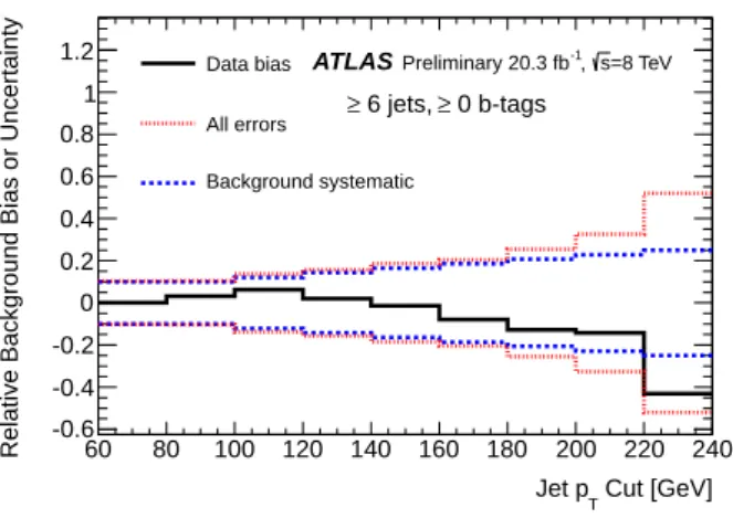
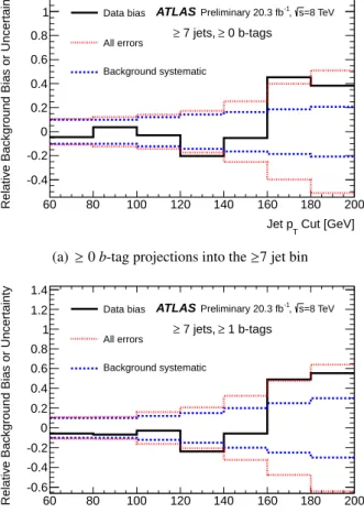
In addition to the systematic uncertainty on the background normalisation, the statistical uncertainties from the data and MC in the control regions must be taken into account when projecting into the signal regions. A visual representation of the size of the background uncertainties compared with observed biases in the data is shown when projecting from the 3-jet bin into the 5-jet bin in Fig. 9. This bias is defined as the relative di ff erence between the observed data and the predicted background ((expectation - data) / expectation)). Since the 5-jet bin was used as one of the inputs to the determination of the background uncertainties, the discrepancy of the data compared to expectations must be smaller than the systematic uncertainties in these plots by construction. Similar plots for projections into the candidate signal regions, where projections are made across two jet bins into the ≥6 and ≥7 jet bins, are shown in Figs. 10 and 11. In these plots the statistical uncertainties become significantly larger, as expected.

An additional systematic uncertainty is assigned to cover possible contamination of signal in the control regions for the projection. The analysis was rerun with signal injected into the control regions in the data and the backgrounds were re-computed. The resulting bias depends on the signal model and is observed to be less than 5% in all cases. This bias is taken as a systematic uncertainty.

5.2 Uncertainties in the signal expectation

Various uncertainties on the signal expectation are considered with a focus on the jet energy scale and jet

energy resolution, flavour tagging uncertainties, and theoretical uncertainties on the signal modeling.

Cut [GeV]

Jet pT

60 80 100 120 140 160 180 200 220 240

Relative Background Bias or Uncertainty

-0.4 -0.2 0 0.2 0.4 0.6

0.8 ^{Data bias}

All errors

Background systematic

ATLASPreliminary 20.3 fb^-1, s=8 TeV 0 b-tags

≥ 5 jets,

(a)

0

Cut [GeV]

Jet pT

60 80 100 120 140 160 180 200 220 240

Relative Background Bias or Uncertainty

-0.6 -0.4 -0.2 0 0.2 0.4 0.6 0.8 1 1.2 1.4

Data bias All errors

Background systematic

ATLASPreliminary 20.3 fb^-1, s=8 TeV 1 b-tags

≥ 5 jets,

(b)

1

Cut [GeV]

Jet pT

60 80 100 120 140 160 180 200 220

Relative Background Bias or Uncertainty

-1 -0.5 0 0.5 1 1.5 2 2.5

Data bias All errors

Background systematic

ATLASPreliminary 20.3 fb^-1, s=8 TeV 2 b-tags

≥ 5 jets,

(c)

2

Figure 9: Comparisons of the bias between data and expectations in the 5-jet control region are shown,

along with a comparison to the main sources of uncertainty. These figures correspond to the projections

of Fig. 2. The solid black line shows the relative di ff erence between the observed data and the predicted

background. The blue distribution shows the relative systematic uncertainty on the background estima-

tion. The red distribution shows the total uncertainty on the comparison between background and data,

including the background systematic uncertainty and all sources of statistical uncertainties including the

statistical uncertainty on the data to which the background is compared.

Cut [GeV]

Jet pT

60 80 100 120 140 160 180 200 220 240 Relative Background Bias or Uncertainty -0.6

-0.4 -0.2 0 0.2 0.4 0.6 0.8 1

1.2 _{Data bias}

All errors

Background systematic

ATLASPreliminary 20.3 fb^-1, s=8 TeV 0 b-tags

≥ 6 jets,

≥

(a)

0

Cut [GeV]

Jet pT

60 80 100 120 140 160 180 200 220 240

Relative Background Bias or Uncertainty

-1 -0.5 0 0.5 1 1.5 2 2.5

Data bias All errors

Background systematic

ATLASPreliminary 20.3 fb^-1, s=8 TeV 1 b-tags

≥ 6 jets,

≥

(b)

1

6 jet bin

Cut [GeV]

Jet pT

60 80 100 120 140 160 180 200 220 240

Relative Background Bias or Uncertainty

-1 -0.5 0 0.5 1 1.5 2 2.5 3

Data bias All errors

Background systematic

ATLASPreliminary 20.3 fb^-1, s=8 TeV 2 b-tags

≥ 6 jets,

≥

(c)

2

6 jet bin

Figure 10: Similar to Fig. 9, these figures show a comparison of the relative bias between data and

expectations in the ≥ 6-jet region, along with a comparison to the relative systematic uncertainty on the

background and the relative total uncertainty on the comparison between the background and the data.

Cut [GeV]

Jet pT

60 80 100 120 140 160 180 200

Relative Background Bias or Uncertainty

-0.4 -0.2 0 0.2 0.4 0.6 0.8

1 Data bias

All errors

Background systematic

ATLASPreliminary 20.3 fb^-1, s=8 TeV 0 b-tags

≥ 7 jets,

≥

(a)

0

Cut [GeV]

Jet pT

60 80 100 120 140 160 180 200

Relative Background Bias or Uncertainty

-0.6 -0.4 -0.2 0 0.2 0.4 0.6 0.8 1 1.2 1.4

Data bias All errors

Background systematic

ATLASPreliminary 20.3 fb^-1, s=8 TeV 1 b-tags

≥ 7 jets,

≥

(b)

1

7 jet bin

Cut [GeV]

Jet pT

60 80 100 120 140 160 180

Relative Background Bias or Uncertainty

-0.5 0 0.5 1

1.5 _{Data bias}

All errors

Background systematic

ATLASPreliminary 20.3 fb^-1, s=8 TeV 2 b-tags

≥ 7 jets,

≥

(c)

2

7 jet bin

Figure 11: Similar to Fig. 9, these figures show a comparison of the relative bias between data and

expectations in the ≥ 7-jet region, along with a comparison to the relative systematic uncertainty on the

background and the relative total uncertainty on the comparison between the background and the data.

The jet energy scale uncertainty is determined from a variety of studies in simulation, in-situ mea- surements, and test beam data [24, 49]. This accounts for uncertainties in the detector modeling as well as the parton-shower and flavour modeling of the jets. Uncertainties in the jet resolution [44] are deter- mined from an in-situ measurement of the jet response asymmetry in dijet events. These uncertainties were applied to this search by smearing the jet energies in the signal simulation according to these un- certainties.

Flavour tagging efficiencies are calibrated and uncertainties are determined individually for b-jets, jets that originate from a c-quark, and jets originating from a light-flavour quark. The b-tagging e ffi cien- cies and uncertainties were determined from measurements in muon-enriched dijet data [46] and in t¯ t data [45]. The c-tagging efficiencies were determined from analysis of D

hadrons in muon-enriched dijet data. Finally, the light-flavour tagging e ffi ciencies were determined from the study of tagged jets with tracking or vertex-mass characteristics that were inconsistent with those of the decays of real heavy- flavour hadrons in dijet events [48]. The uncertainties for real b-jets contribute the most to the tagging uncertainties on the signal expectation in this search.

The signal acceptances rely upon leading order (LO) simulation samples which use the LO PDF set CTEQ6L1. The uncertainties on the acceptance are determined by comparing a wide variety of PDF sets to cover the disagreements between them. These are determined separately from the PDF uncertainties on the inclusive signal cross-section which are considered to be uncertainties on the theory model that is compared with the results of the limit setting procedure. In contrast, PDF uncertainties on the acceptance are propagated directly into the limit setting procedure itself.

To determine the PDF systematic uncertainties on the signal acceptance the samples which were simulated using the CTEQ6L1 PDF set are taken as a baseline. The MSTW2008lo eigenvector set [50]

was used to determine 68% confidence-level bands at LO, consistent with the LO generator. Events are reweighted to match the appropriate probabilities to agree with each PDF set keeping the inclu- sive cross-section fixed in each case and allowing only the acceptance to float. Comparisons are also made to the PDF set NNPDF23 [51], determined at next-to-next-to-leading-order (NNLO). When ac- ceptances are compared across all of these PDFs, it is seen that the acceptances are generally the largest for MSTW2008lo and the smallest for CTEQ6L1. An uncertainty envelope of possible acceptances is therefore formed such that it spans the total range from the smallest of the acceptances predicted by any PDF to the largest (including what is allowed at ± 1 σ level by the MSTW2008lo uncertainty). One-half of the full width of this envelope is chosen as the PDF acceptance uncertainty for this analysis, while the central-value acceptance that is used for the final measurement is chosen to be the midpoint of the envelope.

The nominal cross-section and the uncertainty are taken from an envelope of cross-section predic- tions using different PDF sets and factorisation and renormalisation scales, as described in Ref. [52].

These cross-sections are calculated to next-to-leading order in the strong coupling constant, adding the resummation of soft gluon emission at next-to-leading-logarithmic accuracy (NLO + NLL) [28–32]. This uncertainty is not used when setting limits on the allowed gluino cross-section. Instead the resulting limits on allowed gluino masses from this analysis are quoted only for an inclusive cross-section that is one sigma lower than the nominal calculated value of the inclusive cross-section.

A 2.8% uncertainty on the luminosity determination is included for all signal and background MC- simulation samples. The uncertainty is derived, following the same methodology as that detailed in Ref. [27], from a preliminary calibration of the luminosity scale derived from beam-separation scans performed in November 2012.

The e ff ects of trigger and pileup modeling on the signal acceptance have been studied and determined

to be negligible. Finally, systematic uncertainties on the signal acceptance from QCD radiation (initial

state and final state radiation) are not considered. The reason for this choice is that there is no SM

process that contains a colour flow similar to the signal in this analysis due to the presence of colour-

epsilon tensors involved in the RPV vertex [53]. As a consequence, the theoretical understanding of the QCD radiation is less developed than for most other processes, and the procedure for determining uncertainties is less clear. Further, it is important to make these results available in a way that allows them to be applied to multi-parton models with a different colour flow. The modeling of colour flow and radiation in the signal samples is therefore considered to be part of the model that is analysed in this paper. When reinterpreting the results for other models, it is therefore necessary to account for any differences in colour flow that may arise.

6 Optimization, Results, and Interpretations

6.1 Optimization and limit setting procedure

The results of this analysis are used to derive model-dependent exclusion limits in the context of RPV SUSY models. All limits are calculated at 95% confidence level (CL) by testing the signal plus back- ground hypothesis using the profile likelihood method with the CL

prescription [54]. Systematic uncer- tainties are treated as nuisance parameters with Gaussian likelihood functions.

The optimization procedure to determine the best signal region for each signal hypothesis was per- formed without considering data in the candidate signal regions. The following variables were allowed to float: the p

cut that is used in selecting jets (from 80 GeV to 220 GeV in 20 GeV steps), the minimum number of required jets (6 or 7), and the minimum number of required b-tags (from 0 to 2). Regions used in the background uncertainty determination as outlined in Section 4 are excluded from the optimization procedure. Optimization was done separately for each gluino mass value (and for each neutralino mass value in the case of the 10-quark model), and for many RPV flavour hypotheses.

From Eq. 1 it is clear that each RPV decay produces exactly two down-type quarks that are of different flavours from one-another and one up-type quark. Since the cross-sections for gluino production are not dependent upon the λ

parameters, it is not possible to directly probe or set limits upon any individual λ

parameters. Instead, results are categorized based upon the probability for an RPV decay to produce a t-quark, a b-quark, or a c-quark. These branching ratios are denoted by BR(t), BR(b), and BR(c), respectively. It should be remembered that both top and charm quarks share the same index i in the λ

, so that only one charm or one top quark can be present in an RPV decay, and BR(t) + BR(c)

≤ 1. Similarly, at most one b quark can be produced in an RPV decay, either from the j index or from the k index.

Results are determined for di ff erent hypotheses on the branching ratios of RPV decays to t, b, c, and light flavor quarks. The selection requirements for the signal regions were optimized separately for each of these hypotheses. When running the optimization, the full limit setting procedure was run under the assumption that the expected number of background events is observed in the data, taking all statistical and systematic uncertainties into account. Some example results of this optimization are shown in Tables 2 through 6. Table 2 shows the optimization results and the comparison of the data with background and predictions for the 6-quark signal models under the assumption that (BR(t), BR(b), BR(c)) = (0%, 0%, 0%). In this simple model, it is equivalent to say that only the term given by λ

is nonzero. Explicitly, this flavour hypothesis forces the RPV decays to result only in light-quarks.

Table 3 shows the same comparisons under the assumption that (BR(t), BR(b), BR(c)) = (0%, 100%, 0%) corresponding to only RPV terms given by λ

and λ

. Finally, Table 6 shows the same comparisons for the 10-quark signal model under the assumption that (BR(t), BR(b), BR(c))=(0%, 0%, 0%), again corresponding to λ

. The optimizations for the full flavour space are dominated by the increased sensitivity from b-tagging for models with heavy-flavour couplings. As expected, as the branching ratio to t, b, or c quarks is increased, the optimization procedure tends to favor signal regions with more b-tags.

Specifically, those models with large quantities of t and b quarks tend to favor selections with at least

two b-tags.

Sample Jet p

cut # jets # b-tags Signal Background Data [GeV]

m

= 500 GeV 120 7 0 600±230 370±60 444

m

= 600 GeV 120 7 0 410 ± 100 370 ± 60 444

m

= 800 GeV 180 7 0 13 ± 4 6.1 ± 2.2 4

m

= 1000 GeV 180 7 0 6.8±2.3 6.1±2.2 4

m

= 1200 GeV 180 7 0 2.7 ± 0.5 6.1 ± 2.2 4

Table 2: Optimization results for the 6-quark model under a variety of gluino mass hypotheses when the RPV vertex has the branching ratio combination (BR(t), BR(b), BR(c)) = (0%, 0%, 0%) corresponding to only RPV terms given by λ

being nonzero. The optimized signal region selection requirements are shown along with the resulting background and signal expectations and the number of observed data events. Quoted errors represent both statistical and systematic uncertainty.

Sample Jet p

cut # jets # b-tags Signal Background Data [GeV]

m

= 500 GeV 80 7 2 1900 ± 400 1670 ± 190 1560

m

= 600 GeV 120 7 1 300 ± 60 138 ± 26 178

m

= 800 GeV 120 7 1 131±25 138±26 178

m

= 1000 GeV 180 7 1 4.4 ± 1.0 2.3 ± 1.0 1

m

= 1200 GeV 180 7 1 1.86 ± 0.31 2.3 ± 1.0 1

Table 3: Optimization results for the 6-quark model under a variety of gluino mass hypotheses when

the RPV vertex has the branching ratio combination (BR(t), BR(b), BR(c)) = (0%, 100%, 0%) corre-

sponding to only RPV terms given by λ

or λ

being nonzero. The optimized signal region selection

requirements are shown along with the resulting background and signal expectations and the number of

observed data events. Quoted errors represent both statistical and systematic uncertainty.

Sample Jet p

cut # jets # b-tags Signal Background Data [GeV]

m

= 500 GeV 80 7 1 4600 ± 800 5900 ± 700 5800

m

= 600 GeV 100 7 1 940±190 940±140 936

m

= 800 GeV 120 7 1 108 ± 18 138 ± 26 178

m

= 1000 GeV 120 7 1 42 ± 6 138 ± 26 178

m

= 1200 GeV 180 7 1 1.3±0.4 2.3±1.0 1

Table 4: Optimization results for the 6-quark model under a variety of gluino mass hypotheses when the RPV vertex has the branching ratio combination (BR(t), BR(b), BR(c))=(100%, 0%, 0%) corresponding to only RPV terms given by λ

being nonzero. The optimized signal region selection requirements are shown along with the resulting background and signal expectations and the number of observed data events. Quoted errors represent both statistical and systematic uncertainty.

Sample Jet p

cut # jets # b-tags Signal Background Data [GeV]

m

= 500 GeV 80 7 2 3600±600 1670±190 1560

m

= 600 GeV 80 7 2 2300±400 1670±190 1560

m

= 800 GeV 120 7 2 94 ± 15 38 ± 17 56

m

= 1000 GeV 120 7 2 37 ± 6 38 ± 17 56

m

= 1200 GeV 140 7 2 5.5±1.0 10±5 18

Table 5: Optimization results for the 6-quark model under a variety of gluino mass hypotheses when

the RPV vertex has the branching ratio combination (BR(t), BR(b), BR(c))=(100%, 100%, 0%) corre-

sponding to only RPV terms given by λ

or λ

being nonzero. The optimized signal region selection

requirements are shown along with the resulting background and signal expectations and the number of

observed data events. Quoted errors represent both statistical and systematic uncertainty.

Sample Jet p

cut # jets # b -tags Signal Background Data [GeV] ( m

, m

) = (400 GeV , 50 GeV) 100 7 0 1400 ± 800 2460 ± 350 2477 ( m

, m

) = (400 GeV , 300 GeV) 80 7 0 9000 ± 4000 17200 ± 2100 15885 ( m

, m

) = (600 GeV , 50 GeV) 100 7 1 510 ± 140 940 ± 140 936 ( m

, m

) = (600 GeV , 300 GeV) 100 7 0 1700 ± 900 2460 ± 350 2477 ( m

, m

) = (800 GeV , 50 GeV) 120 7 1 107 ± 31 138 ± 26 178 ( m

, m

) = (800 GeV , 300 GeV) 120 7 0 380 ± 90 370 ± 60 444 ( m

, m

) = (1000 GeV , 50 GeV) 180 6 0 40 ± 6 170 ± 40 187 ( m

, m

) = (1000 GeV , 300 GeV) 140 7 0 50 ± 13 105 ± 25 107 ( m

, m

) = (1000 GeV , 600 GeV) 180 7 0 10 ± 5 6.1 ± 2.2 4 ( m

, m

) = (1200 GeV , 50 GeV) 180 7 0 1.9 ± 1.0 6.1 ± 2.2 4 ( m

, m

) = (1200 GeV , 300 GeV) 180 7 0 3.2 ± 1.4 6.1 ± 2.2 4 ( m

, m

) = (1200 GeV , 600 GeV) 140 7 0 28 ± 4 105 ± 25 107 able 6: Optimization results for the 10-quark model under a v ariety of gluino mass h ypotheses when the RPV v erte x has the branching ratio combi- (BR( t ), BR( b ), BR( c )) = (0%, 0%, 0%) corresponding to only RPV terms gi v en by λ

being nonzero. The optimized signal re gion selection are sho wn along with the resulting background and signal expectations and the number of observ ed data ev ents. Hea vy fla v our quarks are permitted from the R -parity conserving v ertices present in the cascade decay of the gluino, which may lead to optimal signal re gions that include -tags. Quoted errors represent both statistical and systematic uncertainty .