Institut für Höhere Studien (IHS), Wien Institute for Advanced Studies, Vienna

(1)

Institut für Höhere Studien (IHS), Wien Institute for Advanced Studies, Vienna

Reihe Transformationsökonomie / Transition Economics Series No. 7

Share Equations versus Double Logarithmic Functions in the Estimation of Income, Own- and Cross-Price Elasticities

An Application for Bulgaria

Emil Stavrev, Gueorgui Kambourov

(2)

Share Equations versus Double

Logarithmic Functions in the Estimation of Income, Own- and Cross-Price

Elasticities

An Application for Bulgaria

Emil Stavrev, Gueorgui Kambourov

Reihe Transformationsökonomie / Transition Economics Series^*) No. 7

*) Die Reihe Transformationsökonomie ersetzt die Reihe Osteuropa.

The Transition Economics Series is a continuation of the East European Series.

March 1999

Emil Stavrev

Institute for Advanced Studies Department of Economics

Stumpergasse 56, A -1060 Vienna, AUSTRIA Fax: ++43/1/599 91-163

E-mail: stavrev@ihs.ac.at and

CERGE-EI

Politických V•zÁu 7, CZ-111 21 Prague 1 CZECH REPUBLIC

E-mail: emil.stavrev@cerge.cuni.cz

Gueorgui Kambourov CERGE-EI

Politických V•zÁu 7, CZ-111 21 Prague 1 CZECH REPUBLIC

and

UWO, CANADA

E-mail: gkambour@julian.uwo.ca

Institut für Höhere Studien (IHS), Wien Institute for Advanced Studies, Vienna

(3)

The Institute for Advanced Studies in Vienna is an independent center of postgraduate training and research in the social sciences. The publication of working papers does not imply a transfer of copyright. The authors are fully responsible for the content.

(4)

Abstract

In this paper, we compare the results obtained by using double logarithmic demand functions with the one obtained by using functions that relate budget shares to the logarithms of prices and incomes in order to estimate income elasticities and own- and cross-price elasticities for a number of categories of goods. The share equation functional form allows us to model households which do not purchase all goods and estimate unconditional demands that are of interest for policy purposes. We report income elasticities and own- and cross-price elasticities for eight goods for 1993. We compare these estimates with those obtained by using the double logarithmic demand specification.

Keywords

Own- and cross-price elasticities, income elasticities, unit values, quality effects, transition

JEL Classifications

C39, C51, D12, R22

(5)

Comments

This research was undertaken with support from the European Union´s Phare ACE Programme 1996 (Gueorgui Kambourov P96-6701-F and Emil Stavrev P96-7156-S). We would like to thank Prof.

Lester D. Taylor, Prof. Andreas Wörgötter, and our colleagues at the Center for Economic Research and Graduate Education in Prague, and the Institute for Advanced Studies in Vienna for many helpful comments. All errors, however, are ours.

(6)

Contents

1. Introduction 1

2. Model Description and Estimation Procedure 2 3. The Data 7

4. Results 8

4.1. First Stage 9 4.2. Second Stage 10

5. Conclusion 12 References 13

(7)

I H S — Stavrev, Kambourov / Share Equations versus Double Logarithmic Functions — 1

1. Introduction

It is of great importance for public policy to know how consumers alter their expenditures on goods in response to changes in prices. Thus, the estimation of elasticities has been one of the main trends in applied demand analysis. Since the 1930s (Bergson [1936] and De Wolff [1938]), economists have been constantly improving their methodologies and model specifications in order to extract information on different elasticities from cross-sectional and time-series data.¹ For the estimation of price elasticities, time-series data seemed to be the most useful, and it was deemed quite unfortunate that most of the developing countries lacked such data. Deaton (1987, 1988, 1990), however, introduced a procedure which enables researchers to estimate own- and cross-price elasticities from household budget surveys.

Since such surveys are available for a large number of developing countries, this new approach has an enormous practical application. Another application of this method can be found in Laraki’s (1988) analysis of food subsidies and demand patterns in Morocco.

Most of the countries in transition do not have a long enough record of time-series data to allow the estimation of the price elasticities of certain goods. Nevertheless, for the conduct of fiscal policy  especially during the period when the economy is being restructured  governments need to know the approximate magnitude of the elasticities of some important goods. It is also true that the former socialist countries used to gather reliable and sophisticated household budget surveys. Therefore, it is of great interest to determine whether the proposed methodology could be applied to countries in transition.

The central idea in the analysis is to divide the households geographically into clusters. The prices are assumed to be the same within each of the clusters, so that the effects of income and other demographic factors on unit values can be determined and the variance-covariance matrix of the measurement error estimated. Then, in the second stage, the spatial price variation between the different clusters is used for the estimation of own- and cross-price elasticities for various categories of goods.

Double logarithmic demand functions used in Kambourov and Stavrev (1997) are not only inconsistent with the basic theory, but, more importantly, they do not allow modelling of households which do not purchase all goods (see Plips [1983]). Because of zero consumption, we deleted from 5% to 10% of the sample prior to estimation. This selection may introduce bias. Even if we do not introduce bias by deleting zero purchases, the estimated demand functions are conditioned on positive consumption. The revenue effects of a tax change depend on how total demand is altered and not on whether changes take place at the extensive or

1 An excellent survey of the initial fundamental works in this field is Brown, J., and Deaton, A., 1992, “Surveys in Applied Economics: Models of Consumer Behaviour”, Economic Journal, 82, 1145−^1236.

(8)

2 — Stavrev, Kambourov / Share Equations versus Double Logarithmic Functions — I H S

intensive margins. Consequently, for most policy purposes, the unconditional demands are of interest.

We try to solve the problem discussed above by replacing double logarithmic demand functions with the shares of the goods in the household’s budget. We further include zero purchases in the estimation procedure in order to obtain a better estimate of the unconditional demand systems. For an application of Limited Dependent Variable model to Mexican data as another approach dealing with the problem of zero expenditure, see Jarque (1987).

The paper is organized as follows: in section 2, the model and the estimation procedure are described; in section 3 we describe the data, while section 4 presents the results; section 5 concludes the discussion.

2. Model Description and Estimation Procedure

The data we have are on composite goods such as meat, yoghurt, and salami. Each of these categories contains different goods which are themselves of different levels of quality. The households which participated in the surveys recorded both quantities and expenditures.

Therefore, in the data we see, for example, that a certain household for a certain period of time spent 1000 leva buying 20 kilograms of cheese. Dividing the former by the latter  which would be the unit value of cheese  could be used as an indicator that the price of cheese is 50 leva per kilo. It is then straightforward to derive the own- and cross-price elasticities by running a regression of the quantity purchased on the unit value, income, and several other characteristics.

There are, however, a number of problems with such an approach. Prais and Houthakker (1955) noted that unit values seem to be positively correlated with household income. Quality choice also depends on prices since a change in the price of cheese or any other relevant good might have an influence on the quality of cheese consumed by the households. As a result, the price changes would be different from the unit value changes corresponding to the same changes in the quantity consumed. Therefore, the price elasticities might be exaggerated.

Since, most probably, expenditures and quantities have been measured with errors, measured unit values are likely to be negatively correlated with measured quantities.

We use two regression equations for each of the goods that we consider in our demand system: the share equation and the unit value equation. The quantity demanded and the unit value of the goods in group S consumed by household i that is in cluster c is

(9)

( )

w_S _s _s m_ic _s G_ic _sz p f u

z

zc S G

ic = + + + + c + ic

∑=

α⁰ β⁰ γ⁰ θ

1 8

ln ( )^' ln 0 , (1)

lnµ_s α_s β_sln _ic (γ_s)^' _ic ψ_szln _zc

z

m G p uS

= + + + + ic

∑=

1 1 1

1 8

1 . (2)

In equation (1), wSic is the budget share of good S in household i’s budget. It is defined as expenditure on the good divided by total expenditure, mic. Equation (1) postulates linear dependence of goods share on the logarithm of total expenditure, logarithms of the prices of all goods in the demand system, and a vector of household characteristics Gic. f_S_c is a cluster- specific fixed effect while u_G

ic

0 is the error term.

Equation (2) presents the dependence of the unit value on household income, household demographic characteristics, and the prices in the system. The main idea is that the logarithm of unit value is the logarithm of quality plus the logarithm of price. It means that in the absence of quality effects, unit values would move proportionally with price.

Since the prices are assumed to be the same for all households in cluster c, after subtracting the cluster means from equations (1) and (2) will get rid of the unobservable prices. Thus we obtain

(^w^Sîc ⁻^w^{S c}^⋅ )⁼^β⁰^s⁽^ln^mîc ⁻^ln^m^⋅^c⁾⁺⁽^γ⁰^s⁾^'⁽^Gîc ⁻^G^⋅^c⁾⁺(û^S⁰îc ⁻û^{S c}⁰^⋅ )^, ⁽³⁾ (^ln^µ^Sîc ⁻^ln^µ^{S c}^⋅ )⁼^β¹^s⁽^ln^mîc ⁻^ln^m^⋅^c⁾⁺⁽^γ¹^s⁾^'⁽^Gîc ⁻^G^⋅^c⁾⁺(û^S¹îc ⁻û^{S c}¹^⋅ )^. ⁽⁴⁾

The notation “.” indicates means over all households in cluster c. The parameters β⁰_s in (1) and β¹_s in (2) determine the total expenditure elasticities of quantity and quality. From (2) we have that β ∂ µ

∂

s

S

m

1 = ln

ln . Taking into account that unit value is price multiplied by quality, β¹_s

is the expenditure elasticity of quality. If we denote by ηS the quantity demand elasticity after differentiating (1) with respect to lnm, we obtain

∂

β η β ln

ln w

m w

S S

S

S S

= ⁰ = + ¹ −1. (5)

The last term of equation (5) is obtained by taking into account that the logarithm of the share is the sum of the logarithms of quantity and quality less the logarithm of expenditure. From the above equation we get

(10)

η β β

S S

S

wS

= −1 ¹ +

0

. (6)

Let ηSZ ,ψSZ be elements of matrices of own- and cross-price elasticities of the quantities and unit values respectively. After differentiating (1) with respect to lnpz, we have

∂

∂ln η ψ θ ln

w

p w

S z

SZ SZ

SZ S

= + = ^, ⁽⁷⁾

and

η ψ θ

SZ SZ

SZ

wS

= − + . (8)

Given the assumption that the basic goods which comprise each composite commodity are separable, Deaton (1988) shows that

ψ δ β η η

SZ SZ

S SZ S

= + ¹ , (9)

where δSZ is Kronecker delta. Assuming that (9) holds at the sample means and substituting (6) and (8) in (9), we obtain a relationship that connects quantity and quality own- and cross-price elasticities:

ψ δ

β θ ψ β β

SZ SZ

S SZ

S

SZ

S S S

w w

= +

−

− +

1

1 0

1

( )

. (10)

We define the vector α by

α β

β β

S

S wS S

= − +

1

1 0

1

( ) ^, ⁽¹¹⁾

and then (10) can be rewritten in matrix notation as

Ψ = I + D(α)Θ - D(α)D(w) Ψ , (12)

(11)

where I is the (8x8) identity matrix and D(•) denotes a diagonal matrix with the vector α or vector of goods shares w on its diagonal.

The estimation is done in two stages. In the first stage, we use equations (3) and (4) and apply OLS to each equation. The subtraction of cluster means in equations (3) and (4) removes not only the fixed effects in (3) but also the cluster invariant prices in both equations. Let us denote the residuals from the two sets of first stage regressions as e⁰Sic and e¹Sic. We use them later to obtain consistent estimates of the variance-covariance matrix of the residuals of equations (1) and (2) using the following formulas

~ ( )

σ_SZ _Sic _Zic

i c

n C k e e

00 = − − ⁻1∑∑ 0 0 ^, ⁽¹³⁾

~ ( )

σ_SS^rq _S^p _Sic^r _Sic^q

i c

n C k e e

= − − ⁻¹∑∑ ^, r,q = 0,1, S,Z = 1,8. (14)

where n is the total number of households and n^pS is the number of households with positive consumption for the particular good S. In (13) the summation is taken over all households, while in (14) over households with positive consumption for the corresponding good. It is assumed in (14) that covariances in the unit value equation as well as between unit value and share equations are zero.

The estimated β~⁰_s , β~¹_s , γ~_s⁰ , and γ~¹_s are further used in the second stage of estimation to calculate the parts of mean cluster shares and unit values that are not accounted for by the first-stage variables. Let us define

~ ~

ln ~

y w m G

S c⁰_⋅ = S c_⋅ −βs⁰ _⋅c −γs⁰ 1_⋅c^, ⁽¹⁵⁾

~ ln ~

ln ~

y_{S c}¹_⋅ = µ_{S c}_⋅ −β_s¹ m_⋅_c −γ_s¹G1_⋅_c^. ⁽¹⁶⁾

Define S as the variance-covariance matrix of y¹S.c and R the covariance matrix between y⁰S.c

and y¹S.c by

( )

s_SZ y y

S c Z c

=cov ¹_⋅ , ¹_⋅ , (17)

( )

r_SZ y_{S c} y

=cov ⁰_⋅ , ¹Z c_⋅ . (18)

We denote the covariance matrix of residuals in (13) by Σ. This is the covariance matrix for residuals of the share equations. From (14) when r = q = 1 we obtain estimates for residuals from within unit value equations and denote their variance matrix by Ω. We receive between

(12)

equation variance matrix when r = 1 and q = 0 and denote it by Γ. The last two matrices are diagonal.

Taking probability limits over all clusters of the population versions of (15) and (16), we obtain

S = ΨMΨ^‘ + ΩN^-1p, (19)

R = ΨMΘ^‘ + ΓN^-1, (20)

where M is the variance-covariance matrix of the unobservable price vector,

N^-1p = plimC^-1ΣcD(n^pc)^-1, with D(n^pc) a diagonal matrix formed from the average cluster number for the corresponding goods with positive consumption only, and N^-1 is a matrix constructed using the average cluster number before deleting zero consumption of respective goods. We calculate the matrix Β~according to

( ) ⁽ ⁾

~ ~ ~ ~ ~

Β= S −ΩT_p⁻¹ ⁻¹ R−ΓT⁻¹ , (21)

where (∼) denotes an estimate and the diagonal matrices T and Tp are the sample versions of N and Np. As the sample size goes to infinity and cluster sizes remain fixed, we obtain

( )

p

c

limΒ~ Ψ' Θ'

→∞

= −¹ . (22)

Using (22) and (12) we calculate Θ using the following formula:

Θ = B^’{I - D(α)B^’ + D(α)D(w)}^-1 . (23)

The matrix of price elasticities E, from (8), is {D(w)}^-1Θ - Ψ. After substituting we receive E = { D(w)^-1B^’ - I}{I - D(α)B^’ + D(α)D(w)}^-1 . (24) In order to calculate the estimates of E and Θ we replace in (23) and (24) the theoretical magnitudes with estimates from the first and second stages and sample mean budget shares for the vector w.

(13)

3. The Data

The data is from the 1993 Household Budget Survey for Bulgaria including 2490 households.

The survey records values and quantities for the following eight groups of goods: alcohol, bread, cheese, ground meat, meat, salami, yoghurt, shoes. These categories, however, are aggregated goods, and therefore (1) alcohol includes beer, fruit wines, grape wines, liquors, hard liquors (rum, vodka, brandy, whiskey, cognac, etc.) and rakiya;² (2) bread includes more than ten types of bread and a large variety of bakery products; (3) cheese includes white cheese (sheep, cow, mixed), yellow cheese (spread cheese, smoked cheese, and special brands), sour cream, and ice-cream (all brands); (4) ground meat includes various types of ground meat; (5) meat includes all types of meat; (6) salami includes various types of salami;

(7) yoghurt includes all types of yoghurts; and (8) shoes includes all types of men’s shoes, women’s shoes, and children’s shoes.

The vectors of budget shares are (0.016, 0.027, 0.038, 0.053, 0.016, 0.038, 0.065, 0.015) in 1992 and (0.013, 0.017, 0.032, 0.045, 0.015, 0.038, 0.067, 0.014) in 1993 for yoghurt, shoes, salami, meat, ground meat, cheese, bread, and alcohol. The share of the investigated demand system in the total expenditure of the households was 0.267 in 1992 and 0.241 in 1992.

We have divided the households geographically into clusters. First, the separation was done according to the 28 districts into which Bulgaria was divided in 1993. Additionally, within these regions, we were able to organise the households into clusters using the household code to identify the geographically separated areas. The capital Sofia and another four big cities were divided into clusters as well because of the likely price variation among the different city areas.

Finally, we ended up with 418 clusters with an average size of 5.50 households.

As a proxy for income in the within-cluster regressions, the total per capita expenditure of the household was used. Our share variable is defined as the share of the expenditures for the given good out of total household expenditures. For each household we used the following demographic characteristics: household size and the number of people, normalised for the household size, in the following categories: (1) males below 18 years of age, (2) males ages 19−30, (3) males ages 31−44, (4) males ages 44−59, (5) males above the age of 60, (6) females below 18, (7) females ages 19−30, (8) females ages 31−44, (9) females ages 45−55, and, (10) females above the age of 55.

The survey recorded expenditures for the whole year 1993. However, we had some households that participated for less than 12 months. We dealt with this problem in the following way:

those households which participated for six months or less were deleted from the sample; all relevant variables for the other households were then multiplied by 12/n where n is the number

2 A traditional Bulgarian brandy.

(14)

of months of participation. We do not think that this straightforward correction introduced any bias, since a period of 7 to 11 months is long enough to reveal the annual preferences of the household.

In the first stage, those households that did not consume the corresponding good were removed from the sample when running the unit value regressions for that particular good. The quantity regressions, however, were run with all observations in the sample, including households which consumed zero quantities of the specific good.

4. Results

As noted earlier, the estimation procedure consists of two stages. The demand system that we specified consists of alcohol, bread, cheese, ground meat, meat, salami, shoes, and yoghurt.

The rest of the items in the demand system  except shoes and alcohol  are food products for which it seems reasonable to expect cross-price dependence. Alcohol is included as an important good that is expected to influence consumers’ preferences, while shoes are included in order to capture the effect of luxurious non-food commodities.

We examine the matrix of cross-price effects for evidence of Slutsky symmetry. The symmetry is tasted at the average budget shares. Symmetry will be satisfied if we have

∆ = D w E( ) +D w w( )ε ^' −E D w^' ( )−we D w^' ( ) =0, (25) where E is a matrix of cross-price elasticities and ε is a vector of quantity elasticities. In vec notation the above formula can be written as

δ = vec(∆) = (K - I){I⊗D(w)}vecE^’ + (K - I){D(w) ⊗w}ε = 0 (26)

We obtain an estimate of ∆ from the estimates of E and ε. Since ∆ is the difference between a matrix and its transpose, it has a zero diagonal and an upper right triangle that is minus its lower right triangle. Consequently, only the elements of δ corresponding to the bottom left-hand triangle below the diagonal of ∆ are used for inference. We denote this as δ and the corresponding variance-covariance matrix by V(δ). The Wald test is then given by the following expression:

δ^’ {V(δ)}^-1δ (27)

(15)

The matrix V(δ) is constructed from the elements of V(δ) obtained by using (25) above.³ The value of the Wald statistic for the null hypothesis of symmetry is 75.65, which is greater than the critical value for the chi-squared distribution with sixteen degrees of freedom. The critical value at the 5% level is 28.85. We can conclude that the zero hypothesis of Slutsky symmetry is rejected.

4.1. First Stage

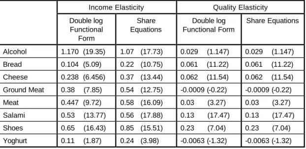
In the first stage we run equations (3) and (4) for each of the eight goods. At this point we are able to estimate the income elasticities and quality elasticities (β¹_s) of the goods (table 1). The t-statistics are given in brackets. We also compare them with the results obtained with the old procedure that uses quantities of the goods consumed instead of their expenditure share.

Table 1: Income and quality elasticities for 1993 obtained with double log and share equations

Income Elasticity Quality Elasticity

Double log Functional

Form

Share Equations

Double log Functional Form

Share Equations

Alcohol 1.170 (19.35) 1.07 (17.73) 0.029 (1.147) 0.029 (1.147) Bread 0.104 (5.09) 0.22 (10.75) 0.061 (11.22) 0.061 (11.22) Cheese 0.238 (6.456) 0.37 (13.44) 0.062 (11.54) 0.062 (11.54) Ground Meat 0.38 (7.85) 0.54 (12.75) -0.0009 (-0.22) -0.0009 (-0.22) Meat 0.447 (9.72) 0.58 (16.09) 0.03 (3.27) 0.03 (3.27) Salami 0.53 (13.77) 0.56 (17.88) 0.13 (17.47) 0.13 (17.47) Shoes 0.65 (16.43) 0.85 (15.51) 0.23 (7.04) 0.23 (7.04) Yoghurt 0.11 (1.87) 0.24 (3.98) -0.0063 (-1.32) -0.0063 (-1.32)

The quality elasticities, of course, are the same since the unit value regressions are the same.

The new approach is in the new quantity equation. The structure of the income elasticities remains the same: alcohol is a luxury good: shoes, salami, meat, and ground meat are relatively elastic; while cheese, yoghurt, and bread have lower elasticities. There are some changes, however. All goods, with the exception of alcohol, have higher income elasticities with the “shares” approach, and this variation is in the order of 50 to 100%. It is worth noting that, contrary to our previous findings, yoghurt displays here a significantly positive income elasticity.

3 For complete and detailed derivation of Wald test for symmetry see Deaton (1990).

(16)

4.2. Second Stage

In the second stage we use the output from the first stage to derive the own- and cross-price elasticities of the goods in the specified demand system. First, we generate the corrected shares and unit values according to (15) and (16) and use them to generate the matrices S and R as given by equations (17) and (18). Second, we generate the Ω^andΓ matrices which would be used to correct for the likely measurement error.

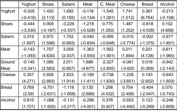
Tables 2 and 3 show the results for 1993 using the double logarithmic functions and share equations respectively, with the t-statistics given in brackets. Despite some slight differences between the results, the elasticities obtained are similar to each other. Half of the estimated coefficients are significant. Three of the own-price elasticities are positive  those of yoghurt, shoes, and salami  but they are not significantly different from zero. The other own-price elasticities are significant and have the expected negative sign.

The own-price elasticities of yoghurt, shoes, and salami remain insignificant no matter which approach is used. Those for bread, cheese, and meat are basically the same. A significant difference is observed in the elasticities of ground meat and alcohol: the one for cheese rises from -1.114 to -2.327 while the one for alcohol falls from -0.708 to -0.248. In general, the results show that ground meat, meat, and cheese exhibit a high price elasticity. Bread, an important good for the Bulgarian consumer, shows a much lower price elasticity. The same applies to alcohol.

(17)

Table 2: The matrix of own- and cross-price elasticities for 1993 using the double log functional form

Yoghurt Shoes Salami Meat G. Meat Cheese Bread Alcohol Yoghurt 0.124 3.293 5.041 -0.900 -3.006 1.190 0.649 -1.369

(0.086) (2.044) (0.504) (-0.258) (-0.700) (0.514) (1.981) (-1.125) Shoes -0.295 -0.050 -0.494 -0.125 0.064 0.148 0.014 0.159

(-4.600) (-0.751) (-1.072) (-0.834) (0.326) (1.426) (0.922) (2.968) Salami 0.891 1.531 0.366 -0.598 0.006 1.076 0.293 -0.686

(3.072) (4.370) (0.177) (-0.846) (0.007) (2.260) (4.110) (-2.799) Meat 0.097 2.457 3.306 -1.547 -2.482 0.878 0.706 -0.735

(0.135) (3.070) (0.664) (-1.890) (-1.150) (0.760) (4.289) (-1.224) Ground 0.378 0.726 1.121 1.770 -1.114 0.633 0.438 -0.661 Meat (0.939) (1.786) (0.404) (1.921) (-1.913) (0.987) (4.798) (-2.001) Cheese 0.832 1.177 2.778 -0.539 -0.528 -1.269 0.451 -0.790

(3.437) (3.922) (1.571) (-0.928) (-0.705) (-3.268) (7.572) (-3.689) Bread 0.454 -0.469 -0.399 0.082 0.890 0.136 -0.530 -0.094

(12.88) (-10.57) (-1.590) (1.042) (8.128) (2.486) (-5.667) (-3.314) Alcohol 0.980 -0.495 0.250 -0.835 0.130 0.312 -0.020 -0.708

(4.452) (-1.938) (0.158) (-1.680) (0.189) (0.891) (-0.348) (-3.917)

Table 3: The matrix of own- and cross-price elasticities for 1993 using the “shares”

approach

Yoghurt Shoes Salami Meat C. Meat Cheese Bread Alcohol Yoghurt -0.005 1.420 1.692 -0.118 -1.545 1.741 0.367 -0.213

(-0.418) (2.113) (0.155) (-0.134) (-1.281) (1.012) (6.754) (-0.158) Shoes -0.444 0.909 -3.229 -1.218 0.775 1.487 -0.618 0.102

(-3.530) (-0.187) (-0.337) (-0.528) (1.250) (1.252) (-0.538) (4.658) Salami 0.319 0.972 1.752 -0.045 -0.495 -0.015 -0.002 -0.677

(1.697) (1.598) (0.693) (-0.834) (-0.648) (-0.774) (-1.375) (-1.851) Meat -0.143 1.707 3.059 -1.363 -1.952 0.211 0.201 -0.611

(-1.093) (4.630) (2.437) (-3.593) (-1.901) (1.894) (4.128) (-1.965) Ground -0.145 1.085 2.011 1.686 -2.327 -0.061 0.018 -0.942 Meat (-0.341) (2.563) (0.857) (4.677) (-2.855) (-0.620 (0.369) (-2.143) Cheese 0.357 0.928 2.833 -0.189 -0.738 -1.228 0.193 -0.643

(4.271) (2.883) (1.914) (-1.411) (-1.630) (-3.651) (2.602) (-1.603) Bread 0.769 -0.751 -1.118 0.130 1.298 0.754 -0.404 0.070

(2.59) (-2.631) (-1.658) (2.688) (4.532) (2.498) (-2.047) (-0.743) Alcohol 0.815 -1.066 -0.131 -0.296 0.376 -0.553 0.123 -0.248

(1.721) (-1.925) (-0.217) (-4.001) (0.427) (-0.440) (-0.289) (-2.659)

(18)

The cross-price elasticities are also similar to each other. The main differences worth noting are that, while the old approach shows that salami is a substitute to cheese and bread and ground meat is a substitute to bread, the “shares” approach reveals insignificant cross-price elasticities.

The following patterns in the cross-price elasticities are observed. Cheese, bread, and alcohol are substitutes for yoghurt. All goods, with the exception of bread and alcohol, are substitutes for shoes. If shoes are truly a proxy for luxury goods, then this result implies that in 1993 the prices of luxury goods were influencing the decision-making of the Bulgarian consumer. The 1993 pattern for salami, meat, and ground meat is different from that of 1992. An increase in the price of salami and meat forces people to switch to cheaper ground meat. An increase in the price of ground meat, however, decreases the consumption of salami and meat, since people cannot switch to these more expensive products and thus stop consuming them altogether.

5. Conclusion

In this paper we replace the double logarithmic demand functions used in our previous work with functions that relate budget shares to the logarithms of prices and incomes in order to estimate income elasticities and own- and cross-price elasticities for a number of categories of goods. This improvement allows us to model households that do not purchase all goods and estimate unconditional demands that are of interest for policy purposes. We report income elasticities and own- and cross-price elasticities for eight goods for 1993. We compare these estimates with those obtained using the double logarithmic demand specification. The estimated elasticities are similar to each other, which implies that both methods are suitable for empirical work on price elasticities in transition economies. The obtained values of the own- and cross-price elasticities are plausible. Results obtained in this work may be further used for policy decisions concerning taxation issues and inequality analysis.

(19)

References

1. Deaton, A. (1987): “Estimation of Own- and Cross-Price Elasticities from Household Budget Data”, Journal of Econometrics, 36, 7−30.

2.  (1988): “Quantity, Quality and Spatial Variation of Price”, The American Economic Review, Vol. 78, No. 3, 418−430.

3.  (1990): “Price Elasticities From Survey Data: Extensions and Indonesian Results”, Journal of Econometrics, 44, 281−309.

4. Deaton, A. and J. Muellbauer (1986):, Economics and Consumer Behaviour, Cambridge University Press.

5. Jarque, C. M. (1987): “An Application of LDV Models to Household Expenditure Analysis in Mexico”, Journal of Econometrics 36, 31−53.

6. Stavrev, E. and G. Kambourov (1998): “Estimation of Income, Own- and Cross-Price Elasticities: an Application for Bulgaria”, mimeo.

7. Laraki, K. (1988): “The Nutritional, Welfare, and Budgetary Effects of Price Reform in Developing countries: Food Subsidies in Morocco”, Welfare and Human Resources Unit, The World Bank, Washington, DC.

8. Magnus, J. R. and H. Neudecker (1986): “Symmetry 0-1 Matrices and Jacobians: A Review”, Econometric Theory, 2, 157−190.

9. Phlips, L. (1983): Applied Consumption Analysis, North-Holland.

10. Pollak, R. A. and Wales, Terence J. (1992): Demand System Specification and Estimation, Oxford University Press.

11. Prais, S. J. and H. S. Houthakker (1955): The Analysis of Family Budgets, Cambridge University Press.

12. Timmer, C. P. (1981): “Is there “Curvature” in Slutsky Matrix?” Review of Economics and Statistics 63, 395−402.

13. Timmer, C. P. and H. Alderman (1979): “Estimation Consumption Parameters for Food Policy Analysis”, American Journal of Agricultural Economics, 61, 982−987.

14. Van de Walle, D. (1988): “On the Use of the Susenas for Modelling Consumer Behaviour”, Bulletin of Indonesian Economic Studies, 24, 107−122.