Limit on B

(1)

ATLAS-CONF-2013-076 18July2013

ATLAS NOTE

ATLAS-CONF-2013-076

July 16, 2013

Limit on B

⁰_s

→ µ

⁺

µ

⁻

branching fraction based on 4.9 fb

⁻¹

of integrated luminosity

The ATLAS Collaboration

Abstract

This note documents the ATLAS analysis searching for B⁰_s → µ⁺µ⁻ decays with an integrated luminosity of 4.9 fb⁻¹, corresponding to the full 2011 proton-proton dataset. This analysis supersedes the previous result based on 2.4 fb⁻¹. We derive a limit on B(B⁰_s → µ⁺µ⁻)<1.5 (1.2)×10⁻⁸at 95% (90%) CL.

Reproduction of this article or parts of it is allowed as specified in the CC-BY-3.0 license.

(2)

1 Introduction

Flavour changing neutral current processes are highly suppressed in the Standard Model (SM), and therefore their study is of particular interest in the search for new physics. The SM predicts the branching fraction for the decay B⁰_s → µ⁺µ⁻ to be extremely small: (3.23 ±0.27)×10⁻⁹ [1] (for complementary SM estimations see Refs. [2, 3, 4]). Due to the finite decay-width difference of the B⁰_s system [5]

the experimental result needs to be compared to the time-integrated branching fraction of B⁰_s → µ⁺µ⁻ (3.54± 0.30)×10⁻⁹ [6]. The branching fraction might be substantially enhanced by non-SM heavy particles in the loop diagrams contributing to the amplitude. Upper limits on this branching fraction have been presented by the collaborations D0 [7], CDF [8] and CMS [9]. The LHCb collaboration recently reported first evidence for the B⁰_s→µ⁺µ⁻decay withB(B⁰_s →µ⁺µ⁻)=(3.2^+1.5₋_1.2)×10⁻⁹[10].

The first analysis of the B⁰_s → µ⁺µ⁻ channel by the ATLAS collaboration [11] has been released using half of the 2011 ATLAS dataset (2.4 fb⁻¹). This note represents an update to the full 2011 ATLAS dataset doubling the available event statistics to the total integrated luminosity of 4.9 fb⁻¹.

The analysis follows the strategy detailed in [11] with additional improvements which include an im- proved event reconstruction of the whole ATLAS 2011 data sample, the use of bb continuum background Monte-Carlo events for the training of the multivariate classifier, an unbinned maximum likelihood fit in two dimensions to extract the yield in the reference channel and a correction for the J/ψpolarisation effect missing in standard Pythia[12] Monte Carlo generation.

The analysis is based on events selected with a di-muon trigger and reconstructed in the ATLAS inner tracking detector and muon spectrometer [13]. After the first 2.4 fb⁻¹ of data recorded in 2011, the di-muon triggers relevant to this analysis changed. A dedicated study confirmed that the implications of this modification are negligible for this analysis. Details of the detector, the trigger and datasets are discussed in Section 2, together with the preselection criteria.

The B⁰_s →µ⁺µ⁻branching fraction is measured with respect to the prominent reference decay B^±→ J/ψK^±in order to minimise systematic uncertainties in the evaluation of the efficiencies and acceptances, without increasing the statistical uncertainties. The branching fraction can be written as

B(B⁰_s→µ⁺µ⁻)=B(B^±→J/ψK^±→µ⁺µ⁻K^±)×

fu

fs × _N^N_J/ψK±^µ⁺^µ− × ^A_A^J/ψK±_µ+µ−

ǫ_J/ψK±

ǫ_µ+µ− , (1)

where the right-hand side includes the B^±→J/ψK^±→µ⁺µ⁻K^±branching fraction, the relative b-quark hadronisation probability fu/fsof B^±and B⁰_staken from previous measurements [14, 15], the event yields after background subtraction, and the acceptance and efficiency ratios. Equation 1 is independent from any luminosity term because we use identical data samples for both the signal and the reference channels.

This note refers to the single-event sensitivity (SES), that is the B⁰_s → µ⁺µ⁻ branching fraction corresponding to one observed signal event in the data sample:

B(B⁰_s →µ⁺µ⁻)= Nµ⁺µ⁻×SES, (2) where Nµ⁺µ⁻is the number of observed events for B⁰_s →µ⁺µ⁻.

A blind analysis was performed where the data in the di-muon invariant mass region 5066 to 5666 MeV were removed from the analysis until the procedures for event selection, signal and limit extractions were completely defined. Sections 2.2 to 2.6 discuss the variables used in the event selection, Monte Carlo (MC) tuning, the background studies, and training of the multivariate classifier used to discriminate between signal and background. The final selection is obtained by an optimisation procedure described in Section 2.7. The ingredients necessary to evaluate the SES are detailed in Section 3. In particular, the relative efficiency and event yields in the reference channel are discussed in Sections 3.2 and 3.3, respectively. Section 4 is devoted to the contributions to the systematic uncertainties. Finally, the signal

(3)

extraction is discussed in Section 5 with the corresponding limit on the branching fraction presented in Section 5.3.

According to the SM, the branching fractionB(B⁰ →µ⁺µ⁻) is predicted to be about 30 times smaller thanB(B⁰_s →µ⁺µ⁻). Therefore, despite the increased B⁰_s→µ⁺µ⁻SES of approximately a factor four due to larger hadronisation probability for B⁰and possible enhancements due to new physics, the sensitivity to this channel is beyond the reach of the current analysis. Hence only a limit on B(B⁰_s → µ⁺µ⁻) is derived by assumingB(B⁰→µ⁺µ⁻) to be negligible.

2 Event Reconstruction and Signal Selection

2.1 The ATLAS Detector

The ATLAS experiment [13] at the LHC is a general purpose particle detector covering almost the full solid angle around the pp collision point with layers of tracking detectors, calorimeters and muon track- ing chambers. The measurement presented here is mainly based on the Inner Detector (ID) and the Muon System (MS).

The ID consists of a silicon pixel detector, surrounded by a silicon strip detector (SCT) and a tran- sition radiation tracker (TRT), embedded in a 2 T axial magnetic field. Charged particle trajectories are measured for|η|< 2.5¹. Enclosing the calorimeter, the MS has a toroidal magnetic field and contains a combination of monitored drift tubes and cathode strip chambers, capable of measuring muon trajectories in a range of|η|<2.7. Muons are triggered by resistive plate chambers (for|η|<1.05) and thin gap chambers (for 1.05<|η|<2.4) with coarse resolution, but fast response time.

The ATLAS detector uses a three-level trigger system, consisting of a hardware-based Level-1 trigger and a software-based Level-2 trigger and Event Filter. The specifics of the trigger selection will be given in the following section.

2.2 Data and Monte Carlo

This analysis uses 4.9 fb⁻¹of data taken at pp-collisions at √

s=7 TeV collected by the ATLAS detector in 2011. Data are only used if the ID and MS subsystems were fully operational and the LHC proton beams were stable.

Monte Carlo events were generated with Pythia 6.4 [12] simulating the following processes: the signal decay channel B⁰_s → µ⁺µ⁻, the reference channel B⁺ → J/ψK⁺ with J/ψ → µ⁺µ⁻, the control channel B⁰_s → J/ψφ with J/ψ → µ⁺µ⁻ andφ → K⁺K⁻, the peaking background B⁺ → J/ψπ⁺ with J/ψ→µ⁺µ⁻, the resonant background decay channels B→hh^′(where h⁽^′⁾stands for a charged pion or kaon) and generic bb→µ⁺µ⁻X sample with two muons in the final state. The latter represents a sample of 2×10⁵ events of the dominant continuum background passing the preselection criteria. It has been used for the Multi-Variate Analysis (MVA) studies, as described in Section 2.7. MC events are filtered before detector simulation to ensure the presence of at least one decay of interest. The B decay products are requested to have|η|<2.5 and p_T >2.5 or>0.5 GeV for muons or kaons, respectively. Since Pythia does not reproduce angular distributions in the B⁺ → J/ψK⁺decay, the B⁺ → J/ψK⁺MC sample has been corrected a posteriori by accepting generated events on the basis of their angular information to reproduce the distribution expected by the J/ψlongitudinal polarisation. The ATLAS detector and its response are simulated using Geant4 [16]. Additional pp interactions in the same and nearby bunch crossings (pile-up) are included in the simulation.

1The pseudo-rapidity isη=−ln(tan(θ/2)), whereθis the polar angle measured from the beam line.The ATLAS coordinate system is described in reference [13].

(4)

A muon trigger [17] is used to select events. In particular, the sample contains events seeded by a Level-1 di-muon trigger which requires a transverse momentum p_T >4 GeV for both muon candidates.

A full track reconstruction of the muon candidates is performed at the second and third trigger levels, where additional requirements on the di-muon invariant mass mµ⁺µ⁻ are applied. The latter loosely select events compatible with decays of the J/ψ (in the mµ⁺µ⁻ range 2500 to 4300 MeV) or B⁰_s (in the mµ⁺µ− range 4000 to 8500 MeV) into a muon pair. Because of the increased instantaneous luminosity and pile-up during the second half of 2011 data-taking period, the Level-1 di-muon triggers with low transverse momentum were marginally redefined [18]. The impact of this modification on the trigger efficiency has been studied with the B⁺ →J/ψK⁺Monte Carlo sample and found to be negligible. The trigger efficiency relative to the event selection described in Section 2.3 is about 52 % and 56 % for the B^±→J/ψK^±and B⁰_s→µ⁺µ⁻decay channels, respectively.

Using the re-weighting method described in [11], the simulated samples are adjusted by an iterative re-weighting procedure: a generator-level (GL) re-weighting based on simulation, followed by a data driven (DD) re-weighting.

The GL re-weighting aims at correcting for the biases induced by the generator-level selection in the relative B⁰_s/B^±acceptance. For this re-weighting, additional MC samples are generated without selection on the final states and over a wider range in the b-quark kinematics:

η^b

< 4 and p^b_T > 2.5 GeV. These samples allow a binned

p^B_T, η^B

map of the efficiencies of the standard generator-level selections to be derived for both the signal and the reference MC. The inverse of such efficiencies are then used to weight events individually, thus correcting the GL filter biases. The respective corrections are applied independently to the simulated signal and reference channel samples.

The DD re-weighting corrects for the residual p^B_T, η^B

differences between data and MC observed after GL reweighting. This procedure uses the comparison of MC events to the sample of B^±→ J/ψK^± decays in collision data. In order not to correlate the re-weighting procedure with the yield measurement, only candidates with odd event numbers in the ATLAS dataset are used to determine the re-weighting procedure, while the remaining sample is used for the yield measurement. In addition, the weights are cross-checked on the B⁰_s → J/ψφcontrol channel. The GL and DD corrections are applied to both the reference and the signal simulated events and only corrected MC samples are used in the following.

2.3 Event Reconstruction and Signal Preselection

Only events containing candidates for B⁰_s → µ⁺µ⁻and B^± → J/ψK^±→µ⁺µ⁻K^± are retained for this analysis. After cutting on the mass of the intermediate resonance (2915 MeV≤ mJ/ψ ≤ 3175 MeV) a preselection is applied. All charged particle tracks reconstructed in the ID are required to have at least one Pixel, six SCT and nine TRT hits. Tracks are required to have|η|<2.5 and p_T >4 GeV (>2.5 GeV) for muon (kaon) candidates. No particle identification is used to distinguish K^±andπ^±candidates. ID tracks matched to reconstructed MS tracks are selected as candidate muons. Decay vertices are formed by combining two or three tracks, depending on the specific decay process. All B meson properties are computed based on the result of the fit of the tracks to the B decay vertex. To reject fake combinations, the fit χ²per degree of freedom is required to be less than 2.0 (85% efficient) for B⁰_s → µ⁺µ⁻ and less than 6.0 (99.5% efficient) for the reference channel. All reconstructed B candidates are required to satisfy p^B_T > 8.0 GeV and|η^B| < 2.5. The primary vertex position is obtained from a fit of charged tracks not used in the decay vertex and constrained to the interaction region of the colliding beams. If multiple candidate primary vertices are present, the one closest in z to the decay vertex is chosen.

Signal and sideband regions are defined according to Table 1. After preselection, approximately 3.9×10⁵ B⁰_s → µ⁺µ⁻ and 2.5×10⁵ B^± → J/ψK^± candidates are obtained in the signal regions. The B⁰_s →µ⁺µ⁻mass resolution in MC is approximately 85 MeV, while for the B^±→J/ψK^±mass resolution in ATLAS data we measure approximately 33 MeV.

(5)

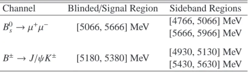
Channel Blinded/Signal Region Sideband Regions B⁰_s →µ⁺µ⁻ [5066, 5666] MeV [4766, 5066] MeV [5666, 5966] MeV B^±→J/ψK^± [5180, 5380] MeV [4930, 5130] MeV [5430, 5630] MeV

Table 1: Definition of blinded (B⁰_s → µ⁺µ⁻) and signal (B^± → J/ψK^±) regions as well as sideband regions used throughout this analysis. The choice for the (B⁰_s → µ⁺µ⁻) signal region is discussed in Sec. 2.7.

2.4 Background Composition

Two categories of background are considered: a continuum with a smooth dependence on the di-muon invariant mass, and sources of resonant contributions from mis-reconstructed decays. Comparisons of data and MC show that the combinatorial background from bb →µ⁺µ⁻X decays provides a reasonable description for the distributions of the discriminating variables for the events found in the sidebands. We use the MC sample of bb→µ⁺µ⁻X events for the training of the MVA classifier (BDT) in order to have the complete data sideband sample for the optimisation and the background interpolation. We verify that this MC sample shows good agreement with the sideband data once some basic kinematic reweighting is applied (see Sec. 2.6). The reweighting technique follows the one used for the signal DD weights (see Sec. 2.2).

Resonant background due to B decay candidates containing either one or two hadrons erroneously identified as muons are expected to contribute inside the signal region. Mis-identification may be due to punch-through of a hadron to the MS or to decays in flight where the muon carries most of the hadron momentum. In either case the hadron fakes the muon signature. The simulation is used to obtain the probability for a hadron to be misidentified as a muon. It is found to be 2.1/4.1/3.3hforπ^±/K⁺/K⁻ respectively, with a relative uncertainty of 20% [19]. The expected event yield for B →hh^′(h⁽^′⁾ being a chargedπor K) is obtained from an estimation of the integrated luminosity, the latest measured branch- ing fractions [20], acceptance and efficiency. This constitutes a nearly irreducible background in this analysis, due to its resemblance to the actual signal. The expected number of events is included both in the optimisation procedure and in the evaluation of the expected background yield for the upper limit extraction.

2.5 Discriminating variables

Table 2 describes the discriminating variables used to separate the signal from the continuum back- ground. To minimise the pile-up dependence, the definition of the isolation observable I0.7is restricted to include only tracks originating from the primary vertex associated with the B decay. This specification makes the selection mostly independent of pile-up as shown in Fig. 1.

These variables are all included in a multivariate classifier, using the TMVA package [21]. Several classifiers were compared and the best performing ones were found to be those based on the Boosted Decision Tree (BDT) algorithm. Several variants of these BDT classifiers were compared to establish the best performing one through the optimisation procedure (see below in Sec. 2.7).

(6)

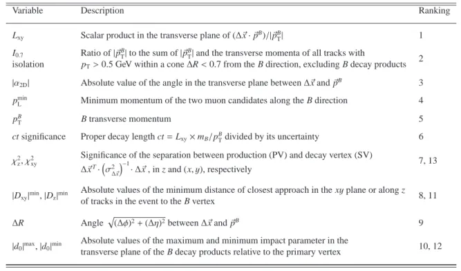
Variable Description Ranking

L_xy Scalar product in the transverse plane of (∆~x·~p^B)/|~p^B_T| 1 I_0.7 Ratio of|~p^B_T|to the sum of|~p^B_T|and the transverse momenta of all tracks with

isolation p_T>0.5 GeV within a cone∆R<0.7 from the B direction, excluding B decay products 2

|α2D| Absolute value of the angle in the transverse plane between∆~x and~p^B 3 p^min_L Minimum momentum of the two muon candidates along the B direction 4

p^B_T B transverse momentum 5

ct significance Proper decay length ct=Lxy×mB/p_T^Bdivided by its uncertainty 6 χ²_z,χ²_xy Significance of the separation between production (PV) and decay vertex (SV)

7, 13

∆~x^T· σ²_∆~_x₋1

·∆~x , in z and (x, y), respectively

|D_xy|^min,|D_z|^min Absolute values of the minimum distance of closest approach in the xyplane or along z 8, 11 of tracks in the event to the B vertex

∆R Anglep

(∆φ)²+(∆η)²between∆~x and~p^B 9

|d0|^max,|d0|^min Absolute values of the maximum and minimum impact parameter in the

10, 12 transverse plane of the B decay products relative to the primary vertex

Table 2: List of the discriminating variables used in this analysis to separate B⁰_s →µ⁺µ⁻signal from continuum background. These variables are based on properties of the decay products, of the reconstructed primary (~xPV) and secondary (~xSV) vertices (separated by∆~x= ~xSV−~xPV), the B meson momentum~p^B and the properties of additional tracks from the underlying event. The last column contains the ranking order of the variable within the BDT.

Mean number of interactions per crossing 0 2 4 6 8 10 12 14 16 18 20 22

Isolation cut efficiency

0 0.1 0.2 0.3 0.4 0.5 0.6 0.7 0.8 0.9

1 isolation with PV association, DATA

isolation without PV association, DATA isolation with PV association, MC isolation without PV association, MC

ATLAS Preliminary = 7 TeV s Ldt = 4.9 fb-1

∫

Figure 1: Efficiency of the cut I0.7 >0.83 as a function of the mean number of interactions per crossing for B^±→J/ψK^±candidate events from data (filled symbols) and MC simulation (empty symbols). The triangles show the efficiency when including all the tracks in the event, while circles show the same efficiency with the isolation definition used in this analysis. Missing MC points at the edges of the distributions are due to the lack of statistics in the MC simulation.

(7)

2.6 Data-MC Comparison

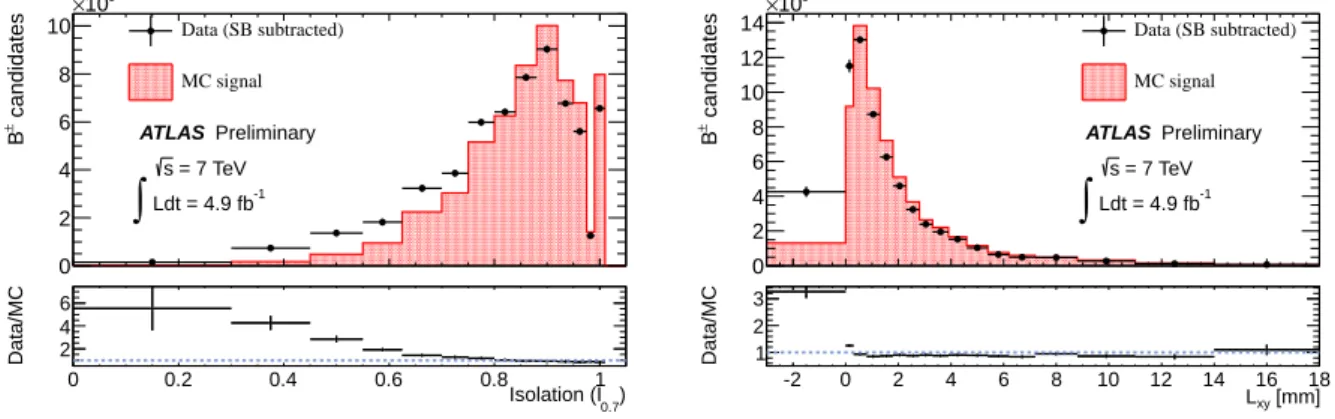
Distributions from B^±→ J/ψK^±events simulated with MC are compared to data after side-band background subtraction for all discriminating variables listed in Table 2 and for variables used in the preselec- tion. Figure 2 shows comparisons for the most powerful separation variables Lxyand I0.7. If we reweight the Lxyvariable to correct for the discrepancy seen in Figure 2 (right), good agreement is found between data and MC for the remaining variables, as shown in Figure 3. This confirms that the discrepancies found in the Lxy variable are not due to background contamination. The data-MC comparison is also cross-checked in the control sample B⁰_s →J/ψφand very good agreement is found. The Lxyreweighting is only used for evaluating the systematic effects associated with the residual data-MC difference. This is discussed in Section 3.2.

Distributions from simulated bb → µ⁺µ⁻X events are compared with the sideband data in Fig. 4.

Events are re-weighted and a selection of Lxy >0.2 mm is applied in order to enhance signal-like events.

This MC sample shows a good agreement and is used for the training of the multivariate classifiers.

0 0.2 0.4 0.6 0.8 1

candidates±B

0 2 4 6 8 10

103

×

Data (SB subtracted) MC signal ATLAS Preliminary

= 7 TeV s Ldt = 4.9 fb-1

∫

0.7) Isolation (I

0 0.2 0.4 0.6 0.8 1

Data/MC 2

4 6

-2 0 2 4 6 8 10 12 14 16 18

candidates±B

0 2 4 6 8 10 12 14

103

×

= 7 TeV s Ldt = 4.9 fb-1

∫

[mm]

Lxy

-2 0 2 4 6 8 10 12 14 16 18

Data/MC 1

2 3

Figure 2: Examples of comparisons of sideband-subtracted data (black dots) and reweighted signal MC (red-filled solid histogram) using B^± → J/ψK^±decays for the two most powerful separation variables:

I0.7 (left) and Lxy (right). Uncertainties are statistical only. The lower graph in each case shows the data/MC ratio.

2.7 Signal Selection Optimisation

The optimisation procedure aims at selecting the best performing BDTs and obtaining the final selection cuts in the BDT output variable q and in the invariant mass window∆m to be applied to our data sample to obtain the best sensitivity to the signal. The signal region is defined as±∆m centred around a mass of 5366.33 MeV.

The optimisation is performed by maximising the following estimator of the separation power of the classifier (for details see [22]):

P= ǫ 1+ √

B, (3)

whereǫ is the signal efficiency and B is the number of background events selected (i.e. the ones with a BDT response above a certain cut value used to select the signal events). Effectively, we are optimising for two sigma background exclusion and two sigma signal discovery. The 2-dimensional optimisation on the BDT output requirement and the signal region width, is performed on the signal MC sample and the odd-numbered sideband data events. The latter represent an independent sample with respect to both the

(8)

0 0.5 1 1.5 2 2.5 3

candidates /0.10 rad±B ²10 103

104

= 7 TeV s Ldt = 4.9 fb-1

∫

| [rad]

α2D

|

0 0.5 1 1.5 2 2.5 3

Data/MC

1 2

0 5 10 15 20 25 30 35 40

candidates /1.00 GeV±B 0 2 4 6 8 10 12 14 16 18 20

103

×

= 7 TeV s Ldt = 4.9 fb-1

∫

[GeV]

L

Pmin

0 5 10 15 20 25 30 35 40

Data/MC

1 2

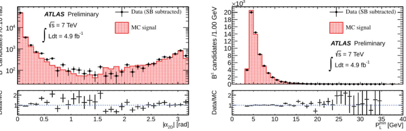
Figure 3: Examples of comparisons of sideband-subtracted data (black dots) and reweighted signal MC (red-filled solid histogram) using B^± → J/ψK^±decays for the next two most powerful separation variables: |α_2D| (left) and p^min_L (right). The MC distributions are also additionally corrected with the weights derived from the Lxyvariable data-MC discrepancy seen in Figure 2. Uncertainties are statistical only. The lower graph in each case shows the data/MC ratio.

Entries

1 10 102

103

104

Sideband data µX µ to b MC b MC signal Preliminary

ATLAS = 7 TeV s

dt = 4.9 fb-1

⋅

∫

L

0.7) Isolation (I

0 0.2 0.4 0.6 0.8 1

Data / MC

0.501 1.52 2.53

Entries

0 1000 2000 3000 4000 5000 6000 7000

8000 Sideband data

µX µ to b MC b MC signal

Preliminary ATLAS

= 7 TeV s

dt = 4.9 fb-1

⋅

∫

L

| [rad]

α2D

|

0 0.2 0.4 0.6 0.8 1 1.2 1.4

Data / MC

0.501 1.52 2.53

Figure 4: Examples of comparisons between sideband data (black dots) and data-reweighted bb → µ⁺µ⁻X MC events (blue solid histogram) for two of the most powerful separation variables: I0.7 (left) and|α_2D|(right). The signal (red-filled solid histogram) is shown for shape comparison. Uncertainties are statistical only. The lower graph in each case shows the data/MC ratio.

training sample (bb→µ⁺µ⁻X MC events) and the sample used to estimate the number of signal events in the signal region (even-numbered sideband data events, see Sec. 5).

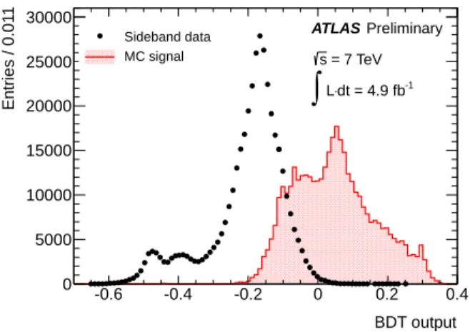
Figure 5 shows the distributions of the chosen BDT output variable for signal MC events and mass sideband data. The analysis described here is based on the observed data distribution.

The odd-numbered event optimisation gives a maximumPvalue of 0.0145. The corresponding final selection cuts on the mass window and the BDT variable are: BDT output>0.118 and|∆m|<121 MeV.

3 Single Event Sensitivity Ingredients

The inputs contributing to the SES (Eq. 1) fall into two categories. The reference channel branching fraction and hadronisation probabilities are taken from external measurements (Section 3.1), while the

(9)

BDT output

-0.6 -0.4 -0.2 0 0.2 0.4

Entries / 0.011

0 5000 10000 15000 20000 25000 30000

Sideband data MC signal

= 7 TeV s

dt = 4.9 fb-1

⋅

∫

L

Figure 5: Distributions of the selected BDT for data-reweighted signal MC events and mass sideband data. The areas are both normalised to the number of entries in the sideband data for shape comparison.

acceptance×efficiency ratio and the reference channel event yield are determined with the 2011 ATLAS dataset (Sections 3.2 and 3.3).

3.1 Reference Channel Branching Fraction and Hadronisation Probabilities

The branching fraction for the reference channel is obtained from the PDG [14] as the product ofB(B^±→ J/ψK^±) = (1.016±0.033)×10⁻³ andB(J/ψ → µ⁺µ⁻) = (5.93±0.06)%. The relative hadronisation probability fu/fsis taken from the best experimental result [15] available: fs/fd = 0.256±0.020 using f_d/f_u = 1. The dependence of the f_u/f_sratio on the decay kinematic is found to be negligible for this analysis [15].

3.2 Evaluation of the Acceptance×Efficiency Ratio

The ratio of the acceptance A and selection efficiencyǫ terms for the B⁰_s → µ⁺µ⁻signal and the B^± → J/ψK^±reference channels, RAǫ = ^A_A^J/ψK±

µ+µ−

ǫ_J/ψK±

ǫ_µ+µ−, is evaluated using Monte Carlo samples. The generator level and data driven corrections as well as the J/ψ polarisation correction are applied to the Monte Carlo samples. The individual A×ǫterms are evaluated as the number of events passing the baseline and optimised selection criteria normalised to the fiducial phase-space volume (p^B_T >8.0 GeV and|η_B|<2.5).

See Table 3 for the central values and their statistical uncertainties.

Channel A×ǫ RAǫ

B⁺ 1.317±0.008% (stat)

0.267±1.8% (stat)±6.9% (syst) B⁰_s 4.929±0.084% (stat)

Table 3: The A×ǫ terms for the B⁺→J/ψK⁺and B⁰_s→µ⁺µ⁻channels and the ratio RAǫ.

Systematic uncertainties are associated with the generator-level and data-driven corrections applied to the Monte Carlo samples and with the observed residual discrepancies between data and Monte Carlo distributions. The impact of both sources has been evaluated by toy experiments. The generator level and data driven corrections have been varied within their uncertainties and the ratio RAǫhas been reevaluated for each toy experiment. The systematic uncertainty on RAǫ due to the residual discrepancies between

(10)

data and Monte Carlo distributions has been estimated by folding the observed data-Monte Carlo discrep- ancies on the B⁺→J/ψK⁺channel as additional weights into the Monte Carlo samples and assigning the change in the value of RAǫas systematic uncertainty. The change in A×ǫis highly correlated between the signal and the reference channels and almost cancels out in the ratio. This is true for all but the isolation variable. The latter has been considered separately, as it depends on the B flavour produced and so sep- arate evaluations have to be performed for the B⁺of the reference channel and the Bsof the signal. For this reason, the estimate of the data-MC discrepancy on the signal for the isolation variable is taken from the B⁰_s→ J/ψφcontrol sample. The total systematic uncertainty on RAǫamounts to∆RAǫ/RAǫ =±6.9%

while the statistical uncertainty due to the finite size of the Monte Carlo sample is±1.8% as summarised in Table 3 (see also Section 4).

3.3 Yield Extraction for the Reference Channel

The reference channel yield NJ/ψK^± is determined from a multi-dimensional unbinned extended maxi- mum likelihood fit to the distribution of the invariant-mass mµ⁺µ⁻K^±of theµ⁺µ⁻K^±system and its event- by-event uncertaintyδmµ⁺µ−K^±, performed in the mass range 4930 – 5630 MeV. The uncertaintyδmµ⁺µ−K^±

on the reconstructed mass is propagated from the uncertainty on the B-candidate vertex fit. To avoid any bias from the DD re-weighting of the Monte-Carlo samples discussed in Section 2.2, only even-numbered events are used in the extraction of the B^± → J/ψK^± yield. Two independent fit strategies based on RooFit [23] are used and the results are combined. The B^± signal mass distribution is modelled by a Gaussian distribution in the first fit and by two Gaussian distributions with equal means in the second.

The background is modelled by a sum of: (a) an exponential function for the continuum combinatorial background; (b) a complementary error function (which is multiplied by a complementary error function in the second fit) describing the low-mass (m < 5200 MeV) contribution from partially reconstructed decays; and (c) a Crystal Ball function [24, 25, 26] with event-by-event uncertaintiesδmµ⁺µ−K^± for the background from B^± → J/ψπ^± decays. The distributions of the event-by-event uncertaintyδmµ⁺µ⁻K^±

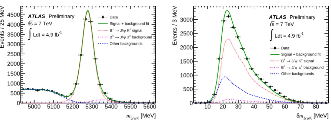
are modelled using a non-parametric kernel estimate [27]. in the first fit, while the second fit utilises a parametric function given by a combination of polynomial and exponential terms. While the first fit uses Monte Carlo events only to model the δmµ⁺µ⁻K^± shapes for the signal and the background from B^±→J/ψπ^±decays, the second implementation constrains the shapes of the signal, of the B^±→J/ψπ^± background and of the partially reconstructed decays by a simultaneous fit to both the data and the corresponding distributions from Monte Carlo events. Figure 6 shows the distributions for the invariant-mass mµ⁺µ⁻K^±and its uncertaintyδmµ⁺µ⁻K^±and the result of the fit to the selected data sample.

The remaining parameters describing the signal and the background components are determined from the fit. For each fit implementation, systematic uncertainties on the extracted reference-channel yield are estimated by using different models and compositions for the backgrounds. Both fit implementations provide a consistent result for reference channel yield NJ/ψK±. The combined result for NJ/ψK± gives 15 214 even-numbered events with an uncertainty of±1.1% (stat.) and±2.4% (syst.).

4 Systematic Uncertainties

The total systematic uncertainty on the B⁰_s →µ⁺µ⁻branching fraction measurement is reduced thanks to the relative measurement w.r.t. the reference channel B^±→J/ψK^±. The SES (see Eq. 2) and the number of background events in the signal region, which are the main ingredients in the branching fraction extraction, are affected by systematic uncertainties.

The different sources and their contributions to the final systematic uncertainty on the SES are summarised in Table 4.

(11)

[MeV]

ψK

mJ/

5000 5100 5200 5300 5400 5500 5600

Events / 25 MeV

0 500 1000 1500 2000 2500 3000 3500 4000

4500 _Data

Signal + background fit signal K± ψ

→ J/

B±

background π± ψ

→ J/

B±

Other backgrounds

= 7 TeV s

Ldt = 4.9 fb-1

∫

[MeV]

ψK

mJ/

δ

10 20 30 40 50 60 70 80

Events / 3 MeV

0 500 1000 1500 2000 2500 3000

Data

Signal + background fit signal K± ψ

→ J/

B±

background π± ψ

→ J/

B±

Other backgrounds

= 7 TeV s

Ldt = 4.9 fb-1

∫

Figure 6: mµ⁺µ⁻K^±invariant mass spectrum (left) andδmµ⁺µ⁻K^±mass uncertainty distribution (right) from even-numbered events passing all selection cuts. The results from the unbinned maximum likelihood fit are overlaid. The solid green curve is the total fit projection on top of the binned data distribution (black circles). The dotted red curve is the B^± → J/ψK^± signal component, the dash-dotted magenta curve is the background from B^± → J/ψπ^±decays, and the dashed blue curve corresponds to the sum of the partially reconstructed B decays background and the combinatorial background components. The later is strongly suppressed by the optimised selection.

description contribution

PDG branching fractions and f_s/f_d 8.5%

K^±tracking efficiency 5%

vertexing efficiency 2%

K^±charge asymmetry. in B^±→J/ψK^± 1%

B^±→ J/ψK^±yield 2.4%

RAǫ 6.9%

total (comb. in quadrature) 12.5%

Table 4: Summary of the∆SES/SES uncertainty due to the dominant sources of systematic uncertainty on the Single Event Sensitivity of (2.07±2.1% (stat.))×10⁻⁹, see also Table 5.

(12)

The largest contribution to the systematic uncertainty is given by the product of the branching frac- tions with the relative b quark hadronisation probability f_u/f_s, see Section 3.1. The second largest contribution is from the acceptance× efficiency ratio RAǫ (±6.9%) and is dominated by the systematic uncertainties introduced by the residual discrepancies between data and Monte Carlo distributions (see Section 3.2). The next largest contributions are the uncertainties on the absolute K^±tracking efficiency (±5%) due to the reliance on Monte Carlo events for its modelling, the uncertainty on the B^±→ J/ψK^± yield (see Section 3.3) and the relative vertexing efficiency in the signal and reference channels (±2%

from Monte Carlo studies). The latter also accounts for the preselection on the fitχ² whose values dif- fer between the signal and reference channels (see Section 2.3). The uncertainty introduced by the K^± charge dependent reconstruction asymmetry, affecting this analysis due to the use of B⁺→ J/ψK⁺Monte Carlo events for the efficiency evaluation for the B^± → J/ψK^±reference channel signal, is estimated to contribute less than 1%.

The number of background events in the signal region Nbkgis interpolated from the sidebands using a parameter R^obs_bkg, defined as the ratio of the size of the two mass sidebands to the size of the signal region.

The systematic uncertainty on R^obs_bkg has been obtained to be 4% [11], accounting for the effect of the mass dependence of the continuum background and additional background components in the low mass sideband like partially reconstructed B decays. The systematic contribution due to the uncertainty on the amount of resonant background (B→hh^′) is negligible due the very small contribution of N_B_→_hh′ in the signal region.

5 Branching Fraction Limit Extraction

Substituting in Equation 1 the ratio RAǫ from Section 3.2, and the B^±yield from Section 3.3, the SES value is obtained, as shown in Table 5. To extract the upper limit on the B⁰_s → µ⁺µ⁻ branching fraction we apply the ATLAS prescription for the extraction of frequentist limits by means of a standard implementation [28, 29] of the CL_smethod [30].

5.1 Likelihood Definition

The CLsupper limit extraction is based on the likelihood:

L = Poisson(N_{S R}ôbs|ǫB+Nbkg+N_B_→_hh) Poisson(N_{bkg,S B}ôbs |RbkgNbkg)× (4) Gauss(ǫôbs|ǫ, σǫ) Gauss(Rôbs_bkg|Rbkg, σR_bkg)

withBrepresenting the branching fraction of interest, ǫ the inverse of the SES and Nbkg the number of continuum background events in the signal region. The directly measured quantities N_{S R}ôbs (number of even- and odd-numbered observed events in the signal region) and N_{bkg,S B}ôbs (number of even-numbered observed events in the two sidebands) enter the CL_s extraction as observables. The expected ratio of background events in the sidebands to those in the signal region, Rbkgandǫ are treated as nuisance pa- rameters which are constrained to the corresponding observables Rôbs_bkgandǫôbswithin their uncertainties by the Gaussian terms in Eq. 4. The Rôbs_bkgvalue corresponds to half of the ratio of the combined widths of the sideband regions and the total width of the signal region given by∆m. The mean of the signal region Poisson distribution is equal to the sum of the number of B⁰_s signal events given by the product of the branching fractionBand the inverse of the SESǫ, the continuum background Nbkgand the contribution from the irreducible resonant B →hh^′ background N_B_→_hh′. The mean of the Poissonian distribution in the sidebands is equal to the continuum background in the signal region scaled by Rbkg.

(13)

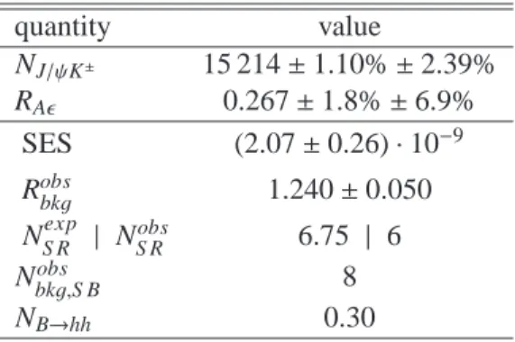
quantity value

NJ/ψK^± 15 214±1.10%±2.39%

RAǫ 0.267±1.8%±6.9%

SES (2.07±0.26)·10⁻⁹ Rôbs_bkg 1.240±0.050 N_{S R}êxp | N_{S R}ôbs 6.75 | 6

N_{bkg,S B}^obs 8

NB→hh 0.30

Table 5: Input values used for the extraction of the upper limits using the CL_smethod. The first two rows summarise the B⁺yield NJ/ψK^±(Section 3.3) and the efficiency ratio RAǫ(Table 3) used in the calculation of the SES values. For the extraction of the expected limit the signal region event count N_{S R}^obs has been set to the background expectation N_{S R}^exp.

5.2 Expected Branching Fraction Limits

Before unblinding the signal region, the expected upper limits are obtained with the input values given in Table 5 by setting the count in the signal region (N_{S R}^obs) equal to the background interpolated from the sidebands plus the small contribution from the B→hh^′resonant background (N_{S R}^exp).

The median expected upper limit forB(B⁰_s → µ⁺µ⁻) is 1.6^+0.7₋_0.4×10⁻⁸ (1.3^+0.6₋_0.4 ×10⁻⁸) at 95% CL (90% CL), where the range encloses 68% of the background-only pseudo-experiments.

We also performed the analysis for the case with multiple mass resolution categories as used in our previous publication [11]. This time, however, no improvement was obtained for the still-blinded analysis, so we use the simpler method described in this note.

5.3 Branching Fraction Limits on Data upper limit (10⁻⁸)

at 95% CL at 90% CL

observed limit 1.5 1.2

expected limit 1.6^+0.7₋_0.4 1.3^+0.7₋_0.4

Table 6: Summary of upper limits on BR(B⁰_s → µ⁺µ⁻) at 95% CL and 90% CL obtained by the CLs

method for the 4.9 fb⁻¹analysis. The expected upper limits from Section 5.2 are shown for comparison, where the±1σranges enclose 68% of the background-only pseudo-experiments.

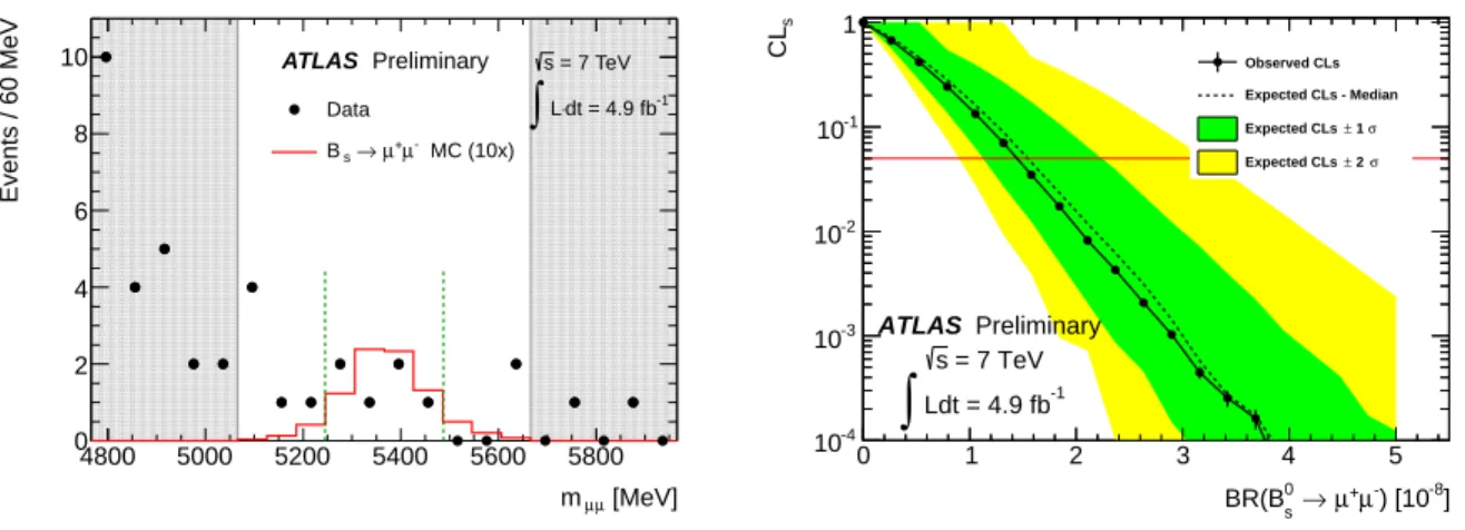
After unblinding, 6 events are counted in the signal region which are set as N_{S R}^obsin the CLslikelihood (Eq. 4). Figure 7 shows the distribution of observedµ⁺µ⁻candidates and the behaviour of the observed CLsfor different tested values of theB(B⁰_s →µ⁺µ⁻), computed with 300 000 toy Monte Carlo simula- tions per point. The observed limit isB(B⁰_s→µ⁺µ⁻)<1.5 (1.2)×10⁻⁸at 95% (90%) CL. The p-values for the background-only hypothesis and for background plus Standard Model prediction are 58% and 24%, respectively. Table 6 summarises the observed and expected upper limits.

(14)

[MeV]

µ

mµ

4800 5000 5200 5400 5600 5800

Events / 60 MeV

0 2 4 6 8

10 _s_{= 7 TeV}

dt = 4.9 fb-1

⋅

∫

L Data

MC (10x) µ-

µ+ s→ B

-8] ) [10 µ-

µ+

→

0

BR(Bs

0 1 2 3 4 5

sCL

10-4

10-3

10-2

10-1

1

Observed CLs Expected CLs - Median

σ

± 1 Expected CLs

σ

± 2 Expected CLs

ATLAS Preliminary = 7 TeV s Ldt = 4.9 fb-1

∫

Figure 7: Left: Invariant-mass distributions of selected candidates in data (dots). The plot also indicates the signal (continuous line) as predicted by Monte Carlo assumingB(B⁰_s →µ⁺µ⁻) =3.5×10⁻⁸(scaled by a factor 10), the signal region (two dashed vertical lines) corresponding to the optimised∆m cut and the sidebands used in the analysis (grey areas). The expected number of B⁰_s →µ⁺µ⁻signal in the signal region is 1.7±0.2 events. The expected background yield per bin in the signal region is 1.7 events.

Right: Observed CLs(circles) as a function of B(B⁰_s → µ⁺µ⁻). The 95% CL limit is indicated by the horizontal (red) line. The dark (green) and light (yellow) bands correspond to the±1σand±2σranges of the background-only pseudo-experiments with the median of the expected CL_sgiven by the dashed line.

6 Conclusions

A limit on the branching fraction B(B⁰_s → µ⁺µ⁻) is set using an integrated luminosity of 4.9 fb⁻¹ collected in 2011 by the ATLAS detector. This analysis supersedes the result obtained earlier with 2.4 fb⁻¹ of integrated luminosity in 2011 [11]. The decay B^±→J/ψK^±, with J/ψ→µ⁺µ⁻, is used as a reference channel for the normalisation of integrated luminosity, acceptance and efficiency. The final selection is based on a multivariate analysis which is now trained on MC, leaving the events in the sidebands to be used for optimisation and background estimation. Furthermore this new results profits from an improved event reconstruction and the use of multi-dimensional unbinned maximum likelihood fits for the extraction of the reference channel yield. We obtain a limit ofB(B⁰_s→µ⁺µ⁻)<1.5 (1.2)×10⁻⁸at 95% (90%) CL.

References

[1] A. J. Buras, J. Girrbach, D. Guadagnoli, and G. Isidori, Eur.Phys.J. C72 (2012) 2172, arXiv:1208.0934 [hep-ph].

[2] A. J. Buras, R. Fleischer, J. Girrbach, and R. Knegjens,arXiv:1303.3820 [hep-ph].

[3] UTfit Collaboration, A. Bevan, M. Bona, M. Ciuchini, et al., PoS EPS-HEP2011 (2011) 185.

[4] CKMfitter Collaboration, J. Charles, O. Deschamps, S. Descotes-Genon, et al., Phys. Rev. D 84 (2011) 033005.

[5] Aaij, R. and others (LHCb Collaboration), LHCb-CONF-2012-002.

(15)

[6] K. De Bruyn, R. Fleischer, R. Knegjens, P. Koppenburg, M. Merk, et al., Phys.Rev.Lett. 109 (2012) 041801,arXiv:1204.1737 [hep-ph].

[7] Abazov, V. et al. (D0 Collaboration), Phys.Lett. B693 (2010) 539–544,arXiv:1006.3469 [hep-ex].

[8] Aaltonen, T. et al. (CDF Collaboration), Phys.Rev.Lett. 107 (2011) 239903,arXiv:1107.2304 [hep-ex].

[9] CMS Collaboration, S. Chatrchyan et al., JHEP 1204 (2012) 033,arXiv:1203.3976 [hep-ex].

[10] LHCb Collaboration, R. Aaij et al., Phys.Rev.Lett. 110 (2013) 021801,arXiv:1211.2674.

[11] ATLAS Collaboration, Phys.Lett. B713 (2012) 387–407,arXiv:1204.0735 [hep-ex].

[12] T. Sjostrand, S. Mrenna, and P. Z. Skands, JHEP 0605 (2006) 026,arXiv:hep-ph/0603175.

[13] ATLAS Collaboration, JINST 3 (2008) S08003.

[14] Particle Data Group Collaboration, J. e. a. Beringer, Phys.Rev. D86 (2012) 010001.

[15] LHCb Collaboration, R. Aaij et al., JHEP 1304 (2013) 001,arXiv:1301.5286 [hep-ex].

[16] GEANT4 Collaboration, S. Agostinelli et al., Nucl. Instr. Meth. A506 (2003) 250303.

[17] ATLAS Collaboration, Eur. Phys. J. C72 (2012) 1849,arXiv:1110.1530 [hep-ex].

[18] ATLAS Collaboration, ATLAS-CONF-2012-099.

[19] ATLAS Collaboration, ATLAS-CONF-2010-075.

[20] Heavy Flavor Averaging Group Collaboration, D. Asner et al.,arXiv:1010.1589 [hep-ex].

[21] A. Hoecker, P. Speckmayer, J. Stelzer, J. Therhaag, E. von Toerne, and H. Voss, PoS ACAT 040 (2007) ,arXiv:physics/0703039.

[22] G. Punzi, eConf C030908 (2003) MODT002,arXiv:physics/0308063.

[23] W. Verkerke and D. Kirkby, tech. rep., SLAC, Stanford, CA, Jun, 2003.

arXiv:physics/0306116.

[24] M. Oreglia, Ph.D. Thesis SLAC-R-236 (1980), Appendix D.

[25] J. Gaiser, Ph.D. Thesis, SLAC-R-255 (1982), Appendix F.

[26] T. Skwarnicki, Ph.D. Thesis, DESY-F31-86-02 (1986), Appendix E.

[27] K. S. Cranmer, Comput.Phys.Commun. 136 (2001) 198–207,arXiv:hep-ex/0011057.

[28] R. Brun, P. Canal, and F. Rademakers, PoS ACAT2010 (2010) 002.

[29] T. Junk, Nucl. Instrum. Meth. A434 (1999) 435–443,arXiv:hep-ex/9902006.

[30] A. L. Read, J. Phys. G28 (2002) 2693–2704.