El Niño / Southern Osillation
in the GFDL-ESM2M
pre-industrial ontrol simulation
Master Thesis written by
Goratz Beobide Arsuaga
Supervised and examined by
Prof. Dr. Mojib Latif
Dr. Tobias Bayr
MATHEMATISCH -NATURWISSENSCHAFTLICHE FAKULTÄTDER
CHRISTIAN-ALBRECHTS-UNIVERSITÄT ZU KIEL
GEOMARHELMHOLTZ - ZENTRUM FÜROZEANFORSCHUNG KIEL
- MARITIME METEOROLOGIE -
Abstrat III
Zusammenfassung IV
Abbreviations VI
1 Introdution 1
1.1 Overviewand motivation . . . 1
1.2 TropialPaimean state . . . 3
1.3 El Niño /Southern Osillation(ENSO) . . . 4
1.3.1 ENSO domains . . . 6
1.3.2 ENSO metris. . . 7
1.3.3 Atmospherifeedbaks . . . 8
2 Data and Methodology 10 2.1 Data . . . 10
2.1.1 GFDL-ESM2M . . . 10
2.1.2 ERA-20C . . . 12
2.2 Methodology . . . 13
2.2.1 Modelmeanstate bias . . . 13
2.2.2 ENSO denition . . . 13
2.2.3 ENSO metris. . . 14
2.2.4 Atmospherifeedbaks . . . 15
2.2.5 DeadalENSO amplitude modulation . . . 16
3 Results 18 3.1 ENSO simulationskills . . . 18
3.1.1 Modelbias inthemeanstate . . . 18
3.1.2 ENSO metris. . . 20
3.1.3 Atmospherifeedbaks . . . 24
3.2 DeadalENSO amplitude . . . 27
3.3 High /LowENSO amplitudeperiods . . . 33
3.3.1 TropialPaimean state . . . 33
3.3.2 TropialPaivariability . . . 36
3.3.3 ENSO metris. . . 38
3.3.4 Atmospherifeedbaks . . . 42
3.4 DeadalENSO amplitude modulation . . . 44
4.2 Disussion . . . 53
4.3 Conlusion. . . 56
List of gures 58
Bibliography 63
Aknowledgement 70
Delaration of andidate 71
The deadal variability of El Niño / Southern Osillation (ENSO) is investigated in the pre-
industrial ontrol runof theGFDL-ESM2M fullyoupled limate model. Overall,the limate
modelhasquite a realisti representation of relevant ENSOproperties: theprobability distri-
bution of Niño3.4 sea surfae temperature (SST) anomalies is positively skewed, the highest
equatorial Pai SSTvariabilityisobservedinborealwinterwiththeorrespondingderease
in variability during spring, and the deadal limate variability shows a shift of the ENSO
spatial pattern. Nevertheless, ompared to the ERA-20Creanalysis produt,themodelshows
problemsmostlimatemodelshave: theanomalousoldequatorialPaiSSTwiththelargest
bias loatedon the eastern side, strong easterlywinds over thewestern equatorial region, the
rising branh of the Walker Cirulation loated too far west and the too strong subsidene
regime east ofthe dateline.
Twomainperiodsofabout60yearswithhighandlowENSOamplitudesareobserved,ran-
gingbetween1.5
◦
Cand0.7
◦
C.Hereitisshown,thattheHighandLowepohshaveremarkably
dierent mean states, whih an explain the dierenes in simulated ENSO amplitudes. The
High epoh is haraterized by a weaker zonal equatorial SST gradient and a warmer Niño3
SST. The less intense Walker Cirulation redues the subsidene branh, and the negative
shortwave (SW) feedbak during El Niño events is extended over the Niño3 domain. The
stronger onvetive response overthe eastern equatorial Pai enhanes the SST variability,
inreasing onsiderably during boreal winter, and the strong non-linearities in atmospheri
feedbaks are kiked forming strong East Pai-like (EP)El Niño events. Hene, theENSO
asymmetry isremarkably inremented.
During the Low epoh, the zonal equatorial SST gradient is inreased with ooler Niño3
SST. The Walker Cirulation is intensied and the subsidene branh over the Niño3 region
is strengthened. The Niño3 domain also oinides with the redution of the negative SW
feedbakduring El Niño events, as well asthe inapability of theatmospheri regime to turn
into a onvetive state, when SST anomalies are turned positive. In addition, the Niño3.4
SST variabilityandthe wind feedbakareonsiderablydereased duringborealwinter. There
are indiationsthat the redued SSTvariability of theLow epoh isaused by thetoo strong
subsidene branh over theNiño3 region, whih restrits theseasonal southward migration of
the Intertropial Convergene Zone (ITCZ), and hampers theevolution of strong EP El Niño
events. However, the onvetive response is maintained over the western equatorial Pai,
outsideofthestrongestmeansubsideneregion,asshownbythehighestnegativeSWfeedbak.
Therefore, during this time period the frequeny of Central Pai-like (CP) El Niño events
is inreased, shifting the ENSOspatial pattern,and reduing SSTvariability inlakof strong
EP El Niños. Correspondingly,the non-linearities between thepositive and negative phasesof
ENSO are redued, diminishing the ENSO asymmetry. In summary, these results show how
important the mean state isfor theENSOamplitude and asymmetry.
IndieserArbeitwurdediedekadisheVariabilitätvonElNiño/SouthernOsillation (ENSO)
mithilfeeinesvorindustriellenKontrolllaufsdesgekoppeltenGFDL-ESM2MKlimamodellsunt-
ersuht.Insgesamt simuliert das Klimamodell die relevanten ENSO-Eigenshaften realistish:
dieMeeresoberähentemperatur (SST) inderNiño3.4-Regionhat eine positive Skewness,die
maximale SST-Variabilität des äquatorialen Paziks ist während des borealen Winters, das
Minimums im Frühling, und in der dekadishen Klimavariabilität zeigt es eine Verlagerung
desräumlihenENSO-MusterszwishenöstlihemundzentralemäquatorialenPazik. Nihts-
destotrotz weist das Modell im Vergleih zur ERA-20C Reanalyse Probleme auf, die viele
Klimamodelle haben: ungewöhnlih kalte SSTs im östlihen äquatorialen Pazik, zu starke
Ostwinde über der westlihen Äquatorregion, ein zu weit im Westen liegender aufsteigender
AstderWalkerZirkulation, und einzu starker,absinkenderAstim östlihen Pazik.
EswurdenzweiZeiträumevonjeweils60JahrenmithohrundniedrigerENSO-Amplituden
identiziert, dieungefähr bei1.5C und 0.7C liegen. Die Epohen hoher und niedriger ENSO-
Amplitud weisen bemerkenswerte Untershiede im mittleren Zustand auf, die erklären kön-
nen,warumdie ENSO-Amplitudsountershiedlih simuliertweird. DieEpohe hoherENSO-
Amplitude ist durh einen verringerten zonalen SST-Gradienten entlang des Äquators und
wärmere SSTs in der Niño3-Region harakterisiert. Die Walker-Zirkulation ist shwäher,
wodurh vor allem der absinkende Ast shwäher ist und dasFeedbak derkurzwelligen Ein-
strahlungsihaufdieNiño3-Regionausweitet. DiestärkereKonvektionüber demäquatorialen
Pazik im Osten verstärkt die SST Variabilität, insbesondere während des borealen Winters,
unddieatmosphärishen Feedbaksweisen starkNihtlinearitäten auf,sodasssihstarkeEast
Pai (EP) El Niño-Ereignisse ausbilden. Entsprehend ist die Asymmetrie zwishen den
ENSOPhasendeutlih verstärkt.
WährendderEpoheniedrigerENSO-Amplitude dagegenistderzonaleSST-Gradient ent-
lang des Äquators verstärkt und weist eine kältere SST in der Niño3-Region auf. Die At-
mosphäre reagiert darauf mit einer Intensivierung der Walker-Zirkulation, insbesondere des
absinkenden Astesüber derNiño3-Region. In dieser Region ist während El Niño-Ereignissen
das negativ kurzwellige Strahlungsfeedbak shwäher, und die vertikalen Wind in 500 hPa
HöhereagierenshwäheraufSST-Anomalien,Dieshatzur Folge,dassdieAtmosphärekeinen
konvektivenZustanderreihenkann,wennSST-Anomalienpositivwerden. Hinzukommt,dass
dieVariabilität derSSTsinderNiño3.4-Region sowiedasWindfeedbakwährenddesborealen
Winters deutlih verringert sind. Es gibt Anhaltspunkte, dass die reduzierte Variabilität der
SSTwährendderEpoheniedrigerENSO-Amplitude durheinenübermäÿigstarkensinkenden
Zweig der Walker-Zirkulation über der Niño3-Region verursaht wird, wodurh die saisonale
südwärtige Migration der Innertropishen Konvergenzzone eingeshränkt wird, was wiederum
dieAusbildungstarkerEPElNiño-Ereignissebehindert. Nihtsdestotrotzwirdeinkonvektiver
ZustandderAtmosphäreüberdemäquatorialenPazikimWestenauÿerhalbderRegionmitder
bak. Aus diesem Grund kommen während der Epohe niedriger ENSO-Amplitude Central-
Pai (CP) EL Niño-Ereignisse wesentlih häuger vor, was das ENSO-Muster in den zen-
tralen Pazik vershiebt und die höhste Variabilität der SST aus Mangel an starken EP El
Niño- Ereignissen verringert. Damit zusammenhängend sind die Nihtlinearität zwishen der
positiven und dernegativen ENSO-Phase reduziert,sodass die Asymmetrievon ENSO gering
ist. Zusammenfassend zeigen diese Ergebnisse, wie wihtig der mittlere Zustand für ENSO-
Amplitude und ENSO-Asymmetrie ist.
SST(A) Sea Surfae Temperature (Anomaly)
T
Oean Subsurfae Temperature
U10(A)
Surfae ZonalWind (Anomaly)
W500(A)
Vertial Windsat 500 hPa height (Anomaly)
NHFS(A)
NetHeat Flux(Anomaly)
LHFS(A)
Latent HeatFlux(Anomaly)
SW(A)
Shortwave (Anomaly)
CLT
TotalCloud Cover
PR
Preipitation
ENSO
El Niño /Southern Osillation
EP
East Pai
CP
Central Pai
TNI
Trans-NiñoIndex
Probability DensityFuntion
ITCZ
IntertropialConvergene Zone
CMIP5
Coupled ModelInteromparison ProjetPhase5
GCM
General Cirulation Model
ESM
Earth SystemModel
Introdution
1.1 Overview and motivation
It isan obviousfatthat ourhumanivilization dependsonthe limate onditions. Although
the soietal, tehnologial and eonomial systems have strongly developed insome ountries,
insulatingagainsttheimpatsoflimatevariability,manyotherdevelopingandunderdeveloped
ountries fae serious vulnerabilitiesrelated to a hanging limate (Handmeret al.,1999). In
fat, while temperate ountries have onverged towardshigh levels of inomeassistedbytheir
limate, tropial ountries inome per apita is saled in muh lower values (Masters and
MMillan, 2001). The inapability of underdeveloped ountries to mitigate limate hazards
ould resultinlarge sale migrationsandonsequentviolent onits,aeting theapparently
safe developed ountries (Reuveny, 2007). Hene, the study of limate variability should be
highly demanded byboth theapparently insulated andvulnerable soieties.
In order to understand and predit global limate variations, the tropial Pai region
playsakeyrole(Wittenbergetal.,2006). Beauseofitslargegeographialextensionandheavy
preipitation, the variability of the tropial Pai limate diretly and indiretly aets the
weather,eosystems,agriulture andhumanpopulationworldwide (Diazand Markgraf,2000;
Hsu and Moura, 2001; Wittenberg et al., 2006). Asa solid example, the El Niño / Southern
Osillation (ENSO) isonsidered to be themost dominant interannuallimate utuation.
ENSO an generally be addressed by old (La Niña) and warm (El Niño) events, whih
aet theeastern-entral equatorial Pai sea surfae temperatures (SST) with negative and
positive anomalies respetively (Philander, 1985). The ENSO phenomenon ontains an irre-
gularperiodiityrangingfrom2to7years,restritingthehighestSSTvariabilitytotheboreal
winter(RasmussonandCarpenter,1982;Bellenger etal.,2014). Itseetsarefeltgloballyvia
atmospheri teleonnetions (Trenberth et al., 1998; Alexander et al., 2002). The 1997-98 El
Niño event in partiular aused billionsof dollars indamages and thousand of livesto be lost
(Kerr,1999; Mphaden, 1999).
ENSO has suered interdeadal modulations in the past, varying its behavior inluding
the frequeny,amplitudeandspatialpattern (Fedorov andPhilander,2000;YehandKirtman,
2005;SunandYu,2009;MPhadenetal.,2011). Infat,apturedbythepaleoreordsweknow
thatthepositiveand negativephasesofENSOhavebeenexitedfor atleastthelast
10 5
yearsand its variability is believed to have hanged onsiderably during the Holoene (Cole, 2001;
Tudhopeetal.,2001;Koutavasetal.,2006;Cobbetal.,2013;MGregoretal.,2013). Similarly,
in thereent past we have been able to observe a deadal shift of the ENSO harateristis.
Forinstane, ainterdeadal shiftofthelate1970slengthenedtheENSOperiodfrom2-4years
to4-6yearswhenomparingthetimeperiods1962-1975 and1980-1993(An andWang,2000).
Nevertheless, due to the short observational reords of tropial Pai limate variability,
longunforedsimulationsofoupledGeneralCirulation Models(GCM)areneessaryinorder
to investigate the natural variability of ENSO on deadal and longer timesales (Wittenberg,
2009;Russonetal.,2014). Forinstane,theGFDLCM2.1pre-industrialontrolrunhasgained
theattentionofmanyauthors,showinglargeunforedmulti-deadalENSOvariabilityhanges
(Wittenberg,2009; Kug et al.,2010; Wittenberg,2015). Themain downside ofthedependene
onoupledGCMsisthatENSOrepresentation suersfrombiasesinthemeanstateaswell as
inthe ENSOdynamis.
AlthoughoupledGCMshaveimprovedsomeoftheENSOharateristisfromtheCMIP3
to the CMIP5 multi-model ensemble reduing by a fator of two the diversity of the ENSO
amplitude,thewind(U10)feedbakandshortwave(SW)feedbakaregenerallyunderestimated
(Bellengeretal.,2014). Hene,theapparentimprovementsoftheENSOamplituderesultfrom
theerror ompensation of ENSO atmospheri feedbaks (Bayr et al., 2018). In addition, the
mainsoureofunrealistiatmospherifeedbaks andhenetheENSOrepresentation hasbeen
attributed to the tropial Pai mean state biases (Dommenget et al., 2014), whih we must
take into onsideration.
The bakground tropial Pai mean state and ENSO harateristi are in fat losely
linked, also indeadal timesales. Whetherthe hanges inthe bakground limatology aet
thedeadal variabilityof ENSO or thehangesin ENSOharateristis aet themean state
ontinues to be ontroversial. Studies using model experiments have proved that the ENSO
amplitudeissensitivetothemeanthermolinedepth(ZebiakandCane,1987;Latifetal.,1993),
to thethermoline tilt(Hu et al.,2013), and tothe mean zonalSST gradient (Knutson et al.,
1997). On theother hand,the interdeadal shift ofthe ENSOasymmetryand spatial pattern
an lead to the modiation of thelimatologial state of thetropial Pai as a residual of
theENSOyle(Ogata etal.,2013). Furthermore,thenon-linearitiesofatmospherifeedbaks
are believed to play a entral role in mean state hanges and the deadal ENSO amplitude
modulation(Atwood et al.,2017;Chen et al.,2017).
Thepresent studyinvestigates thenaturaldeadal variabilityof themainENSO harate-
ristisusinga500yearpre-industrialontrolrunfromthefullyoupledGFDL-ESM2Mlimate
model. AfterexploringthemeanstateandENSObiases,thefousissetontherelationbetween
thedeadal shift of the ENSO statistisand the bakground limatology. Inaddition, speial
attentionhasbeengiventothenon-linearbehavioroftheatmospherifeedbaksduringepohs
ofhighand lowENSO amplitudes.
Throughoutthis work we wouldlike to addressthefollowing questions: Howwell doesthe
modelsimulate ENSO events? Is there any deadal ENSO variability inthe unfored ontrol
run? And ifso, what isits relationshipto thebakground meanstate?
In thesubsequent setions one an readthe desription of the tropial Pai mean state
andENSO. Chapter2 ontains thedataand methodology usedto obtain theresultsshown in
Chapter3. Finally,thesummary,disussion andmain ndings areonluded inChapter4.
1.2 Tropial Pai mean state
Theatmospheriirulationisgenerallyforedbytheinomingsolarradiationandreshapedby
the Earth'srotation. Thedierene inlatitude ofthe inomingsolar radiationisompensated
byasetofdierentirulationells. Inthetropis, thezonallyaveragedmeridionalirulation
between 30
◦
N- 30
◦
S isalledthe HadleyCell(Quan etal., 2004). TheHadley Cellhasapair
ofellularpatternsasendingneartheequatoranddesendingoverthesubtropial area,whih
produes a poleward mass transport in the upper troposphere and equatorward in the lower
troposphere (Bjerknes, 1966). Due to the Earth's rotation, and hene the oriolis eet, the
equatorward owisrediretedwestformingtheeasterlies,ormoreommonlynamed,thetrade
winds (NationalOeani andAtmospheri Administration,2018).
Sinethetropialurrentsrespondto thewind system(Wyrtki,1974), theequatorialeast-
erly winds advet the tropial Pai Oean's surfae westward, piling up the waters on the
westernequatorialsetionandausingathermoline tiltandazonalSSTgradient(Philander,
1981). Theresultleadstoaharaterization ofthewesternPaiequatorialregionbyawarm
pool(i.e. theWestern PaiWarmPool),whose eastward advetion isrestritedbythetrade
winds, and a deep thermoline. On the other hand, the eastern side, enhaned by a shallow
thermoline and anupwelling systemsforedbythe Ekman upwelling, ontains relativelyold
waters forminga old tongue (Jin, 1996). Therefore, although the equatorial inoming solar
radiationiszonallyuniform,theoean-atmospheriproessesleadtoaprodutwhihiszonally
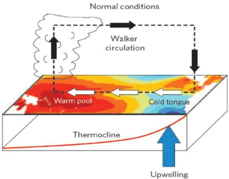
asymmetri (Figure 1.1).
ThezonalasymmetryoftheequatorialPaiisdiretlyrelatedtotheseondell,generally
known as the Walker Cirulation (Figure 1.1). Similarly to the Hadley Cell it is a thermally
diretirulation, onstituted byrisingmotion overthewarmwestern Paiandsinking over
the old waters of the eastern Pai. Its zonal ow is desribed by the westerly winds in
the upper troposphere and the low level winds blowing from the east as part of the trade
winds (Bjerknes, 1969). The prevailing subsidene over the eastern equatorial Pai limits
the formation of deep louds and preipitation. Therefore, the mentioned area is observed
as a highly stable, high pressure zone. In ontrast, unstable atmopsheri onditions with
deep onvetive louds andheavy preipitationarethemain harateristis ofthewestern low
pressure region (Lau K.; Yang S.,2002).
The ollision of the trade winds produes the Intertropial Convergene Zone (ITCZ), a
narrowbandofrisingairandintense preipitation. Thesoureof preipitationisthemoisture
onvergene brought on by the northern and southern hemisphere trade winds towards the
equator (Byrne et al., 2018). As a rst-order approximation, its annual mean positioning
follows thewarm SST and we ould highlight three main regions: a few degrees north of the
equator and hene north of the equatorial old tongue at the entral-eastern Pai, over the
western Pai warm pool, and over thesouth western Pai region, mainly knownas South
Pai Convergene Zone (Yu andZhang,2018).
Nevertheless, the positioning of the ITCZ is not onstant during the year. It follows the
seasonal solaryle, displaingits positionsouthduringborealwinterandnorthduringboreal
summer(Byrneetal.,2018). RelatedtothesouthwarddisplaementoftheITCZ,theequatorial
easterly winds are relaxed and the the eastern equatorial Pai SST are inremented during
Figure1.1: ShematirepresentationofthetropialPai'soeaniandatmospherimeanstates.
Redandblue shadingorrespondtowarmandoldSSTs,respetively. TheWalkerCirulationis
representedbytheblakdashedline, thediretion pointedoutbytheblakarrows. Thewhitearrows
showtheequatorialeasterlywinds,thebluearrowtheupwellingsystemandthesolidredlinethe
depthofthethermoline. Soure: Collinset al.(2010)
1.3 El Niño / Southern Osillation (ENSO)
The El Niño Southern Osillation is a naturally ourring limate variability in the tropial
Pai that warms (ools) the entral-east equatorial region during El Niño (La Niña) events
withafrequenyof2to7years(Bellengeretal.,2014;Capotondietal.,2015). Theatmospheri
manifestationoftheanomalousSSTwarmingandoolingonditionsisthelarge-saleeast-west
sealevelpressureseesawnamed the SouthernOsillation (MPhaden etal., 2006).
A traditional view of an El Niño event starts with the tropial weather noise in boreal
spring, that is, with a set of westerly wind events. It triggers a downwelling oeani Kelvin
wave, deepens the thermoline, redues the upwelling of the old subsurfae waters in the
eastern equatorial Pai and hene, warms the entral-eastern Pai region (Timmermann
etal.,2018). Inautumn, theanomalouswarmSSTdisplaes theupward branh oftheWalker
Cirulation eastward from the Western Pai Warm Pool, leading to the growth of ENSO
(Philander,1983). Theresultisaweakeningofthetradewindsalongtheequatorasthepressure
falls in the eastern Pai and rises in the west. The onseutive eastward transport of the
westPai warm watersensues further positive SSTanomalies (MPhadenetal., 2006). The
peak of the ENSO event ours during boreal winter, oiniding withthe seasonal southward
displaement of the ITCZ (Philander, 1981). The warm waters assoiated with an El Niño
terminating the positive phaseof ENSOand sometimesleading to thetransitionto a LaNiña
state (Bellenger et al.,2014;Timmermann etal., 2018).
Ingeneral,LaNiñaeventsouldbedesribedastheoppositephaseofElNiño,inwhihthe
entral-easternPaiobtainsnegativeSSTanomaliesandthetradewindsandthethermoline
tilt are further inreased. The result is an intensiation of the Walker Cirulation, with an
inreaseofonvetion(subsidene)overthewestern(eastern-entral)Pai(Philander,1985).
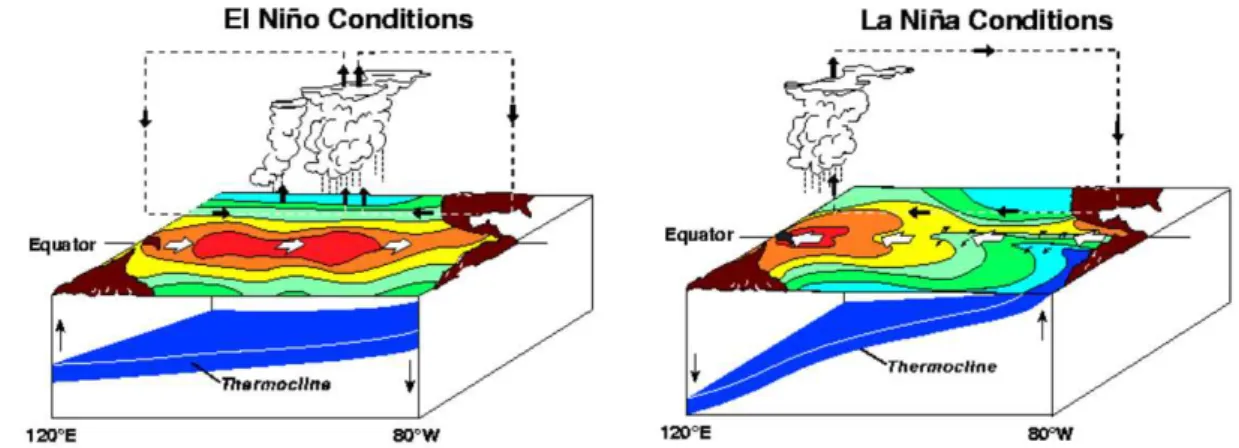
The shemati representation ofEl Niño andLa Niña events isshown inFigure 1.2.
Figure 1.2: El NiñoandLaNiñaonditions: duringanElNiño(LaNiña)eventthethermolineis
attened (tilted),deepening(shoaling)in theeastequatorialPai, warming(ooling)the
entral-easternregions,displaingtheupperbranhoftheWalkerCirulationeastward(westward)
and weakening(strengthening)thetradewinds. Soure: NationalOeani andAtmospheri
Administration(2019)
Although we havealready explained the evolution andharateristis oftheENSO phases
in broadterms, we mustrealize that eah event is singular and no two eventsare alike (Tim-
mermann et al., 2018). ENSO events an dierin amplitude, temporal evolution and spatial
pattern, resulting in a high diversity of episodes with dierent dynamis (Capotondi et al.,
2015). In order to dene a lassiation and luster the large diversity of ENSO events, a
dierentiationbetween theEastPai(EP)or anonialandCentralPai(CP) orModoki
eventshasbeenmade(TrenberthandStepaniak,2001;LarkinandHarrison,2005;Ashoketal.,
2007;Lietal.,2010;KimandYu,2012). EPElNiñoevents,havingtheirpositiveSSTanoma-
lies loatednext totheAmerian ontinent, tendto be ofhigher intensitythan theCPevents
with their anomalousSST visibleoverthe entral equatorial Pai. Inontrast, CPLa Niña
events are usually of larger amplitude than EP La Niña events (Capotondi et al., 2015). In
Figure 1.3the SSTpattern for bothtypesof El Niñoand La Niñaeventsis visible.
Multiple indies have been dened with the objetive to apture spatially varying ENSO
events. Inthe next subsetionswe will introdue thedierent ENSOdomains thathave been
used, and explain some of themetris that aregenerally applied for ENSO researh. Finally,
wewill explainthe fundamentalfeedbaks thatexistwithin theinterationbetween theoean
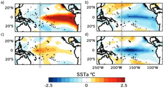
Figure1.3: Spatialpatternoftheseasurfaetemperatureanomalies(SSTA)forspeiwarmand
oldevents: a)East Pai (EP)ElNiñoeventduring 1997-1998,b)EastPai(EP)LaNiñaevent
during2007-2008,)CentralPai(CP)ElNiñoeventduring2004-2005andd)CentralPai(CP)
LaNiñaeventduring1988-1989. Soure: Capotondietal.(2015)
1.3.1 ENSO domains
Severalindiesbasedon SSTanomalies averaged overspei domainshave been employed to
desribe and monitor the SST anomalies as part of the ENSO phenomenon. Those domains
where initially loated over four "Niño" regions by the Climate Analysis Center in the early
1980s(Bamston et al., 1997): Niño1 (90
◦
W eastward, 5
◦
S- 10
◦
S),Niño2 (90
◦
W eastward, 0
◦
-
5
◦
S),Niño3(150
◦
W-90
◦
W,5
◦
N-5
◦
S)andNiño4(160
◦
E-150
◦
W,5
◦
N-5
◦
S).However, sine
theNiño3regionisnotapable todetetthesignalofthe CPEl Niñoeventsverywell(Hanley
et al., 2003; Li et al., 2010), a new domain was needed: theNiño3.4 region (170
◦
W- 120
◦
W
and5
◦
N - 5
◦
S).
Figure1.4: Niñoindex regions: Niño1+2inred(90
◦
W-80
◦
W,0
◦
-10
◦
S), Niño3in blue(150
◦
W-
90
◦
W, 5
◦
N-5
◦
S),Niño3.4(170
◦
W- 120
◦
W,5
◦
N-5
◦
S)dottedandNiño4(160
◦
E-150
◦
W, 5
◦
N -
◦
The updated Niño domains (Trenberth, 2019), as shown in Figure 1.4, are listed in the
following:
•
Niño1+2: The smallest and easternmost of all Niño regionsis a ombinationof initially dierentiatedNiño1andNiño2domains. ItorrespondstotheSouthAmerianoastline,aregion inwhih ENSOwasreognized fortherst time. It extendsfrom90
◦
W- 80
◦
W
and0
◦
- 10
◦
S.
•
Niño3: The most frequently used geographial loation for ENSO monitoring and re- searhing in the past. However, when the omplexity of ENSO ame to light, it wasdisovered that CPENSO events arenot well aptured by theNiño3 region. It extends
from150
◦
W- 90
◦
Wand 5
◦
N- 5
◦
S.
•
Niño3.4:The most sensitive and representative domain to dierent ENSO event avors.It is apable of apturing thesignal of both EP and CP ENSO events. It extends from
170
◦
W- 120
◦
W and5
◦
N - 5
◦
S.
•
Niño4: The westernmost Niño domain. It aptures the SST anomalies in the entral equatorialPai, andextendsfrom 160◦
E - 150
◦
Wand 5
◦
N - 5
◦
S.
1.3.2 ENSO metris
AlthoughENSOisharaterizedbyinterannualtropialPaiSSTanomalyutuations, with
warmEl NiñoandoldLaNiñaevents, thediversityoftheintensity,SSTanomalypatternand
temporal evolution ofindividual episodes leave the produt of a highomplexity phenomenon
(Timmermann et al., 2018). Furthermore, ENSO harateristis suer great modiations on
deadal timesales, altering theENSO regime(An and Wang,2000; Trenberth andStepaniak,
2001;MPhaden etal.,2011;Huetal.,2013,2017). Inthepresentsubsetionwewillintrodue
some of theommonlyusedENSOmetris to understand thetimeevolutionof thementioned
diversity.
InthereentyearswehavebeenabletoobserveashiftintheENSOregime: ompared with
the time period of 2000-2011, tropial Pai interannual variability was onsiderably higher
during1979-1999(Huetal.,2013). Theinreaseinvariabilityisobservedaslargerutuations
from the mean state, that is, pronouned osillations with a larger amplitude, whih an be
alulatedwiththestandarddeviationofaspeivariableoveratimeperiod(Bellenger etal.,
2014;Kimetal.,2014;Wengel etal.,2017). Similarly,beausetheENSOeventsarereferredto
asSSTanomalies,theENSOamplitudemustbeunderstoodastheintensityofSSTvariations
during a speitime frame.
Nevertheless, due to thenon-linear behavior ofENSO, itspositiveand negative phasesare
not symmetri: the amplitude of El Niño events are larger in omparison to La Niña (Tim-
mermann et al., 2018). Hene, the ENSO asymmetry, ommonly omputed as the skewness,
expresses the dierene between El Niño and La Niña event amplitude (Timmermann et al.,
2018).
Temporal hange of the ENSO asymmetry is losely linked to the SST anomaly pattern:
EP ElNiñoeventstendto bestrongerthanCPEl Niñoepisodes, whileEPLaNiñaeventsare
informationaboutthe geographialloation ofthemost anomalousSST,andhene, about the
ourreneof EPor CP events.
Thelast metriisrelatedtotheloserelationbetweentheseasonalyleandENSOevents.
As desribed at the beginning of this hapter, the strongest seasonal equatorial Pai SST
variabilityisrestrited to theboreal wintermonths, beingtheseason during whih theENSO
events tend to peak. The onsequene is thatthe El Niño eventswill grow during theboreal
summerandautumnduetotheinreaseinoean-atmospherioupling(ZebiakandCane,1987;
Wengel etal.,2017)andtheSSTanomalieswillbedampedduringborealspring,aompanied
bytheshoalingofthe easternequatorialthermoline(Harrison andVehi,1999). Thespei
favorable season for the ENSOevent ourreneiswhat we all theENSOphaseloking.
1.3.3 Atmospheri feedbaks
Aswehaveseen,oean-atmosphereouplingandonsequentproessesleadtoENSOevents. In
addition,theENSOdiversitypartlyarisesfrompositiveandnegativeoupledatmosphere-oean
feedbaks(Jinet al.,2006). Thus,thepresentsubsetion willbe dediatedtotheintrodution
ofthemost fundamental interations between the oeanandtheatmosphere.
Apositive(negative)feedbakinvolvesaset ofdierent proessesthatenhane(damp) an
initial perturbation. Present theories usetwo feedbaks to desribethe atmospheriproesses
thatare involved inENSO: thewind (U10) feedbak and the net heat ux(NHFS) feedbak
(Zebiakand Cane,1987;Jinet al., 2006).
The Bjerknes feedbak is the most dominant positive feedbak: the zonal SST gradient
generated by the easterly winds is infat inreased by stronger trade winds, whih in return
will intensify the Walker Cirulation, produing a hain reation. The U10 feedbak, the
atmospheriomponentoftheBjerknesfeedbak,relatestheremotezonalwindsensitivitytoa
given entral-easternequatorial Pai anomalousSSTand itisresponsible forthegeneration
of ENSO events (Bjerknes, 1969; Lin, 2007; Lloyd et al., 2012). As an example, if the zonal
windsarereduedasaresponseofaweakerequatorialSSTgradient,theequatorialKelvinwave
generated bythe wind perturbationwill deepen thethermoline, enhaningfurther heating of
theentral-east SSTand strengthening theinitial redutionof thezonalwinds.
Onthe other hand,a negative NHFS feedbakats asa damping ontheinrementedSST
anomalies and therefore terminates ENSO events (Zebiak and Cane, 1987; Jin et al., 2006).
Inaddition, thenegative NHFSfeedbak an be deomposedinto four individual omponents
(shortwave radiation, longwave radiation, sensible and latent heat uxes), of whih thelatent
heatux(LHFS)andtheshortwave(SW)feedbakdominate(Lloydetal.,2009). Followingthe
previous example, an inrement of the SST over the entral-eastern equatorial Pai will be
followed byathermaldamping,thatis, byaninrementoftheNHFStowardstheatmosphere.
Furthermore,ifstrongpositiveSSTanomaliesswiththeonvetiveresponseoftheatmosphere,
theinrement of the total loud over will redue the inoming SW radiation, reinforing the
dampingof theperturbed SSTand endingthe ENSO event.
Nevertheless, theSWradiationanalsoatasapositive feedbakwhentheSSTanomalies
obtainnegativevalues,thatis,duringLaNiñaevents. Inasubsidenestate,whentheSSTsare
inremented, the destabilization of the atmospheri boundary layerprevents the formation of
an enhanement of the initial perturbed SST (Philander et al., 1996; Xie, 2004). Hene, the
study of theSWfeedbakisnot only relevant for the ENSOphaseloking ortheENSO event
termination, but alsogivesrelevant information about theapability ofthemodelto simulate
the atmospheri swith from subsidene (positive SW feedbak) to onvetive (negative SW
feedbak)state (Bellenger etal., 2014).
Data and Methodology
Inthis hapter we will introdue thedataand the methodology usedin thepresent thesis.
2.1 Data
2.1.1 GFDL-ESM2M
The ore of the present thesis will study a 500 year-long pre-industrial ontrol run simulated
by the oupled arbon-limate Earth System Model from the Geophysial Fluid Dynamis
Laboratory GFDL-ESM2M. The monthly dataused is available on the CoupledModelInter-
omparison Projet Phase 5 (CMIP5) panel and the omplete model desription an be read
inDunne et al. (2012)and Dunneet al. (2013).
Within the CMIP5 model ensemble the pre-industrial ontrol run, often abbreviated as
piControl,isreferredto asthe initialstageofthelongmodelsimulations,aontinuation ofthe
spin-upproess,inwhihtheforing ofgreenhousegases(
CO 2
)ismaintainedtopre-industrial times. Therefore, the unfored simulation will provide us with information about the naturalvariabilityofthe system(European Network for Earth SystemModelling,2019).
The Earth System Models (ESMs) inorporate the interations between the atmosphere,
oean, land, ie and biosphere, inluding proesses, impats and omplete feedbak yles
(Heavens and Mahowald, 2013). The GFDL-ESM2M model has been developed from the
previousClimateModelversion2.1(GFDL-CM2.1),inorporating arbondynamis. Thenew
GFDLgenerationonsistsoftwonewglobaloupledarbon-limateESMs,thepresentESM2M
and the ESM2G, diering exlusively in the oean omponent. Although neither model has
bettergenerisimulationskills,theESM2MmodelisadvisedtobeusedforthetropialPai
irulationand variabilityresearh (Dunne etal., 2013).
A set of variables is usedalong the researh. Besides the sea surfae temperature (SST),
neessaryfor the ENSOanalysis, thesubsurfaetemperatures(T),surfae zonal winds(U10),
vertialwindsat 500 hPaheight (W500),preipitation (PR), totalloud over (CLT) and net
surfaeheat uxes (NHFS)areinorporated inour study inorder to analyzetheatmospheri
state and response. The NHFS's dominant omponents arealso applied: the latent heat ux
(LHFS)andthe shortwave (SW) radiation.
A brief desription of the dierent GFDL-ESM2M omponents and their oupling is pro-
vided next:
a. Atmosphere
The atmospheri omponent is idential to its predeessor CM2.1, the Atmospheri Model
version2(AM2). Ithasa2
◦
latitudinalx2.5
◦
longitudinalhorizontalresolutionwith24vertial
layers. ThegridshemeusedistheDgrid,with3hoursradiationand0.5hourdynamialtime
steps.
b. Oean
The oeanmodelapplied isthe Modular Oean Modelversion4p1 (MOM4p1) set to vertial
pressure layers. The horizontal grid resolution of 1
◦
in latitude and longitude is progressively
nerreahing
1 / 3 ◦
at theequator. Above65
◦
N,a tripolar gridisusedwithpoles overEurasia,
NorthAmeria andAntartia. Inthis ase,themodelonsistsof50 vertiallevels,with10 m
thiknessinthe rst 220 m.
. Land
Integrating the land water, energy, and arbon yles, the Land Model version 3 (LM3.0) is
applied. Thelandwateraountsforamultilayersnowpak,ontinuousvertialsoilwaterwith
saturated and unsaturatedzones, frozen soil water, groundwater disharge, river runo, lakes
as well as lake ie and lake snowpak. Vegetation anopy and leaves are onsidered for the
radiation, the wateryle andarbon dynamis.
d. Sea Ie
The sea iemodel, Sea Ie Simulator (SIS), onsiders full iedynamis, two ie layer and one
snowlayerthermodynamis,andveiethiknessdivision. Theiealbedodierentiates,when
the snow onie is onsidered (0.80) and without snow (0.65), and themelting temperature is
set to 1
◦
C.
d. Iebergs
The originofiebergsisaountedfor,whenthesnowdepth ofLM3.0exeedsaritialvalue.
Then, theexessivesnow pakistransportedto theoean-seaie ompartments byriversasa
Lagrangian partilesdraggedbytheoean,seaie andatmosphere.
e. Coupling
FortheouplingoftheEarthSystemModel'somponentstheFlexibleModelingSystem(FMS)
hasbeenemployed. Theuxesarepassedarosstheomponent's interfaesbytheexhanging
every 0.5hour, while the traer-oupling between theoean andthe atmosphere ours every
2hours.
2.1.2 ERA-20C
The European Centre for Medium-Range Weather Foreast (ECMWF) twentieth entury re-
analysisprodut(ERA-20C)ontainsglobalatmospheridatabetweentheperiodof1900-2010.
Itis therst ECMWF reanalysis preisely onstruted for longterm limate analysis. Hene,
itwill be our referenetoolto keep trakof the GFDL-ESM2M modelrealism.
TheIntegratedForeastSystemversionCy38r1(IFS-y38r1),whihinorporatesanatmos-
pheri general irulation model (AGCM) and a variational sheme, allows a medium range
foreast. IFSouldbedened astheenvironment, wherethedataassimilation andforeasting
ativitiesperformedat ECMWFmeet. Theforeastassimilation issetto 24hour yles,from
whihtheanalysisisobtainedforeahylebyombiningobservationswiththemodelforeast
estimates,initialized fromthe previous yleanalysis.
The model integrations are based on a spetral T159 horizontal resolution, theequivalent
of about 125 km, and 91 vertial levels from 10 m above the surfae up to 1 Pa, that is,
80 km approximately. The presribed model foring, sea surfae temperature and sea ie
onentration, are obtained from HadISST version 2.1.0.0. The solar radiation, tropospheri
and stratospheri aerosols, ozone and greenhousegases foring soures on the other hand are
as speied for CMIP5 experiment. The observations enompasses the atmospheri surfae
pressuredatafromtheInternationalSurfaePressureDatabankversion3.2.6(ISPD-3.2.6)and
the International Comprehensive Oean-Atmosphere Data Set version 2.5.1 (ICOADS-2.5.1).
Aseond observational inputarethemarine windreports fromICOADS.
An exhaustive quality ontrol has been applied to the observations, rejeting thedata in
thenext ases: the dataat exatly0
◦
latitude and 0
◦
longitude exeptfor a PIRATA mooring
arraybuoy loatedat thatloation;observations of windinspei loationssuh asnear the
oastlinesor seassurrounded by mountains, beause of the oarse model resolution; ICOADS
oean-proling instrument data;station and shipobservations arenot rejeted,but avoided if
thereareatleastthreeobservationswithaonstant5-daywindow;datathatexeedsmorethan
7 times the expeted value extrated from the model ensemble. The aepted observational
surfaepressure data goesfrom30000to 3.6million between 1900 - 2010.
Dierenttehniquesandindieshavebeenusedtodemonstrate thereliabilityofthereana-
lysisprodut. For instane, thevariability of theNiño3.4 index shows similar behavior when
omparingtheERA-20Cto otherreanalysis produts: Japanese 55-yearReanalysis (JRA-55),
20 th
Century Reanalysis version 2 (20CRv2) and ERA-Interim. Although all the reanalysis
produts ontain presribed SSTs, the input soure is dierent for eah of the mentioned re-
analysisoutputs. Nevertheless, some of the early 20 th
entury ENSO events are exaggerated
inmagnitude. Infatinomparison to20CRv2,the ERA-20Cdiersgreater before1940 than
after. For more detailed information related to the reanalysis produt one should look into
Hersbah et al. (2013)and Poli et al. (2016).
Due to the fairly realisti ENSO amplitude and relatively long time-period, whih allows
us to study the limate variability, the ERA-20C has been hosen to be our referene and
sea surfae temperatures (SST), surfae zonal winds (U10), vertial winds at 500 hPa height
(W500), preipitation(PR),total loudover(CLT),netsurfaeheatux(NHFS),latentheat
ux (LHFS)andshortwave radiation (SW)areextrated from theECMWFwebsite.
2.2 Methodology
2.2.1 Model mean state bias
Before starting withanyENSO analysis, the mean modelbiases are analyzedfor the tropial
Pai region relative to ERA-20C reanalysis produt. The tropial Pai region has been
onnedto 20
◦
N- 20
◦
Sandeastof120
◦
Ereahingtheentral-south Amerian ontinent. The
mainrelevantmeanstatebiasesshownbymultiplelimatemodelsareknowntobeexpressedin
theSSTandU10,representingananomalousWalkerCirulation intensityandloation(Davey
et al., 2002;Dommenget et al.,2014;Bayr etal., 2018).
Firstofall,themeanstateofthedenedtropialPairegionwasalulatedandompared
fortheSSTandU10variables. ForthemeanSSTomparison,insteadofusingabsolutevalues,
wehaveobtainedtherelativevaluesaftersubtratingthetropialPaiareameanvalue. The
reasons to use the relative SST, as explained in Bayr et al. (2018), are mainly two: rst, the
omparisonismoreeasilyaomplishedbetweentwolimateswithdierentmeantemperatures,
andseond, thedependeneoftropialatmospheriirulationishigheronrelativevaluesthan
onabsoluteones. Nevertheless,inordertorelateourndingsofmodelbiastopreviousstudies,
the absolutemeanSSTbiases areomputed aswell.
In addition, we have put our attention on the equatorial Pai mean state (5
◦
N - 5
◦
S)
biases, extending the analysis to W500, NHFS, CLT and PR variables in order to obtain
further information about theloation and intensityof theWalker Cirulation.
2.2.2 ENSO denition
For the ENSO harateristi analysis we have seleted the Niño3.4 region as the main study
area. AlthoughtheNiño3hasbeenappliedbyseveralauthors(Rodgersetal.,2004;Wittenberg,
2009; Lloyd et al.,2012; Bellenger et al., 2014; Atwood et al.,2017), theNiño3.4 box (170
◦
W
- 120
◦
Wand 5
◦
N - 5
◦
S) hasbeen dened asthe most appropriate and generione inorder to
apture thespatially varyingENSO(Bamstonet al.,1997). Aording toHanley etal.(2003),
the Niño3.4index ismore sensitiveto dierentavorsofElNiñoeventsthantheNiño3region.
Infat,theNiño3indexdoesn'tapturethesignalofCPElNiñoeventswell(Lietal.(2010)).
Hene, similarlyasinSantosoet al.(2017), ElNiñoorLaNiñaeventswillbeomputed,when
the Niño3.4 SSTAs exeed half a SST standard deviation for at least 5 onseutive months,
and inour ase the strong events areonsidered bysetting athreshold of a doubled standard
deviation.
Duetothelarge extent ofourtimeseries andthevariabilityofthebakgroundmeanstate,
the mean values (seasonal yle) that we use to obtain the monthly anomalies are omputed
relativetoa30yearrunningwindow. Themainreasontohoosea30yearwindowlengthisthat
the World Meteorologial Organization (WMO)denes a lassialperiodof 30 years to study
eventstendtohaveavaryingperiodiityofourrenebetween 2and7years(Bellenger etal.,
2014), we need at least 30 years to aount for deadal periods of dierent ENSO behavior.
Similarly, for the rest of variable anomalies we have subtrated the seasonal mean of the 30
yearrunning window as well. The only exeption is made for the setions in whih we study
speitimeperiodsofthe500yearontrolrun. Inthoseases,sinethetimeperiodisalready
restrited,theseasonal yleof the wholedened periodhas been omputed.
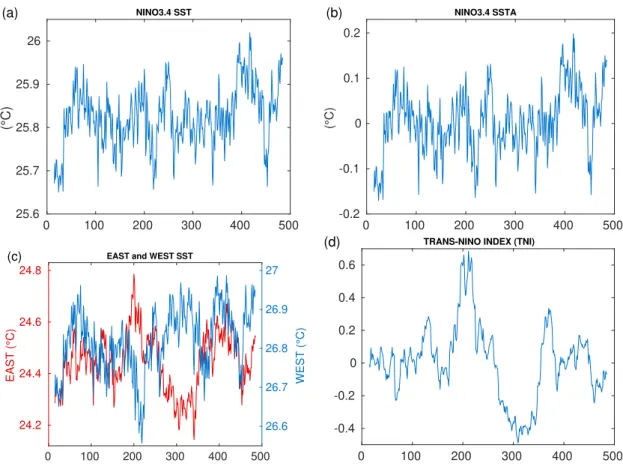
AlthoughtheNiño3.4indexisnotapableofdistinguishingbetweenthetwotypesofENSO
events, this will be ahievedbyombining itwith theTrans-Niño Index(TNI) (Trenberth and
Stepaniak, 2001). TNI aims to apture the spatially varying SSTA, separating the eastern
basin SSTA or EP events from the entral-western SSTA or CP events. The original index
omputes normalized Niño1.2 SSTA and subtrats the normalized Niño4 SSTA. Then, if the
largestanomalies arefound onthe east (west), TNIwill obtain positive (negative) values and
the ENSO event will be dened as EP (CP). Due to the GFDL-ESM2M model bias, whih
representsthe strongestSSTvariability anomalouslyawayfrom thesouthAmerianontinent
and therefore out of the Niño1.2 region, the mentioned index has to be modied (Equation
2.1). For our partiular study the eastern boxhave been shifted to 130
◦
W - 90
◦
Wand 5
◦
N -
5
◦
S,whilethewestern boxhasbeen transferred to 170
◦
E - 140
◦
W.
T N I = SST A E N − SST A W N
(2.1)SST A E N
andSST A W N
represent theeasternand western normalized SSTvariability,res- petively. ThestandardizationisahievedbysubtratingthemonthlySSTmeanofthe30yearrunningwindowand dividing itby thestandard deviationof thesame windowlength.
2.2.3 ENSO metris
For the ENSO representability, dierent metris have been applied and ompared to ERA-
20C.TheENSOasymmetry,thatis, the diereneinamplitudebetween El NiñoandLaNiña
events, isomputedastheskewnessofinterannualvariabilityofSST(BurgersandStephenson,
1999). After omputing the Niño3.4 SSTA, the skewness of the probability density funtion
willprovide us withinformation about theENSO asymmetry. In addition, to ndtheregions
of strongest ENSO asymmetry,the mentioned skewness hasbeen alulated for eah tropial
Pai spatialgrid point using theSSTAsand U10 anomalies (U10A) (Atwood et al.,2017).
TheseasonaldependeneontheSSTvariability,alsoalledtheENSOphaseloking,isthe
seondmetri. TheSSTvariabilityis inreasedduring themonthsofborealautumn, peaks in
winterandisonsiderablydereasedduringspring(RasmussonandCarpenter,1982). Toprove
the reliability of the GFDL-ESM2M's ENSO phase loking, we have omputed the standard
deviation of Niño3.4 SST for eah month. Nevertheless, in order to relate the seasonal SST
variability to other Niño regions, the study of the seasonality is also extended to the whole
equatorial(5
◦
N - 5
◦
S) Pai byusingtheHovmöller diagram.
The third metri orresponds to the spatial pattern of SST variability during the ENSO
events. ForthispurposewehaveomputedtheElNiñoandLaNiñaompositesandshowtheir
tropialPaiSSTApatterns. Independentlyanalyzingthem,weaninvestigateifthereisany
andtakingintoaount theENSOasymmetry,weaninvestigate theplausibleeetsonto the
mean tropial Pai state thattheresidual ofEl Niñoand La Niñaeventsould have.
TheENSOamplitudewasdetetedasinBellengeret al.(2014), alulatedasthestandard
deviation ofSST,butinouraseovertheNiño3.4region. Beauseourmaininterestisfoused
on the deadal variability of theENSO amplitude, a 30 year running standard deviation has
beenusedtoexposethelongtermvariability. InordertoomparethedeadalENSOamplitude
with ENSO event frequeny and EP - CP ENSO avors, the 500 year time series has been
split into 30 year bins, deteting the ENSO events with the above explained tehnique and
distinguishing the EP-CP events by the modied TNI index for eah binned period of time.
Finally, thesequene of El Niño - La Niña events is analyzed by applying theNiño and Niña
ompositeintheHovmöllerdiagrams,extendingthetimeevolutionofSSTAovertheequatorial
Pai 20monthsbefore andafter the month ofDeember.
2.2.4 Atmospheri feedbaks
ThemeanstateandvariabilityofthetropialPailimateisstronglydeterminedbyoupled
oean-atmospherefeedbaks(Lin,2007). Agenerilassiationofthosefeedbaksinthetropi-
al limate dividesthem,dependingon their positive or negative sign. Thetwo mostommon
feedbaks that onsider atmospheri proesses are the U10 feedbak and the NHFS feedbak
(Zebiak and Cane, 1987; Jin et al., 2006). With a positive sign, the U10 feedbak, or the
atmospheri omponent of the Bjerknes feedbak(Bjerknes, 1969), ismeasured asthedistant
zonal wind response to an anomalous SST over the entral-eastern equatorial Pai (Lloyd
et al., 2012). The anomalous westerly (easterly) wind anomalies ause a derease (inrease)
of thezonal SST gradient by attening(tilting) thethermoline slope. In return, the weake-
ning(strengthening) oftheSSTgradientfurtherdamps (exites)theeasterlywinds,forminga
positive feedbak. Similarly,a positiveSSTA overthe entral-eastern tropialPai swithes
ananomalousloalonvetionstateinsteadofaommonlyobservedsubsidene. Theonvetion
auseshigherpreipitation,whihinreasestheheatbylatentenergy,andloudoverandwater
vapor whih at as radiative heating. Hene, a positive feedbak is formed. Following Lloyd
et al. (2009) the U10 feedbak is omputed asa linear relation shown inEquation 2.2, where
τ x ′
representsthe U10A,beinga produt oftheSSTA (SST ′
)and theU10 feedbak(µ
).τ x ′ = µ × SST ′
(2.2)The main negative feedbak, the proess whih damps the anomalous SSTs, is the NHFS
feedbak. The SST anomalies are responded to by thermodynami hanges: positive SSTA
will ause an inrease of heatloss, mostly by latent uxes and the redutionof inoming SW
radiation bythe inreaseof CLT. Toa lesserextent,sensible uxand long-wave radiationalso
aet the exited SSTs (Lloyd et al., 2009). The NHFS feedbak omputation is visible in
the Equation 2.3. Similarly as in Equation 2.2, the negative feedbak (
α
) is obtained by therelationbetweentheNHFSanomalies(NHFSA)(
Q ′
)andSSTA.Followingthesameproedure,we have applied thesame equation to the two most dominant NHFS omponents: the LHFS
and theSWradiation (Lloyd et al.,2009, 2012).
Q ′ = α × SST ′
(2.3)First of all, the linear relation between thementioned variable anomalies and theNiño3.4
SSTAareomputed foreahtropialPaigridpoint. Onewehavedetetedtheregionwith
U10andNHFSsensitivities,itwillbeusedtoalulatethetemporalevolutionofthefeedbak.
Forinstane, the U10feedbakmaximumvaluesareloatedovertheNiño4area, whilefor the
NHFSfeedbakwewill ombine the Niño3and Niño4boxes.
2.2.5 Deadal ENSO amplitude modulation
Inorder to understand the possible auses and onsequenesof the deadal ENSO amplitude
variability, we have deteted and dierentiated between two time periods of high and low
ENSOamplitudes: theHighandLowepohs. Aftersettingbothperiodsto thesametemporal
length of 60 years, we have studied the mean state and variabilities of the tropial Pai
natural systemfor the SST, T, U10, W500,NHFS, PR and CLT. The interannual variability
hasbeen omputed asthestandard deviation, obtainingthe anomalies relative to the60 year
seasonal yle. Ogata et al. (2013) separated the studies relating the mean state and the
ENSOamplitude intotwo groups: the onesthatlookinto theENSOamplitude responsewhen
dierentstohastiforingareappliedtomultiple meanstates,andtheseondonesexamining
theinteration between themean stateand theENSO amplitude.
Ourresearh would tinto the seond study-type: besidesthemeanstate and interannual
variability, we have alulated the whole ENSO harateristis and linear atmospheri feed-
baks for both epohs. Thiswill help us understand thepossible eets ofthe ENSOmetris
dierenes,like its amplitude,asymmetryand spatialpattern onto themeanstate.
Furthermore, the possible auses for the ENSO deadal variability are investigated. A li-
near Pearson orrelation has been used to study the relation between the ENSO amplitude,
atmospherifeedbaks andthe mean state.
Following Bellenger et al. (2014), our last but not the least important fous is set on the
non-linearexpressionsoftheGFDL-ESM2Moupledlimatemodelfeedbaks. Ourintentionis
toobtainfurtherinformationaboutthepossibleausesforthedeadalENSOamplitudemodu-
lation. We have split the months between positive and negative Niño3.4 SSTA, for both the
HighandLowepohs, andthen obtainseparatelinear relationships withU10Ato understand
thewind sensitivityto surfaetemperature anomalies.
Similarly,we have applied the SWanomalies (SWA)into our non-linear analysis, whih is
known to be the main soure of ENSO error within limate models (Kim and Jin,2011). In
observations,the SWfeedbakisaptured asapositivefeedbak,whenSSTAsobtainnegative
values. In a subsideneregime, aSST inrease will ause adestabilization of theatmospheri
boundarylayer,restriting the stratiformloudformation, inreasing theSWradiationand in
turninrease the SST. Onthe ontrary,when the SSTAsare positive, thatis, in aonvetive
regime, the SW feedbak is turned negative. In this ase an inrease of SST will produe an
inrement of CLT, aderease of theinoming SWradiation and a redution ofthe perturbed
SST(Philanderetal.,1996;Xie,2004). Fromthisanalysiswewillretaininformationaboutthe
abilityofthemodelto demonstrate the system'sshift between onvetive/subsidene regimes.
The nextnon-linear variability showninour researhis relatedto W500anomalies, whih
infatwill provide furtherinformation abouttheabilityofthesystemtoshiftfromsubsidene
the Niño3 box, adomain inwhih the vertial windvariability diersthemost andstrong EP
eventsourduringtheHighepoh. Hene,the non-linearanalysisinthisasewillinvolve the
Niño3 area.
Thelastpossiblenon-linearrelationwiththedeadalENSOamplitudehasbeenattributed
to the mean thermoline slope. The thermoline depth is omputed asthe strongest vertial
temperature gradient instead of the ommonly used 20
◦
C isotherm. The seond mentioned
approahofthethermolineisnotreommendedunderlong-termmeanstatehanges(Yangand
Wang,2009). SimilarlyasinHuet al.(2013),whodemonstrated thatatoolargeor tooweak
thermolinetiltdereasestheENSOamplitudeformingaonavefuntion,thethermolinetilt
isalulated bythe dierene ofthemeanthermoline depthbetweentheeasternandwestern
equatorial Pai. The western box is set to 160
◦
E - 170
◦
W, 5
◦
N - 5
◦
S and theeastern area
to 120
◦
W - 90
◦
W, 5
◦
N - 5
◦
S.In order to represent the deadal relationship, we have applied
a 30 yearrunning meanto the monthly thermoline tiltdata.
Results
3.1 ENSO simulation skills
The GFDL-ESM2M model is known to reprodue relatively realisti ENSO dynamis and it
hasbeenhosenasoneofthebestoupledlimatemodeloptionwithintheCMIP5group(Kim
andJin,2011;Bellenger etal.,2014;Kimetal.,2014;Capotondietal.,2015). Furthermore,its
strongatmospheri feedbaks have been foundto be relativelylose tothe observations (Bayr
et al., 2019). In the rst hapter we will analyze some of the harateristis of the present
limatemodel, omparingitto theERA-20Creanalysis produt,starting fromthemeanstate
model bias and ontinuing with the relevant ENSO statistis and feedbaks. Both the mean
stateandfeedbaksareimportantfatorstoobtaingoodENSOdynamis,asithasbeenproven
inmanypreviousstudies(KimandJin,2011;Lloydet al.,2012;Hametal.,2013;Dommenget
et al., 2014). Therefore, this setion will be of great importane in order to understand the
behaviorof thesimulation obtained withthe GFDL-ESM2M limatemodel.
3.1.1 Model bias in the mean state
Many limate models have relevant issues when simulating the realisti representation of the
tropial Pai mean state. One example is the old SST bias over the equatorial region.
Theold tongue bias,as thenegative bias inthe mean state is alled, simulatesa ontinuous
La Niña-like state: the old SST over the equatorial Pai leads to an intensiation of the
easterlieswestoftheNiño4region,pushingthewesternPaionvetiveregionwestward,and
henedisplaingthe risingbranhoftheWalkerCirulation. Iftherisingbranhisloatedtoo
farwest,theonvetiveresponseisgreatlydereasedandthereforethestrengthoftheU10and
NHFSfeedbaksisredued, ausing dierent ENSOdynamis (Daveyetal., 2002;Bayr etal.,
2018).
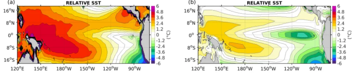
The hosen modelfor this researhis not an exeption. Figure3.1 demonstratesthe die-
renesintherepresentation ofthemeantropialPaiSST.Inordertomaketheomparison
easier,insteadof the absolutetemperatures, we showthe meanSSTrelative to theareamean
of the tropial Pai (120
◦
E-80
◦
W, 20
◦
N-20
◦
S). In addition, the distribution of the relative
SSThasalargerimpatonthetropialatmospheriirulationthantheabsolutevalues(Bayr
andDommenget,2013).
Althoughthe general pattern oftherelativeSSTissimilar toERA-20Creanalysis produt
with warmtemperatureson the west andold ontheeast,thegradient or thetransitionfrom
positive to negative relative SST is shifted 60
◦
to the west, onning the Pai Warm Pool
to the very western equatorial region, and displaing the minimum SST values away from
the South Amerian oast. Furthermore, the SST dierene between the GFDL-ESM2M and
ERA-20C(Figure 3.2a) demonstrate anegative equatorialSSTbias above 1
◦
C, andapositive
bias above 3
◦
C along the South Amerian oastline. Due to the old bias the atmospheri
irulation shows an anomalouspattern: strongereasterlies over theNiño4 region andwest of
Central Ameria are found, while o the oast of Peru weaker mean zonal winds are visible
(Figure 3.2b).
Figure 3.1: Themeanseasurfaetemperature(SST)relativetotheareameantropialPaiSST
for: a)ERA-20C, andb)GFDL-ESM2M.
Figure 3.2: Meanstatemodelbiasfora)theseasurfaetemperature(SST),andb)thesurfae
zonal winds(U10),obtainedbythedierenebetweentheGFDL-ESM2M modelandtheERA-20C
reanalysisprodut.
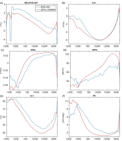
Figure 3.3 represents the zonal equatorial struture (5
◦
N-5
◦
S) of the relative SST, U10,
W500, NHFS,CLT, and PR. The mentioned old bias strengthens the easterlywinds west of
150
◦
W, pushing the rising branh of the Walker Cirulation 15
◦
to the west. In addition, the
rising branh of the Walker Cirulation auses too high CLT and PR and too weak NHFS,
while on theeasternside thetoo strong subsidene state shownbythedownward windsleads
to lessCLTand PRwitha strongerNHFS whenomparing to ERA-20C.
Hene,duetotheequatorialoldbiasandaonstantLaNiña-likestate,therisingbranhof
the WalkerCirulation isloatedfar too westand thesubsidene stateis anomalouslystrong,
extending slightly west ofthedate line.
120E 150E 180 150W 120W 90W -4
-2 0 2 4
(°C)
RELATIVE SST ERA-20C GFDL-ESM2M
(a)
120E 150E 180 150W 120W 90W -6
-4 -2 0 2
(m/s)
(b) U10
120E 150E 180 150W 120W 90W -0.06
-0.04 -0.02 0 0.02
(Pa/s)
(c) W500
120E 150E 180 150W 120W 90W 30
60 90 120
(W/m²)
(d) NHFS
120E 150E 180 150W 120W 90W 40
50 60 70 80
(%)
(e) CLT
120E 150E 180 150W 120W 90W 2
4 6 8 10
(mm/day)
(f) PR
Figure3.3: EquatorialPaimeanstate(5
◦
N-5
◦
S)ofa)seasurfaetemperature(SST),b)surfae
zonalwinds (U10),)vertialwindat500hPaheight(W500),d)netheatux(NHFS),e) totalloud
over(CLT)andf)preipitation(PR).GFDL-ESM2Min redandERA-20Cinblue.
3.1.2 ENSO metris
In the present subsetion we will pay attention to the ability of the GFDL-ESM2M limate
modelto reprodue multiple ENSOharateristis.
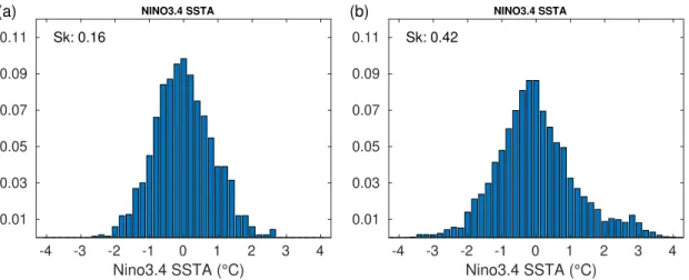
First of all we must highlight its strong non-linear behavior when simulating the ENSO
events, as presented by the probability density funtion (PDF) of Niño3.4 sea surfae tem-
perature anomalies (SSTA) (Figure 3.4). In both ases, ERA-20C and GFDL-ESM2M, the
distributionhas apositive skewness: the tail ofthe PDFis elongatedtowardspositive values,
representingstrongerpositiveSSTAthannegativeones. However,thelimatemodel'sskewness
is about three times larger than that of ERA-20C, 0.42 and 0.16 respetively, revealing that
theGFDL-ESM2M modelhasrelatively strongerEl Niñothan La Niñaevents.
NINO3.4 SSTA
Sk: 0.16
-4 -3 -2 -1 0 1 2 3 4
Nino3.4 SSTA (°C) 0.01
0.03 0.05 0.07 0.09 0.11
(a) NINO3.4 SSTA
Sk: 0.42
-4 -3 -2 -1 0 1 2 3 4
Nino3.4 SSTA (°C) 0.01
0.03 0.05 0.07 0.09 0.11 (b)
Figure 3.4: Probabilitydensityfuntion ofNiño3.4seasurfaetemperatureanomalies(SSTA).The
skewnessvalue,representingtheENSOasymmetry,isdisplayedintheupperleftornerof theplots:
a) ERA-20C,andb)GFDL-ESM2M.
The geographial distribution of the tropial Pai SSTA skewness (Figure 3.5) also dis-
plays relevant dierenes. Both the map for ERA-20C and GFDL-ESM2M show a dipole
pattern: positive skewness on the east equatorial Pai resembles stronger positive SSTAs
than negative, that is, stronger El Niño than La Niña events. However, when El Niño is de-
veloping,theoeani heatontent isdisplaedfromthe western equatorialPaitowards the
east, and hene, negative SSTAs areloatedoverthe edge ofthe Pai WarmPool: positive
skewness in the east is related to negative skewness in the west. It must be said that both
representations agree on the loation of the highest skewness: the strongest asymmetries are
situated on the easternPai, theloationof thesoalled EP El Niñoevents.
Figure 3.5: SkewnessmapoftropialPaiseasurfaetemperatureanomalies(SSTA)fora)
ERA-20C, andb)GFDL-ESM2M.
Nevertheless,theextensionofthementionedpositiveskewnessisexaggeratedintotwomain
regions(south andnortheastequatorialregions)andthenegative skewnessis displaedfartoo
the west, agreeingwith the loation of the Pai Warm Poolbeing too far west. Beause of
the old equatorialbiasandstrong western equatorial U10,theedgeof thePai WarmPool
is limited to the west, allowing the strong positive SSTA to spread further west and limiting
the eastward extension of the negative skewness in the limate model. In addition, both the
Figure3.6: SkewnessmapoftropialPaisurfaezonal windanomalies(U10A)fora)ERA-20C,
andb)GFDL-ESM2M.
Similarly, the skewness of U10A (Figure 3.6) is positioned far too the west ompared to
ERA-20Candthestrongervaluesillustratethehighlynon-linearbehavioroftheGFDL-ESM2M
oupledmodel onemore.
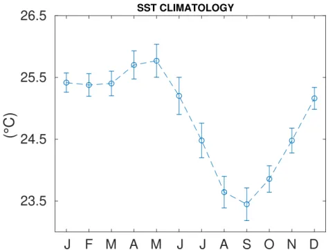
AnotherimportantENSOharateristiisitsphaseloking. ThehighestNiño3.4SSTstan-
darddeviationistwomonthsdelayedforthethelimatemodel(Figures3.7a,b,). Nevertheless,
themodelisapable ofreproduing thehighestNiño3.4SSTstandard deviationduringboreal
wintermonthsalongwiththedampingofitsvariabilityduringspring. Thisisarelatively lose
approximation to realisti ENSO dynamis, in whih ENSO grows during autumn, peaks in
thewinter months and isdamped duringspring (Rasmusson andCarpenter,1982). A seond
smallerpeakofthestandarddeviationisvisibleduringthemonthofJuly. Theanomalousdou-
blepeakof SST variability is due to the double(semiannual) ITCZ and the seasonal reversal
ofthemeridionalSSTgradientand windsinthe east(Wittenberg etal.,2006). TheHovmöller
diagramoflatitudinallyaveraged(5
◦
N-5
◦
S)SSTvariabilityrepresentsthementionedbehavior:
both peaks are equally strong, but during boreal summer months the variability is extended
furtherwest, apturing itbythe Niño3.4regionwithhigher magnitude (Figure3.7).
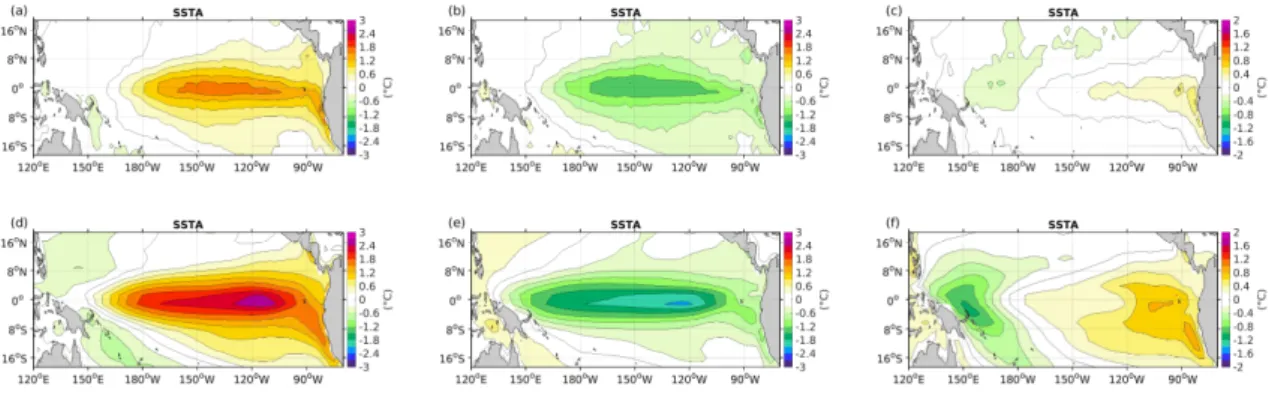
Thegeographial position oftheSSTA usingEl Niño and LaNiña omposites isvisible in
Figure3.8. Asshown before, both the positive and negative SSTA extend too far west in the
present limatemodeland itsintensityisgreatly enhanedwhenomparingto ERA-20C.The
largestpositive SSTA isloatedat 120
◦
Wandthenegative SSTA isslightly shiftedwestward.
Thereanalysis produt, on the other hand, hasboth a positive and negative SSTA maximum
entered in the equatorial Pai setion. The dierene between the eets of El Niño and
La Niña events, that is, their residual, is demonstrated by adding both omposites. El Niño
events tendto warmthe very easternsetion, whileLa Niñasaet more stronglythewestern
region. The result is a dipole pattern for both the limate model and the reanalysis produt.
Thedierenesarevisibleinthemagnitudeandthe loation: thelimatemodelhasastronger
dipolepattern withthe negative valuesloatedtoofar west.
Although theGFDL-ESM2M isknownfor itsrelatively realisti ENSOdynamis,itseems
that it has diulties to reprodue proper ENSO harateristis: the ENSO asymmetry is
anomalously large, the phase loking is delayed, it shows a double SSTA standard deviation
peak, andLaNiñaandElNiñoeventstendto extendtoofarwestalongtheequatorialPai.
Inaddition, thepresent limate modeldoesn't seem to reprodue realisti EPEl Niño events,
J F M A M J J A S O N D 0.6
0.7 0.8 0.9 1
ERA-20C (°C)
0.9 1 1.1 1.2 1.3
GFDL-ESM2M (°C)
NINO3.4 SST STD
(a)
SST STD
120°E 150°E 180° 150°W 120°W 90°W Jul
Aug Sep Oct Nov Dec Jan Feb Mar Apr May
Jun 0.25
0.5 0.75 1 1.25 1.5 1.75
(°C)
(b) SST STD
120°E 150°E 180° 150°W 120°W 90°W Jul
Aug Sep Oct Nov Dec Jan Feb Mar Apr May
Jun 0.25
0.5 0.75 1 1.25 1.5 1.75
(°C)
(c)
Figure 3.7: Monthlystandarddeviationoftheseasurfaetemperatures(SST)over: a)theNiño3.4
region, ERA-20CinblueandGFDL-ESM2M modelin red,b)thePaiequatorial(5
◦
N-5
◦
S)region
forERA-20C,and )thesameasb)butforGFDL-ESM2M.
Figure 3.8: GeographialloationofERA-20CreanalysisproduttropialPaiseasurfae
temperatureanomalies(SSTA)froma)ElNiñoomposite,b)LaNiñaomposite,and)theirresidual
obtainedbyaddingbothomposites. Similarly,d)e) andf)orrespondto theGFDL-ESM2M model.
3.1.3 Atmospheri feedbaks
The atmospheri positive and negative feedbaks are of great importane for induing ENSO
growth and damping, respetively. Hene, their orret simulation will ause a substantial
improvement on the ENSO properties suh as El Niño/La Niña asymmetry or phase loking
(Bayretal.,2018). Bayretal.(2018)statethedependeneoftheSSTmeanstateonsimulating
the ENSO atmospheri feedbaks. They onluded that the U10 and NHFS feedbaks at
linearly depending on the equatorial SST mean state, ompensating eah other's biases, but
leading toerroneous ENSOproperties.
Thewindisknowntoatasapositivefeedbak: thepositiveSSTAovertheNiño3.4region
dereasesthezonal SSTgradient overtheequatorialPai, andhenethezonalwindson the
easternequatorialregion andthe thermoline tiltareredued, induing a furtherheating: the
Bjerknes feedbak (Bjerknes, 1969). In ontrast, the NHFS ats to redue the oeani heat
ontent when SSTA inreases. LHFS and SW radiation are the dominant variables aeting
theNHFS (Lloyd etal.,2009). For instane,when positive SSTA areloatedovertheNiño3.4
region, higher evaporation releases a larger amount of heat energy, inreasing the LHFS. In-
reasing the loud over over the anomalous SST region redues the inoming SW radiation
towardsthe surfae ofthe oeanbyreeting itbak: thealbedo eet. Thereforeit isonsi-
deredto be anegative feedbak,whih playsamajorrolein damping ENSOevents duringthe
monthsofspring (Dommenget andYu,2016;Wengel etal., 2017).
Applying a simple polynomial t of the rst order, we get a linear regression that relates
U10andNFHSanomaliestoNiño3.4SSTA.Theslopeofthepolynomialtwillbethestrength
ofthefeedbak.
Therststepforthefeedbakanalysisistodetet theregionsinwhihtheU10andNHFS
areaetedthemost bythe Niño3.4SSTA. Therefore,wewill ompute thefeedbaksfor eah
spatialgridpoint alongthetropial Pai,relatingU10Aand NHFSA to Niño3.4SSTA.
Figure3.9: Linearwind(U10)feedbak: anomaloussurfaezonalwind (U10A)sensitivityto
Niño3.4seasurfaetemperatureanomalies(SSTA)foreahtropialPaigridpointfora)
ERA-20C,andb)GFDL-ESM2M.
Figure3.9shows thelinearrelationshipbetween theNiño3.4SSTAand U10A.Inthis ase,
we must say thatthe U10 feedbak simulation is very similar to the reanalysis produt, both
in strength and loation. For the GFDL-ESM2M model however, the positive feedbak still
◦
both ases agreethat thestrongest U10 feedbak isloated lose totheNiño4 region.
Figure 3.10: Linearnetheatux(NHFS)feedbak: anomalousnetheatux (NHFSA)sensitivityto
Niño3.4 seasurfaetemperatureanomalies(SSTA)foreah tropialPaigridpointfora)
ERA-20C, andb)GFDL-ESM2M
The main negative feedbak, theNHFS feedbak, is spread over a larger equatorial region
(Figure3.10). ThelimatemodelshowssubstantialdiereneswhenomparingittoERA-20C:
it is weaker in magnitude and its maximum is separated in two main domains, one entered
at 120
◦
W and the other one at 180
◦
. The ombination of Niño3 and Niño4 regions will be
onsidered asthe loation of the strongest relationship between theNHFSA and the Niño3.4
SSTA.
J F M A M J J A S O N D 0.6
0.9 1.2 1.5
(m/s per °C)
-20 -15 -10 -5 0
(W/m² per °C)
MONTHLY FEEDBACK
U10 NHFS LHFS SW
Figure 3.11: Monthlywind(U10)feedbakin redandnetheatux (NHFS)feedbakinsolidblue.
Thenetheatux feedbakhasbeendividedinto latentheat ux(LHFS)shownasdashedblueand
shortwaveradiation(SW)asdash-dotblue. Niño3.4seasurfaetemperatureanomalies(SSTA)have
beenlinearlyrelatedtoNiño4surfaezonalwind anomalies,andwiththeombinationofNiño3and
The seasonality of the feedbaks an be observed in Figure 3.11. The U10 feedbak has
strongestvalues from Otober to Deember, theseason inwhih theSST varies themost and
theENSOevents grow. However, a seondpeakis visibleduring May,whihould berelated
tothedoubleITCZandrelaxationoftheeasterlies,heneformingaseondpeakontheENSO
phase loking (Figure 3.7a). The NHFS, as demonstrated by Lloyd et al. (2009), is mostly
governedbyLHFSandSWfeedbaks. ItpeaksfromJanuarytoApril,reduing thevariability
oftheNiño3.4SSTand leading to relatively realisti ENSOphaseloking.
From our feedbak analysis we ould argue that the GFDL-ESM2M limate model has a
quiterealistirepresentation of the U10feedbak,although itextendstoo farinto thewestern
equatorialPai. However, themodelshowslarger deienies when simulating thenegative
NHFS feedbak: its maximum values are split into two equatorial domains and the absolute
values areoverallweakerthaninERA-20C.Hene, sinetheSSTvariabilityisover-exitedby
thepositivefeedbak, mostlyinthewesternequatorialPai,butitistooweaklydampedby
theNHFS feedbak, exessively ative ENSOeventsareto beexpeted.