Institut für Höhere Studien (IHS), Wien Institute for Advanced Studies, Vienna

(1)

Reihe Transformationsökonomie / Transition Economics Series No. 6

Estimation of Income, Own- and Cross-Price Elasticities

An Application for Bulgaria

Emil Stavrev, Gueorgui Kambourov

(2)

Estimation of Income, Own- and Cross- Price Elasticities

An Application for Bulgaria

Emil Stavrev, Gueorgui Kambourov

Reihe Transformationsökonomie / Transition Economics Series^*) No. 6

*) Die Reihe Transformationsökonomie ersetzt die Reihe Osteuropa.

The Transition Economics Series is a continuation of the East European Series.

March 1999

Emil Stavrev

Institute for Advanced Studies Department of Economics

Stumpergasse 56, A -1060 Vienna, AUSTRIA Fax: ++43/1/599 91-163

E-mail: stavrev@ihs.ac.at and

CERGE-EI

Politických V•zÁu 7, CZ-111 21 Prague 1 CZECH REPUBLIC

E-mail: emil.stavrev@cerge.cuni.cz

Gueorgui Kambourov CERGE-EI

Politických V•zÁu 7, CZ-111 21 Prague 1 CZECH REPUBLIC

and

UWO, CANADA

E-mail: gkambour@julian.uwo.ca

Institut für Höhere Studien (IHS), Wien Institute for Advanced Studies, Vienna

(3)

The Institute for Advanced Studies in Vienna is an independent center of postgraduate training and research in the social sciences. The publication of working papers does not imply a transfer of copyright. The authors are fully responsible for the content.

(4)

Abstract

In this paper we estimate income elasticities and own- and cross-price elasticities for a number of categories of goods. The methodology used was proposed by Deaton (1987). Expenditure and quantity data from Household Budget Surveys for Bulgaria are used. The households are geographically separated into clusters. The prices are assumed to be the same within each of the clusters, so that the effects of income and other demographic factors on unit values are determined and the variances and covariances of the measurement errors estimated in the first stage. Then, in the second stage, the spatial price variation between the different clusters is used for the estimation of own- and cross-price elasticities for various categories of goods. We report income elasticities and own- and cross-price elasticities for eight goods.

Keywords

Own- and cross-price elasticities, income elasticities, unit values, quality effects

JEL Classifications

C39, C51, D12, R22

(5)

Comments

This research was undertaken with support from the European Union's Phare ACE Programme 1996 (Gueorgui Kambourov P96-6701-F and Emil Stavrev P96-7156-S). We would like to thank Prof.

Lester D. Taylor, Prof. Andreas Wörgötter, and our colleagues at the Center for Economic Research and Graduate Education in Prague and the Institute for Advanced Studies in Vienna for many helpful comments. All errors, however, are ours.

(6)

Contents

1. Introduction 1

2. Theoretical Background 2 3. Econometric Estimation 5 4. The Data 7

5. Results 9

5.1. First Stage 9 5.2. Second Stage 10

5.3. The Dynamics of Income, Own- and Cross-Price Elasticities in 1992 and 1993 14

5.3.1. Income and Quality Elasticities 14 5.3.2. Own- and Cross-Price Elasticities 15

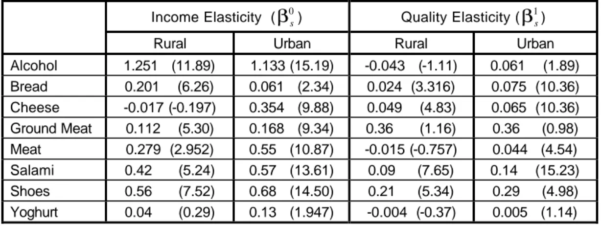
5.4. Comparing Urban and Rural Income, Own- and Cross-Price Elasticities for the Year of 1993 16

5.4.1. Income and Quality Elasticities 16 5.4.2. Own- and Cross-Price Elasticities 17

6. Conclusion 19 References 20

(7)

1. Introduction

Given the easy comprehensibility and enormous importance for policy-makers of the elasticity concept, the estimation of elasticities has been one of the main trends in applied demand analysis. Since the 1930s (see Allen and Bowley [1935], Bergson [1936], De Wolff [1938], and Schultz [1938]), economists have been constantly improving their methodologies and model specifications in order to extract information on different elasticities from cross-sectional and time-series data.¹ For the estimation of price elasticities, time-series data seemed to be the most useful, and it was deemed quite unfortunate that most of the developing countries lacked such data. Deaton (1987, 1988, 1990), however, introduced a procedure which enables researchers to estimate own- and cross-price elasticities from household budget surveys.

Since such surveys are available for a large number of developing countries, this new approach has an enormous practical application.

Most of the countries in transition do not have a long enough record of time-series data to allow the estimation of the price elasticities of certain goods. Nevertheless, for the conduct of a wise fiscal policy  especially during the period when the economy is being restructured  governments need to know the approximate magnitude of the elasticities of some important goods. It is also true that the ex-socialist countries used to gather reliable and sophisticated household budget surveys. Therefore, it is of great interest to determine whether and how the proposed methodology could be applied to countries in transition.

The household budget surveys contain data on expenditures and purchased quantities.

Therefore, one could derive proxies for the goods’ prices  their unit values  by dividing the expenditures on a given good by the quantity purchased. However, “goods” usually represent an aggregation of commodities, so that cheese, for example, would contain white cheese, yellow cheese and other kinds of cheese. What is more, we may have different qualities of each of these. This presents a number of problems. First, an increase in household income would most likely increase the unit values, since richer households would tend to buy higher quality goods. Second, quality itself is determined by the price of cheese and all other relevant goods. Finally, a measurement error is likely to exist due to the fact that both expenditures and quantities are measured with error.

The central idea in Deaton’s analysis is to divide the households geographically into clusters.

The prices are assumed to be the same within each of the clusters, so that the effects of income and other demographic factors on unit values can be determined and the variance- covariance matrix of the measurement error estimated. Then, in the second stage, the spatial price variation between the different clusters is used for the estimation of own- and cross-price elasticities for various categories of goods.

1 An excellent survey of the initial fundamental works in this field is given by Brown and Deaton (1992), “Surveys in Applied Economics: Models of Consumer Behaviour”, Economics Journal, 82, 1145−^1236.

(8)

The paper is organised as follows: in Section 2, the theoretical background of the model is described; in Section 3, we discuss the estimation procedure and the various econometric considerations; the data used and the way it was processed is discussed in Section 4;

Section 5 presents the results that we obtained, while Section 6 concludes the discussion.

2. Theoretical Background

The data we have are on composite goods such as meat, yoghurt, and salami. Each of these categories contains different goods which are themselves of different levels of quality. The households which participated in the surveys recorded both quantities and expenditures.

Therefore, in the data we find, for example, that a certain household for a certain period of time spent 1000 leva buying 20 kilograms of cheese. Dividing the former by the latter  which would be the unit value of cheese  could be used as an indicator that the price of cheese is 50 leva per kilo. It is then straightforward to derive the own- and cross-price elasticities by running a regression of the quantity purchased on the unit value, income, and several other characteristics.

There are, however, a number of problems with such an approach. Prais and Houthakker (1955) noted that unit values seem to be positively correlated with household income. Quality choice also depends on prices since a change in the price of cheese or any other relevant good might have an influence on the quality of cheese consumed by the households. As a result, the price changes would be different from the unit value changes corresponding to the same changes in the quantity consumed. Therefore, the price elasticities might be exaggerated.

Since, most probably, expenditures and quantities have been measured with errors, measured unit values are likely to be negatively correlated with measured quantities.

The above discussion could be analytically presented as follows. Let p_s be the vector of prices in the group S. The households are divided geographically into different clusters c. The expenditure on one group is E_s = p x_s^' _s^{, where x}s is the vector of consumed quantities.

p_s = ν_sp_s^*, (1)

where, νs is defined as a scalar (Paasche) linear homogenous price level for the group (for example, the price of milk relative to the other goods), and p_s^* is deemed as the “fixed price structure” of the relative prices in group S, assumed to be the same for all clusters.

The difference among the prices in different clusters is brought by νs. A group quantity index Xs is defined as

(9)

X_s =(n_s⁰)^'x_s, (2)

where, n_s⁰ is a vector of ones (and then (n_s⁰)^'x_sis simply kilograms or liters) or anything else that might be deemed important (as calories).

The unit value, µs, is

µ_s ^s ν

s s

E X

p x n x

= = ( )

( )

* ' '

0 . (3)

From here

lnµ_s =lnν_s +lnq_s, (4)

where, qs equals ( ) ( )

* ' '

p x n x

s s

0 and stands for quality. If better-off households purchase bundles that contain a larger share of high price per kilo items then µ_s will rise with income. The income elasticity of µ_s was defined by Prais and Houthakker as “quality elasticity” (see equation 9 below).

The specified utility function is

^u ⁼ ^{f u x}

[

¹

( ) ( )

¹ ^,^{u x}² ² ^{,. ..,}^{u x}^s

( )

^s ^{, ... ,}^u^m

( )

^x^m

]

^, ⁽⁵⁾

where each of the goods form a separable branch of preferences. From this it follows that the demand function for each good is

^x^s ^{x E p}^s

(

^s ^s

)

^x^s ^E^s ^p

s

= =  s

 



, , ^*

ν ^. ⁽⁶⁾

Then,

∂

∂ ν

∂

∂ δ ∂

∂ ν ln

ln

ln ln

q q

E

s E

z

s s

sz

s z

= −  −

 

^, ⁽⁷⁾

where δsz is the Kronecker delta, and

(10)

∂

∂ ν δ ∂

∂ ν ε ln

ln

ln ln

E_s q

z sz

s z

= + + sz, (8)

where εsz is the cross- or own-price derivative of S with respect to Z.

Prais and Houthakker defined their quality elasticity as

ζ ∂

∂

s

qs

= lnm

ln ^, ⁽⁹⁾

where m is total expenditure (or income).

Thus,

( )

∂

∂ ζ ε

ln ln

ln ln q

m

q E

E m

q E

s s

s

s s

s

s s

= ⋅ = + ^, ⁽¹⁰⁾

where εs is the total income elasticity of the purchased quantity X_s. Using (7), (8), and (10), we get

∂

∂ ν

ε ∂

∂

ε ζ ε ln

ln

ln ln ln ln q

q E q E

s z

sz

s s s s

sz s s

=

−

= 1

,

(11)

and finally

∂ µ

∂ ν δ ζ ε ε ln

ln

s z

sz

s sz s

= + . (12)

Equation (12) gives us the desired relationship between price changes and unit value changes.

If there is no significant quality elasticity (ζ_s = 0), then the unit value would change as much as the price changes. In general, ζ_s would be greater than zero since richer households are expected to consume higher quality goods. Total income elasticity of the purchased quantity,

(11)

ε_s, is also expected to be positive since we are dealing with normal goods. Therefore, the unit value would tend to increase less than the price and, as a result, the price elasticity would be overestimated.

3. Econometric Estimation

We can postulate two regression equations for each of the goods that we consider in our demand system: the quantity equation and the unit value equation. The quantity demanded and the unit value of the goods in group S consumed by household i, which is in cluster c, is

( )

lnx_S _s _slnm_ic ( _s)^'G_ic _sz lnp f u

z

zc S G

ic = + + + + c + ic

∑

=

α⁰ β⁰ γ⁰ θ

1 8

0 , (13)

lnµ_s α_s β_sln _ic (γ_s)^' _ic ψ_szln _zc

z

m G p uS

= + + + + ic

∑

=

1 1 1

1 8

1 . (14)

Equation (13) is a double-logarithmic demand function. mic is total household expenditures per household member, and Gic is a vector of demographic characteristics for household i in cluster c. f_S

c is a cluster-specific fixed effect, while u_G

ic

⁺

(

û^S¹îc ⁻û^{S c}¹^⋅

)

^.

(16)

The notation “.” indicates means over all households in cluster c. For example lnx_{S c}_⋅ denotes the mean of the logarithm of the quantity of good S in cluster c. From (15) and (16) we can

(12)

estimate the income elasticities (β⁰_s) and the quality elasticities (β¹_s). The residuals are used for the estimation of the variances and covariances of the measurement errors.

The estimated β~⁰_s , β~¹_s , γ~_s⁰ and γ~¹_s are further used in the second stage of estimation. Let us define

~ ln ~

ln ~

y_{S c}_⋅ = x_{S c}_⋅ −β_s⁰ m_⋅_c −γ_s⁰G1_⋅_c and (17)

~ ln ~

ln ~

w_{S c}_⋅ = µ_{S c}_⋅ −β_s¹ m_⋅_c −γ_s¹G1_⋅_c. (18)

From here we derive the population counterparts

( )

y_{S c} _s _sz p_zc f u

z

S_c S c

⋅

= ⋅

=^α⁰ +

∑

^θ + +

1 8

ln 0 and (19)

w_{S c} _s _sz p_zc u

z

⋅ S c

= ⋅

=^α¹ +

∑

^ψ +

^u^Sic¹ ^,^u^Zic⁰

)

⁼^σ¹⁰^sz^, ⁽²⁴⁾

where σsz

10 and σsz

11 are the population moments.²

We can estimate,

2 ^σ^sz^rt

( )

^S^r ^Z^t

i c

n C k e e

ic ic

= − − ⁻¹

∑ ∑

, r, s = 0,1 and S, Z = 1,8

where r = 0 for the quantity equation and r = 1 for the unit value equation.

(13)

( ) ⁽ ⁾

~ ~ ~ ~ ~

Β= S −ρ⁻¹Ω ⁻¹ R−ρ⁻¹Γ ^, ⁽²⁵⁾

( )

p

c

limΒ~ Ψ' Θ'

→∞

= −¹ , (26)

where ρ⁻¹ =^C⁻¹

∑

ⁿ^c⁻¹ is the “average” cluster size.

Noting from (12) that

Ψ = +I DΘ, (27)

where D is a diagonal matrix with d_sz ^sz ^s

s

= δ β β

1

0 , we derive

( )

~ ~ ~' ~'

Θ= −I ΒD ⁻¹Β, (28)

which is a consistent estimator of the matrix of own- and cross-price elasticities.³

4. The Data

The data are from the 1992 and 1993 Household Budget Survey for Bulgaria for approximately 2500 households.⁴ We have the values and quantities for the following nine groups of goods:

alcohol, bread, cheese, ground meat, meat, salami, yoghurt, shoes and electricity. These categories, however, are aggregated goods, and therefore (1) alcohol includes beer, fruit wines, grapes wines, liquors, hard liquors (rum, vodka, brandy, whiskey, cognac, etc.), and rakiya⁵; (2) bread includes more than ten types of bread and a large variety of bakery products; (3) cheese includes white cheese (sheep, cow, mixed), yellow cheese (spread cheese, smoked cheese, and special brands), sour cream, and ice-cream (all brands); (4) ground meat includes various types of ground meat, (5) meat includes all types of meat; (6) salami includes various types of salami; (7) yoghurt includes all types of yoghurts; and (8) shoes includes all types of men’s shoes, women’s shoes, and children’s shoes.

3 For derivation of the variance-covariance of the~

Θmatrix, see Deaton (1987).

4 Having only the household code, we were not able to find out whether the same sample of households was used in both surveys.

5 A traditional Bulgarian brandy.

(14)

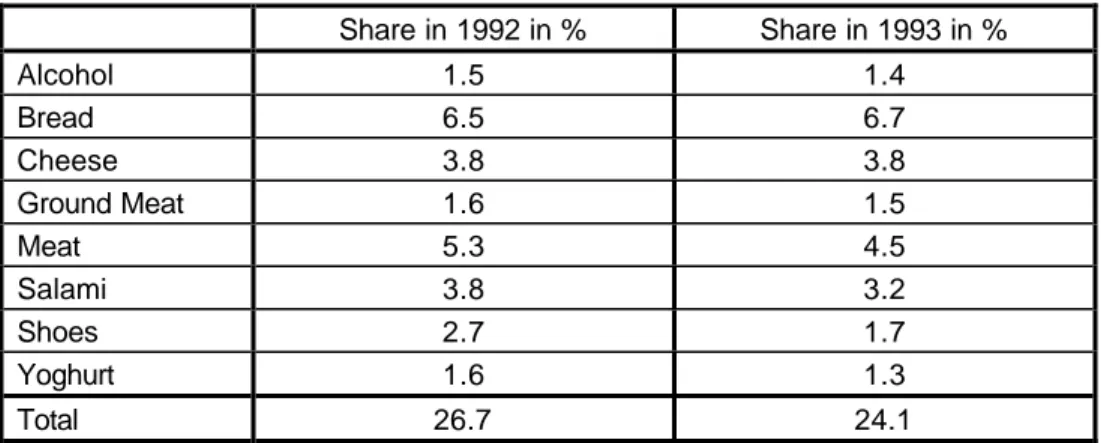
In table 1 below we give the average shares of the different goods in the total expenditure of the households, as well as the share of the whole system of goods in the total expenditure for the years 1992 and 1993.

Table 1: Shares of the goods in total expenditure

Share in 1992 in % Share in 1993 in %

Alcohol 1.5 1.4

Bread 6.5 6.7

Cheese 3.8 3.8

Ground Meat 1.6 1.5

Meat 5.3 4.5

Salami 3.8 3.2

Shoes 2.7 1.7

Yoghurt 1.6 1.3

Total 26.7 24.1

We have divided the households geographically into clusters. First, the separation was done according to the 28 districts into which Bulgaria was divided in 1992. Additionally, within these regions, we were able to organise the households into clusters using the household code to identify the geographically separated areas. The capital Sofia and another four big cities were divided into clusters as well because of the likely price variation among the different city areas.

Finally, we ended up with 419 clusters for the year of 1992 with the average cluster size being approximately 5.6 households, and 418 clusters for the year 1993 with the average cluster size being approximately 5.50.

The demand system specified for 1992 is the same as the one for 1993, containing alcohol, bread, cheese, ground meat, meat, salami, shoes, and yoghurt. The estimation procedure is the same as well.

As a proxy for income in the within-cluster regressions, the total per capita expenditure of the household was used. For each household we used the following demographic characteristics:

household size and the number of people, normalized for the household size, in the following categories: (1) males below 18 years of age, (2) males ages 19−30, (3) males ages 31−44, (4) males ages 44−59, (5) males above the age of 60, (6) females below 18, (7) females ages 19−30, (8) females ages 31−44, (9) females ages 45−55, and, (10) females above the age of 55.

The survey recorded expenditures for the whole year 1992 or 1993. However, we had some households which participated for less than 12 months. We dealt with this problem in the following way: those households which participated for six months or less were deleted from the sample; all relevant variables for the other households were then multiplied by 12/n, where

(15)

n is the number of months of participation. We do not think that this straightforward correction introduced any bias, since a period of 7 to 11 months is long enough to reveal the annual preferences of the household.

In the first stage, those households that did not consume the corresponding good were removed from the sample when running the regressions for that particular good.

5. Results

As noted earlier, the estimation procedure consists of two stages. The demand system that we specified consists of alcohol, bread, cheese, ground meat, meat, salami, shoes, and yoghurt.

We excluded electricity for the obvious reason that there could be no price variation among the different clusters since this price is uniform for the whole country. The rest of the items in the demand system  except shoes and alcohol  are food products for which it seems reasonable to expect cross-price dependence. Alcohol is included as an important good that is expected to influence consumers’ preferences, while shoes are included in order to capture the effect of luxurious non-food commodities.

5.1. First Stage

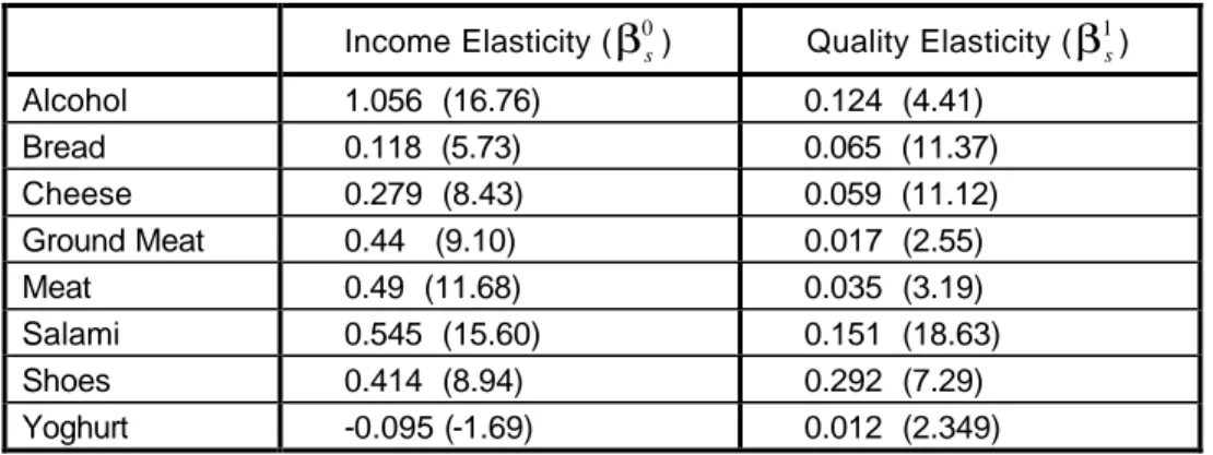
In the first stage we run equations (15) and (16) for each of the eight goods. At this point we are able to estimate the income elasticities (β⁰_s) and the quality elasticities (β¹_s) of the goods (table 2). The t-statistics are given in brackets.

Table 2: Income and quality elasticities

Income Elasticity (β⁰_s) Quality Elasticity (β¹_s)

Alcohol 1.056 (16.76) 0.124 (4.41)

Bread 0.118 (5.73) 0.065 (11.37)

Cheese 0.279 (8.43) 0.059 (11.12)

Ground Meat 0.44 (9.10) 0.017 (2.55)

Meat 0.49 (11.68) 0.035 (3.19)

Salami 0.545 (15.60) 0.151 (18.63)

Shoes 0.414 (8.94) 0.292 (7.29)

Yoghurt -0.095 (-1.69) 0.012 (2.349)

Alcohol clearly comes out as a luxury good. Ground meat, meat, salami, and shoes are reasonably elastic with their income elasticities between 0.45 and 0.55, while bread and cheese are necessities. Yoghurt has a negative income elasticity, but the coefficient is insignificant at the 5% level of significance. Therefore, we conclude that for Bulgaria yoghurt is

(16)

an absolute necessity with an income elasticity equal to zero. The reason behind this finding is that both poor and rich people consume the same amount of yoghurt. For example, pensioners in Bulgaria  the people with the lowest income in the country  inevitably consume at least one container of yoghurt each day, and with an increase in income it is hard to observe an increase in the consumption of yoghurt.

Of considerable interest are the derived quality elasticities. Shoes have the highest quality elasticity  a result that should not be of surprise given the wide range of quality of this good.

Alcohol and salami come next. Bread, cheese, and meat show a small quality elasticity, while ground meat and yoghurt show almost none at all. This is mainly due to the lack of a large variety of available brands. For example, in 1992, cow yoghurt was the predominant brand and one could hardly find any of the other two or three brands.

5.2. Second Stage

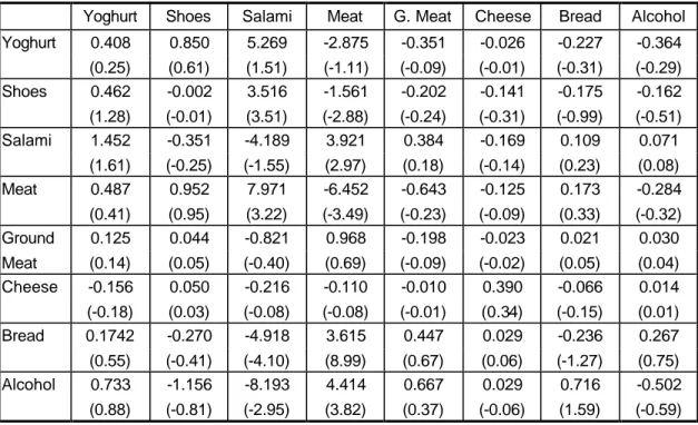
In the second stage, we use the output from the first stage to derive the own- and cross-price elasticities of the goods in the specified demand system. First, we generate the corrected quantities and unit values according to (17) and (18) and use them to generate the matrices S and R as given by equations (21) and (22). Second, we generate the Ω^andΓ matrices, which would be used to correct for the likely measurement error.

A very rough estimate of the price elasticities would be the matrix ~

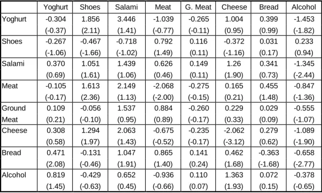
S⁻¹R. However, we need to correct for the measurement error, therefore we calculate Β~ according to (25). Without taking into account the quality effect, Β~ would be the matrix of the price elasticities (table 3). From table 2, though, it is evident that the quality elasticity is significantly different from zero for all goods, and as a result of this the matrix of own- and cross-price elasticities should be estimated according to (28). The output is given in table 4 with the corresponding t-statistics listed in the brackets.

(17)

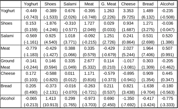
Table 3: The own- and cross-price elasticities without the quality effect taken into account, 1992

Yoghurt Shoes Salami Meat G. Meat Cheese Bread Alcohol Yoghurt -0.449 -0.389 0.676 -0.395 1.263 3.353 1.489 -0.235

(-0.743) (-1.533) (2.026) (-0.748) (2.226) (9.725) (6.132) (-0.508) Shoes 0.153 -1.876 -0.310 1.727 0.029 0.934 1.271 -0.036

(0.159) (-4.246) (-0.577) (2.049) (0.033) (1.687) (3.275) (-0.047) Salami -0.569 0.925 1.018 -0.092 1.251 0.241 0.531 0.520

(-1.161) (4.540) (3.771) (-0.215) (2.726) (0.864) (2.698) (1.386) Meat -0.779 -0.429 0.388 0.335 -0.429 2.027 1.964 0.507

(-1.183) (-1.427) (1.066) (0.579) (-0.679) (5.244) (7.406) (0.991) Ground -0.141 0.146 0.335 2.677 0.114 -1.017 0.303 -0.205 Meat (-0.244) (0.594) (1.049) (5.332) (0.210) (-3.081) (1.309) (-0.462) Cheese 0.172 -0.588 0.011 1.171 -0.579 -0.895 0.909 0.445

(0.103) (-0.820) (0.012) (0.816) (-0.373) (-0.941) (1.354) (0.347) Bread 0.205 -0.373 -0.016 -0.263 0.211 0.821 -1.638 -0.180

(0.490) (-2.131) (-0.070) (-0.721) (0.537) (3.438) (-9.704) (-0.563) Alcohol -0.065 1.413 0.299 -0.973 0.690 -1.350 -0.417 -0.775

(-0.213) (10.913) (1.765) (-3.703) (2.450) (-7.692) (-3.424) (-3.333)

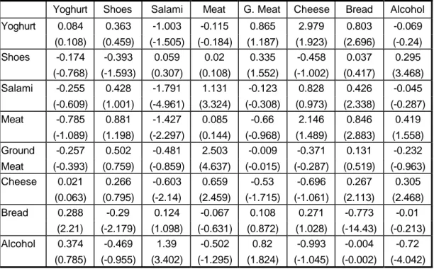
Table 4: The matrix of own- and cross-price elasticities, 1992

Yoghurt Shoes Salami Meat G. Meat Cheese Bread Alcohol Yoghurt 0.084 0.363 -1.003 -0.115 0.865 2.979 0.803 -0.069

(0.108) (0.459) (-1.505) (-0.184) (1.187) (1.923) (2.696) (-0.24) Shoes -0.174 -0.393 0.059 0.02 0.335 -0.458 0.037 0.295 (-0.768) (-1.593) (0.307) (0.108) (1.552) (-1.002) (0.417) (3.468) Salami -0.255 0.428 -1.791 1.131 -0.123 0.828 0.426 -0.045 (-0.609) (1.001) (-4.961) (3.324) (-0.308) (0.973) (2.338) (-0.287) Meat -0.785 0.881 -1.427 0.085 -0.66 2.146 0.846 0.419

(-1.089) (1.198) (-2.297) (0.144) (-0.968) (1.489) (2.883) (1.558) Ground -0.257 0.502 -0.481 2.503 -0.009 -0.371 0.131 -0.232 Meat (-0.393) (0.759) (-0.859) (4.637) (-0.015) (-0.287) (0.519) (-0.963) Cheese 0.021 0.266 -0.603 0.659 -0.53 -0.696 0.267 0.305

(0.063) (0.795) (-2.14) (2.459) (-1.715) (-1.061) (2.113) (2.468) Bread 0.288 -0.29 0.124 -0.067 0.108 0.271 -0.773 -0.01

(2.21) (-2.179) (1.098) (-0.631) (0.872) (1.028) (-14.43) (-0.213) Alcohol 0.374 -0.469 1.39 -0.502 0.82 -0.993 -0.004 -0.72

(0.785) (-0.955) (3.402) (-1.295) (1.824) (-1.045) (-0.002) (-4.042)

(18)

Let us first discuss the results in table 4. Twenty-five out of the sixty-four coefficients are significant. Two of the own-price elasticities are positive  those of yoghurt and meat  but they are not significantly different from zero. The other own-price elasticities have the expected negative sign, although the coefficients for ground meat and cheese are insignificant. Salami seems to be highly elastic. Bread and alcohol are also price elastic, while shoes are less so.

Cheese, yoghurt, ground meat and meat seem to be price inelastic. The finding that yoghurt and cheese are price inelastic can be attributed to the fact that they are a fundamental part of the menu of the individual household, and despite any price changes the households keep consuming the same quantities of these goods. It is difficult, however, to provide a rationale for the observed negligible own-price elasticity of meat and ground meat.

Let us now turn to the cross-price elasticities listed in table 4. There are a few interesting results which need to be emphasised. First, there is a strong substitutability of yoghurt for cheese: an increase in the price of cheese increases substantially the quantity of yoghurt consumed. The opposite, however, is not true: the price of yoghurt has no influence whatsoever on the consumption of cheese. This result is reasonable given that cheese is more expensive than yoghurt. A higher cheese price thus enables the consumer to substitute with yoghurt, while a higher price for yoghurt does not enable him to switch to cheese.

Second, the pattern of the cross-price elasticities of salami, meat and ground meat is quite interesting. Meat is the most expensive of these goods. A higher price for meat therefore increases the consumption of salami and ground meat since people switch to these goods. An increase in the price of salami, however, decreases the consumption of meat and ground meat since people cannot switch to these more expensive products and stop consuming them altogether.

Third, yoghurt, salami, meat, and cheese are substitutes for bread  that is, an increase in the price of bread increases the consumption of these goods. The opposite is not true as bread shows to be a substitute only for yoghurt.

Finally, an increase in the price of alcohol increases the consumption of shoes, meat, and cheese and has no effect on the consumption of other goods. Therefore shoes, meat, and cheese are substitutes to alcohol, while alcohol is a substitute for salami and ground meat.

As indicated above, the difference between the Β~ and the Θ~ matrices comes from the quality effect. If the quality elasticity is close to zero, the elasticity from the Β~ matrix should be almost the same as that in the Θ~ matrix. We found no quality effect for yoghurt, and from tables 3 and 4 we see that both coefficients are not significantly different from zero. The same is true for meat, ground meat, and cheese. Despite the relatively high quality elasticity, alcohol reveals almost the same price elasticity due to its high income elasticity. There is a substantial reduction in the elasticity of bread and shoes due to their high quality elasticity  especially the one for shoes.

(19)

We construct a formal test for the symmetry of the substitution matrices underlying the uncompensated elasticities (tables 4, 6, 7, 9, 10). If the uncompensated own- or cross-price elasticity is θij then the compensated elasticity εij is given by

ε_ij =θ_ij +β_i⁰s_j, (29)

where sj is the budget share of good j in the total expenditure. The substitution matrix will be symmetrical if and only if siεij is symmetrical, which is equivalent to s_iθ_ij +β_i⁰s s_i _j^being

symmetrical. Since the second term of the above expression is small, the sign of θij

determines complements and substitutes. We test the restriction at the sample means for the budget shares. In this case we obtain the following set of restrictions for the Θ matrices and β⁰ vectors for the years 1992 and 1993.

s_iθ_ij +β_i⁰s s_i _j =s_jθ_ij +β⁰_{j i}s s_j^, i,j = 1,8, i≠ j. (30)

Further, we define a 72-element vector α^'=[vec( ) ,Θ ^' β⁰^')] with a variance-covariance matrix V_α, which is a matrix with the following structure:

V V vec Cov vec

Cov vec Var

α

β

β β

=

 



cov[ ( )] [ ( ), ]

{ [ ( ), ]}^' [ ]

Θ Θ

Θ

0

0 0 (31)

The symmetry restrictions take the form

Rα = 0 , (32)

where R is a (28x72) matrix of restrictions. Symmetry can be tested by examining the vector

Rα~ (the tilde stays for the estimated values) and using its variance-covariance matrix RV_αR^’ to construct standard errors and t-tests. We obtain an overall Wald test by calculating

~^' ^'( ^') ~

α R RV R_α ⁻¹Rα, which, under the null hypothesis of symmetry, is asymptotically distributed as a χ² distribution with sixteen degrees of freedom.

The Wald statistic is 92.85 for 1992 and 103.65 for 1993, both of which are highly significant both at 5% and 1% levels. The critical value for the chi-squared distribution with sixteen degrees of freedom is 28.85 at the 5% level and 32 at the 1% level of significance. Hence, we conclude that the hypothesis of symmetry is not accepted.

(20)

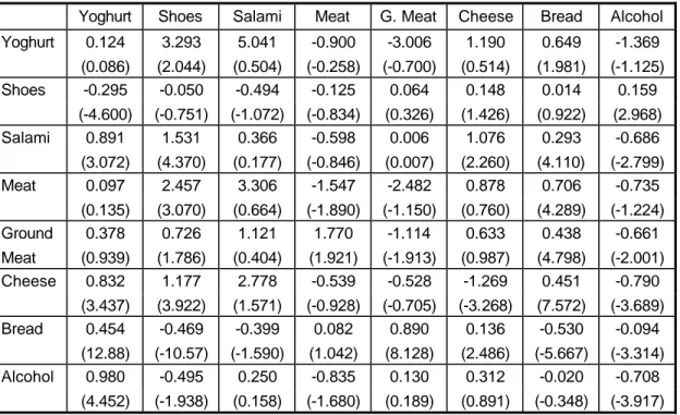
5.3. The Dynamics of Income, Own- and Cross-Price Elasticities in 1992 and 1993

5.3.1. Income and Quality Elasticities

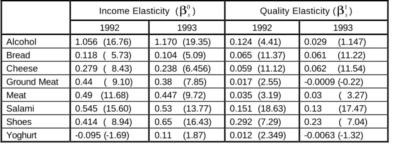
Table 5 lists the income and quality elasticities for 1992 and 1993. The corresponding t- statistics are shown in brackets.

Alcohol remains a luxury good with its income elasticity rising slightly from 1.056 in 1992 to 1.170 in 1993. Ground meat, meat, and salami remain reasonably elastic goods, although their income elasticities fall slightly. Bread and cheese continue to reveal themselves as necessities, with their elasticities in 1993 being slightly lower as well. Shoes show a 60%

increase in income elasticity. Yoghurt remains an absolute necessity  its coefficient is insignificant at the 5% level of significance. The reason behind this finding is that yoghurt is part of the traditional Bulgarian cuisine and people consume the same amount of yoghurt despite any changes in their income levels.

Table 5: Income and quality elasticities for 1992 and 1993

Income Elasticity (β⁰_s) Quality Elasticity (β¹_s)

1992 1993 1992 1993

Alcohol 1.056 (16.76) 1.170 (19.35) 0.124 (4.41) 0.029 (1.147) Bread 0.118 ( 5.73) 0.104 (5.09) 0.065 (11.37) 0.061 (11.22) Cheese 0.279 ( 8.43) 0.238 (6.456) 0.059 (11.12) 0.062 (11.54) Ground Meat 0.44 ( 9.10) 0.38 (7.85) 0.017 (2.55) -0.0009 (-0.22) Meat 0.49 (11.68) 0.447 (9.72) 0.035 (3.19) 0.03 ( 3.27) Salami 0.545 (15.60) 0.53 (13.77) 0.151 (18.63) 0.13 (17.47) Shoes 0.414 ( 8.94) 0.65 (16.43) 0.292 (7.29) 0.23 ( 7.04) Yoghurt -0.095 (-1.69) 0.11 (1.87) 0.012 (2.349) -0.0063 (-1.32)

The dynamics of the quality elasticities presents some interesting findings as well. Shoes continue to have the highest quality elasticity  around 0.23  due to the wide range of quality of this good. Salami, for the same reason, comes next. Bread, cheese, and meat keep their low quality elasticity, while ground meat and yoghurt still show none at all. This is mainly due to the fact that the variety of these goods in 1993 was as limited as in 1992. Quite surprising is the change in the coefficient of alcohol  from a good with a high quality elasticity in 1992 it becomes a good with no quality elasticity at all in 1993. One possible explanation for this phenomenon is the emergence of faked copies of the high-quality brands, which diverted people from buying them. Another possibility is the existence of “brand loyalty” especially among older people.

(21)

5.3.2. Own- and Cross-Price Elasticities

Tables 5 and 6 list the own- and cross-price elasticities for 1992 and 1993, respectively, with the corresponding t-statistics shown in brackets.

Let us first discuss the own-price elasticities. Alcohol reveals a stable own-price elasticity, while the one for bread slightly falls most probably due to the fact that in 1993 bread became a more fundamental (for the Bulgarian consumer) good than in 1992. The own-price elasticities of cheese, ground meat, and meat become significant, while the one for salami becomes insignificant. The elasticity of yoghurt is still insignificant. The finding that yoghurt is price inelastic can be attributed to the fact that it is a fundamental part of the menu of the individual household, and despite any price changes households keep consuming the same quantity.

The elasticity of shoes becomes insignificant in 1993.

Table 6: The matrix of own- and cross-price elasticities in 1992

Yoghurt Shoes Salami Meat G. Meat Cheese Bread Alcohol Yoghurt 0.084 0.363 -1.003 -0.115 0.865 2.979 0.803 -0.069

(0.108) (0.459) (-1.505) (-0.184) (1.187) (1.923) (2.696) (-0.24) Shoes -0.174 -0.393 0.059 0.02 0.335 -0.458 0.037 0.295 (-0.768) (-1.593) (0.307) (0.108) (1.552) (-1.002) (0.417) (3.468) Salami -0.255 0.428 -1.791 1.131 -0.123 0.828 0.426 -0.045

(-0.609) (1.001) (-4.961) (3.324) (-0.308) (0.973) (2.338) (-0.287) Meat -0.785 0.881 -1.427 0.085 -0.66 2.146 0.846 0.419

(-1.089) (1.198) (-2.297) (0.144) (-0.968) (1.489) (2.883) (1.558) Ground -0.257 0.502 -0.481 2.503 -0.009 -0.371 0.131 -0.232 Meat (-0.393) (0.759) (-0.859) (4.637) (-0.015) (-0.287) (0.519) (-0.963) Cheese 0.021 0.266 -0.603 0.659 -0.53 -0.696 0.267 0.305

(0.063) (0.795) (-2.14) (2.459) (-1.715) (-1.061) (2.113) (2.468) Bread 0.288 -0.29 0.124 -0.067 0.108 0.271 -0.773 -0.01

(2.21) (-2.179) (1.098) (-0.631) (0.872) (1.028) (-14.43) (-0.213) Alcohol 0.374 -0.469 1.39 -0.502 0.82 -0.993 -0.004 -0.72

(0.785) (-0.955) (3.402) (-1.295) (1.824) (-1.045) (-0.002) (-4.042)

The pattern of the cross-price elasticities is different in the two years. Yoghurt has many more substitutes in 1993 than in 1992. Bread remains a substitute to yoghurt, but now alcohol, salami, and, as expected, cheese obtain significant cross-price elasticities. The price of shoes seems to affect all other goods in the demand system. This finding shows that the prices of luxury goods in 1993 were no longer irrelevant to the consumer. The pattern of the cross-price elasticities between salami, meat, and ground meat changes. In 1992 meat was the most expensive of these goods; therefore, a higher price for meat increased the consumption of salami and ground meat since people switched to these goods. An increase in the price of