ATLAS-CONF-2017-003 08February2017
ATLAS CONF Note
ATLAS-CONF-2017-003
Measurement of longitudinal flow correlations in Pb+Pb collisions at √
sNN =2.76 and 5.02 TeV with the ATLAS detector
The ATLAS Collaboration
2nd February 2017
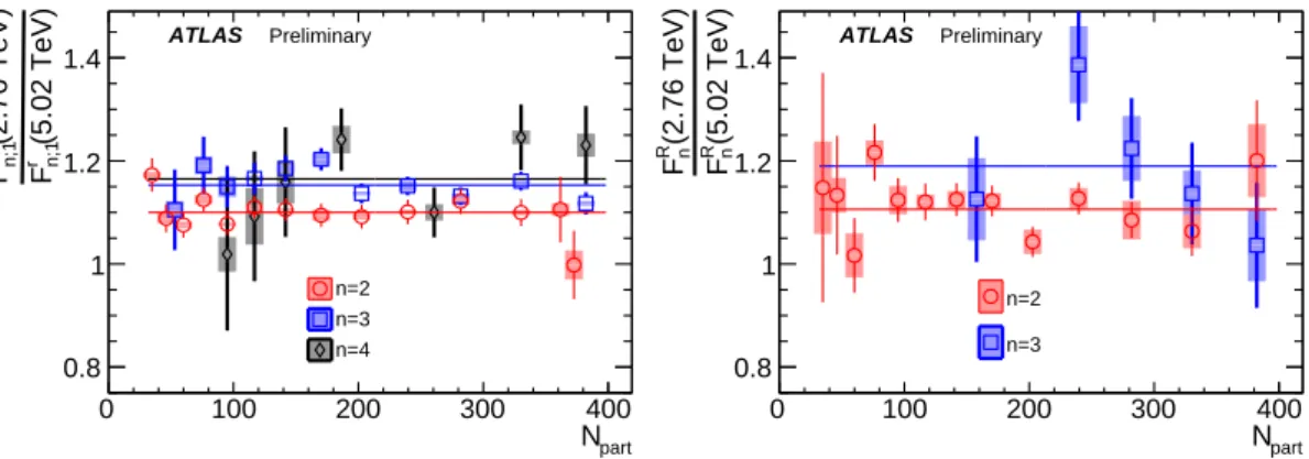
Measurements of longitudinal flow correlations are presented for charged particles in the pseudorapidity range∣η∣ <2.4 using 7µb−1and 22–470µb−1of Pb+Pb collisions at√sNN= 2.76 and 5.02 TeV, respectively, with the ATLAS detector at the LHC. It is found that the correlation between the harmonic flow coefficientsvnmeasured in two separatedηintervals does not factorize into the product of single-particlevn, and this breaking of factorization, or flow decorrelation, increases linearly with theη separation between the intervals. The linear coefficients of the flow decorrelation are found to be larger at 2.76 TeV than 5.02 TeV. Higher-order moments of the correlations are also measured, and the corresponding linear coefficients for thekth-moment of thevnare found to scale withk forn>2, but scale faster than k for n = 2. The decorrelation effect is separated into contributions from the magnitude of vn changing withη and the event-plane orientation changing with η. These two contributions are found to be comparable. The longitudinal flow correlations are also measured betweenvn of different order inn. The longitudinal fluctuations ofv2 andv3 are found to be independent of each other, while the longitudinal fluctuations ofv4 andv5 are found to be driven by the non-linear contribution fromv22andv2v3, respectively.
©2017 CERN for the benefit of the ATLAS Collaboration.
Reproduction of this article or parts of it is allowed as specified in the CC-BY-4.0 license.
1 Introduction
Heavy-ion collisions at RHIC and the LHC create hot, dense matter whose space-time evolution is well described by relativistic viscous hydrodynamics [1,2]. Owing to strong event-by-event (EbyE) density fluctuations in the initial state, the space-time evolution of the produced matter also fluctuates event by event. These fluctuations lead to correlations of particle multiplicity in momentum space in both the transverse and longitudinal directions with respect to the collision axis. Studies of the particle correlation in the transverse plane have revealed strong harmonic modulation of the particle densities in the azimuthal angle: dN/dφ ∝1+2∑∞n=1vncosn(φ−Φn), wherevnandΦnrepresent the magnitude and event-plane angle of thenth-order harmonic flow. The measurements of harmonic flow coefficientsvnand their EbyE fluctuations [3–5], as well as the correlations betweenΦnof different order [6–9], have placed important constraints on the properties of the medium, and of transverse density fluctuations in the initial state.
The majority of previous flow studies assumed that the initial condition and space-time evolution of the matter are boost invariant in the longitudinal direction. Recent model studies of two-particle correlations as a function of pseudorapidity η revealed strong EbyE fluctuations of the flow magnitude and phase between two well separated pseudorapidities, i.e. vn(η1) ≠ vn(η2)(forward-backward asymmetry) and Φn(η1) ≠ Φn(η2)(event-plane twist) [10,11]. The CMS Collaboration proposed an observable based on the ratio of correlations betweenηor−ηwith a common reference pseudorapidityηref in the forward direction, and this observable is sensitive to longitudinal correlations betweenηand−η[12]. The CMS results show that the longitudinal fluctuations lead to a linear decrease of the ratio withη, and the slope of the decrease shows a strong centrality dependence for elliptic flow v2 but very weak dependences forv3 and v4. Motivated by this measurement, several new observables have been proposed based on multi-particle correlations in two or moreηintervals [13]. These observables are sensitive to the EbyE fluctuations, as a function ofη, of the initial condition as well as the non-linear mode-mixing effects.
Measurement of these observables can provide new insights on the initial condition along the longitudinal direction, and will help in the development of full three-dimensional viscous hydrodynamic models.
Using these new observables, this note develops further the study of the longitudinal dynamics of col- lective flow in three ways. Firstly, the CMS measurement, which is effectively the first moment of the correlation between flow in separateηintervals, is extended to second and third moments. Secondly, a correlation between four subevents in differentηintervals is measured to separate the contribution from fluctuation ofvnamplitude and contribution from fluctuation ofΦn. Thirdly, measurements are also made of the correlations between harmonics of different order, e.g. between v2 and v4 in different η inter- vals, to investigate how the mode-mixing effects evolve with rapidity. In this way, this note presents a comprehensive measurement of flow decorrelation involvingv2,v3,v4andv5, using Pb+Pb collisions at
√sNN=2.76 and 5.02 TeV.
2 Observables
This section gives a brief summary of the observables measured in this note, and the mathematical details can be found in Ref. [13,14]. The azimuthal anisotropy of the particle production in an event is described by harmonic flow vectorsun = vneinΦn, wherevn andΦn are the magnitude and phase (or event plane), respectively. They are estimated from the observed per-particle normalized flow vectorqn:
qn≡ ∑iwieinφi
∑ wi ≡qneinΨn (1)
The sum runs over all particles in a givenηinterval of the event andwi is the weight assigned to theith particle. The weight accounts for detector non-uniformity and tracking inefficiency.
The longitudinal flow fluctuations are studied using the correlation between thekth-moment of the nth- order flow vectors in two differentηintervals, averaged over events in a given centrality interval,rn∣n;k:
rn∣n;k(η) = ⟨qkn(−η)q∗nk(ηref)⟩
⟨qkn(η)q∗nk(ηref)⟩ =⟨[vn(−η)vn(ηref)]kcoskn(Φn(−η) −Φn(ηref))⟩
⟨[vn(η)vn(ηref)]kcoskn(Φn(η) −Φn(ηref))⟩ (2) where the subscript “n∣n;k” denotes thekthmoment of the flow vector of ordernat±ηand thekthmoment of the complex conjugate of the flow vector of ordernatηref, and theηref is the reference pseudorapidity common to the numerator and the denominator. This correlator is sensitive to the flow decorrelation betweenηand−η through the reference flow vector qkn(ηref). The detector effects associated with the referenceηrange are expected to be largely cancelled out in the ratio.
To ensure a sizable pseudorapidity gap between the two flow vectors in the numerator and denominator of Eq.2,ηrefis usually chosen to be at large pseudorapidity, e.g.ηref >4, while the pseudorapidity ofqn(−η) andqn(η)is usually chosen to be close to mid-rapidity,∣η∣ <2.5. If flow harmonics from multi-particle correlations factorize into single-particle flow harmonics, e.g.⟨ukn(η)u∗nk(ηref)⟩ = ⟨vkn(η)⟩ ⟨vkn(ηref)⟩, then it is expected thatrn∣n;k(η) =1. Therefore a value ofrn∣n;k(η)different from one implies a factorization- breaking effect due to longitudinal flow fluctuations, and such an effect is generally referred to as “flow decorrelation”.
Based on the CMS measurement [12] and arguments in Ref. [13], the observable rn∣n;k(η) is expected to be approximately a linear function of ηwith a negative slope, and is sensitive to both the forward- backward (FB) asymmetry in the magnitude ofvn, e.g.vn(−η) ≠vn(η), and to the twist of the event-plane angles betweenηand−η:
rn∣n;k(η) ≈1−2kFn;kr η, Fn;kr =Fasyn;k +Ftwin;k (3) whereFn;kasyandFn;ktwirepresent the contribution from FBvnasymmetry and event-plane twist, respectively.
Results onrn∣n;k have been obtained by the CMS collaboration fork=1 andn=2–4. The measuredFn;1r show only a weak dependence onηref forηref >3 at the LHC. Measuring rn∣n;k fork >1 can yield new information on how thevnasymmetry and event-plane twist fluctuate event by event.
IfFn;kasyandFn;ktwiin Eq.3are also independent ofk, i.e. Fn;kasy=FnasyandFn;ktwi=Ftwin , then:
rn∣n;k≈rkn∣n;1 . (4)
Deviation from this relation is sensitive to detailed EbyE structure of the flow fluctuations in the longit- udinal direction.
To separate the contributions of the asymmetry and twist effects, a new observable involving correlations of flow vectors in fourηintervals is required,
Rn,n∣n,n(η) = ⟨qn(−ηref)qn(−η)q∗n(η)q∗n(ηref)⟩
⟨qn(−ηref)q∗n(−η)qn(η)q∗n(ηref)⟩
= ⟨vn(−ηref)vn(−η)vn(η)vn(ηref)cosn[Φn(−ηref) −Φn(ηref) + (Φn(−η) −Φn(η))]⟩
⟨vn(−ηref)vn(−η)vn(η)vn(ηref)cosn[Φn(−ηref) −Φn(ηref) − (Φn(−η) −Φn(η))]⟩
(5)
The effect of asymmetry is the same in both numerator and denominator, and so this correlator is mainly sensitive to the event-plane twist effects:
Rn,n∣n,n≈1−4Ftwin;2η . (6) Therefore the two contributions can be separated by combiningrn∣n;2andRn,n∣n,nvia Eqs.3and6.
Measurements of longitudinal flow fluctuations can also be extended to correlations between harmonics of different order:
r2,3∣2,3(η) = ⟨q2(−η)q∗2(ηref)q3(−η)q∗3(ηref)⟩
⟨q2(η)q∗2(ηref)q3(η)q∗3(ηref)⟩ (7) r2,2∣4(η) = ⟨q22(−η)q∗4(ηref)⟩ + ⟨q22(ηref)q∗4(−η)⟩
⟨q22(η)q∗4(ηref)⟩ + ⟨q22(ηref)q∗4(η)⟩ (8) r2,3∣5(η) = ⟨q2(−η)q3(−η)q∗5(ηref)⟩ + ⟨q2(ηref)q3(ηref)q∗5(−η)⟩
⟨q2(η)q3(η)q∗5(ηref)⟩ + ⟨q2(ηref)q3(ηref)q∗5(η)⟩ (9) If the longitudinal fluctuations forv2andv3are independent of each other, one would expectr2,3∣2,3=r2∣2;1r3∣3;1. On the other hand,r2,2∣4 andr2,3∣5 are sensitive to theηdependence of the correlations between vn and event planes of different order, for example⟨q22(−η)q∗4(ηref)⟩ = ⟨v22(−η)v4(ηref)cos 4(Φ2(−η) −Φ4(ηref))⟩. Correlations between different orders have been measured previously at the LHC [4,5,15].
It is well established that theu4andu5in Pb+Pb collisions contain a linear contribution associated with initial geometry and mode-mixing contributions from lower-order harmonics due to non-linear hydro- dynamic response [4,5,16–18]:
u4=u4L+β2,2u22, u5=u5L+β2,3u2u3, (10) where the linear componentunLis driven by the corresponding eccentricitynin the initial geometry [19].
If the linear component of v4 and v5 is uncorrelated with lower-order harmonics, i.e. u22u∗4L ∼ 0 and u2u3u∗5L∼0, one expects:
r2,2∣4≈r2∣2;2, r2,3∣5≈r2,3∣2,3. (11) Furthermore, thern∣n;1correlators involvingv4andv5can be approximated by:
r4∣4;1(η) ≈ ⟨u4L(−η)u∗4L(ηref)⟩ +β22,2⟨u22(−η)u∗22(ηref)⟩
⟨u4L(η)u∗4L(ηref)⟩ +β22,2⟨u22(η)u∗22(ηref)⟩ (12) r5∣5;1(η) ≈ ⟨u5L(−η)u∗5L(ηref)⟩ +β22,3⟨u2(−η)u∗2(ηref)u3(−η)u∗3(ηref)⟩
⟨u5L(η)u∗5L(ηref)⟩ +β22,3⟨u2(η)u∗2(ηref)u3(η)u∗3(ηref)⟩ (13) Therefore, both the linear and non-linear components may be important forr4∣4;1andr5∣5;1.
3 ATLAS detector and trigger
The ATLAS detector [20] provides nearly full solid-angle coverage of the collision point with tracking detectors, calorimeters, and muon chambers, and is well suited for measurement of multi-particle correl-
ations over a large pseudorapidity range.1 The measurements were performed using the inner detector (ID), minimum-bias trigger scintillators (MBTS), the forward calorimeter (FCal), and the zero-degree calorimeters (ZDC). The ID detects charged particles within∣η∣ < 2.5 using a combination of silicon pixel detectors, silicon microstrip detectors (SCT), and a straw-tube transition radiation tracker (TRT), all immersed in a 2 T axial magnetic field [21]. An additional pixel layer, the “Insertable B Layer”
(IBL) [22,23] installed between Run 1 and Run 2 (2013–2015), is used in the 5.02 TeV Pb+Pb measure- ments. The MBTS system detects charged particles over 2.1≲ ∣η∣ ≲3.9 using two hodoscopes of counters positioned atz= ±3.6 m. The FCal consists of three sampling layers, longitudinal in shower depth, and covers 3.2< ∣η∣ <4.9. The ZDC, available in the Pb+Pb and p+Pb runs, are positioned at±140 m from the collision point, detecting neutrons and photons with∣η∣ >8.3.
This analysis uses approximately 7 µb−1 and 22–470 µb−1 of Pb+Pb data at √sNN = 2.76 TeV and
√sNN =5.02 TeV, respectively, recorded by the ATLAS experiment at the LHC. The 2.76 TeV Pb+Pb data were collected in 2010, while the 5.02 TeV Pb+Pb data were collected in 2015.
The ATLAS trigger system [24] consists of a Level-1 (L1) trigger implemented using a combination of dedicated electronics and programmable logic, and a high-level trigger (HLT) implemented in processors.
The trigger requires signals in two ZDCs or either of the two MBTS counters. The ZDC trigger thresholds on each side are set below the peak corresponding to a single neutron. A timing requirement based on signals from each side of the MBTS is imposed to remove beam backgrounds. This trigger selects 7µb−1 and 22µb−1 of minimum bias Pb+Pb data at √sNN = 2.76 TeV and √sNN = 5.02 TeV, respectively.
To increase the statistics for very central Pb+Pb collisions, a dedicated L1 trigger is used in 2015 to select events with total transverse energy (ΣET) in FCal above 4.54 TeV. This ultra-central trigger samples 470µb−1of Pb+Pb collisions at 5.02 TeV, corresponding to 0–0.1% ultra-central collisions (see Sec.4).
4 Event and track selection
The offline event selection for the Pb+Pb data requires a reconstructed vertex with itszposition satisfying
∣zvtx∣ <100 mm. The selection also requires a time difference∣∆t∣ <3 ns between signals in the MBTS trigger counters on either side of the nominal centre of ATLAS to suppress non-collision backgrounds.
A coincidence between the ZDC signals at forward and backward pseudorapidity is required to reject a variety of background processes, while maintaining high efficiency for inelastic processes. The fraction of events containing more than one inelastic interaction (pile-up) is negligible in 2.76 TeV Pb+Pb collisions, and is estimated to be less than 0.1% for 5.02 TeV Pb+Pb collisions. The pile-up contribution is studied by exploiting the correlation between the transverse energy measured in the FCalΣET or the number of neutrons Nn in the ZDC and the number of tracks associated with a primary vertexNchrec. Since the distribution ofΣET orNnin events with pileup is broader than that for the events without pileup, pile-up events are suppressed by a simple cut on the high tail-end of theΣETorNndistribution as a function of Nchrec.
The Pb+Pb event centrality [25] is characterized using the ΣET deposited in the FCal over the pseu- dorapidity range 3.2< ∣η∣ <4.9 at the electromagnetic energy scale [26]. The FCalΣET distribution is divided into a set of variable percentile bins. A centrality interval refers to a percentile range, starting at
1ATLAS uses a right-handed coordinate system with its origin at the nominal interaction point (IP) in the centre of the detector and thez-axis along the beam pipe. The x-axis points from the IP to the centre of the LHC ring, and they-axis points upward. Cylindrical coordinates(r, φ)are used in the transverse plane,φbeing the azimuthal angle around the beam pipe.
The pseudorapidity is defined in terms of the polar angleθasη= −ln tan(θ/2).
0% relative to the most central collisions. Thus the 0–5% centrality interval, for example, corresponds to the most central 5% of the events. The ultra-central trigger mentioned in Sec.3selects events in 0–0.1%
centrality with full efficiency. A Monte Carlo Glauber analysis [25,27] is used to estimate the average number of participating nucleons,Npart, for each centrality interval. The systematic uncertainty onNpart is less than 1% for centrality intervals in the range of 0–20% and increases to 6% for centrality intervals in the range of 70–80%. The Glauber model also provides a correspondence between theΣETdistribu- tion and sampling fraction of the total inelastic Pb+Pb cross section, allowing for the setting of centrality percentiles. For this analysis, a selection of collisions corresponding to 0–70% centrality is used to avoid possible biases from diffraction or other processes that contribute to very peripheral collisions. Following the convention of heavy ion analysis, the centrality dependence of the results in this paper is presented as a function ofNpart.
Charged-particle tracks and primary vertices are reconstructed in the ID using algorithms whose im- plementation was improved for Run 2 of the LHC. A special reconstruction procedure, optimized for tracking in dense environments, is used for this purpose [28]. Tracks are required to have pT >0.5 GeV and∣η∣ <2.5. For the 2.76 TeV data, tracks are required to have at least nine hits in the silicon detectors with no missing Pixel hits and not more than one missing SCT hit, taking into account the effects of known dead modules. For the 5.02 TeV data, tracks are required to have at least two pixel hits, with the additional requirement of a hit in the first pixel layer when one is expected, at least eight SCT hits, and at most one missing hit in the SCT. In addition, for both datasets, the point of closest approach of the track is required to be within 1 mm of the primary vertex in both the transverse and longitudinal directions [29].
The efficiency, (pT, η), of the track reconstruction and track selection cuts is evaluated using Pb+Pb Monte Carlo events produced with the HIJING event generator [30]. The generated particles in each event are rotated in azimuthal angle according to the procedure described in Ref. [31] to produce harmonic flow consistent with previous ATLAS measurements [8,32]. The response of the detector is simulated using GEANT4 [33,34] and the resulting events are reconstructed with the same algorithms applied to the data.
For the 5.02 TeV Pb+Pb data, the absolute efficiency increases with pT by 5% between 0.5 GeV and 0.8 GeV, and varies only weakly for pT>0.8 GeV. The efficiency varies more strongly withηand event multiplicity. For pT >0.8 GeV, it ranges from 75% atη≈0 to 50% for∣η∣ >2 in peripheral collisions, while it ranges from 71% atη≈0 to about 40% for∣η∣ >2 in central collisions. The detailed description of tracking efficiency in 5.02 TeV data can be found in Refs. [35]. The tracking efficiency for the 2.76 TeV data has similar dependence onpTandηand is taken from Ref. [36]. However the correlation analysis in this note is not particularly sensitive to the efficiency.
The rate of falsely reconstructed tracks (“fakes”) is also estimated and found to be significant only in central collisions and lowpT, where it ranges from 2% at∣η∣ <1 to 8% at largestη. The fake rate drops rapidly for higherpT and towards more peripheral collisions. The fake rate has been accounted for in the tracking efficency correction following the procedure in Ref. [35].
5 Data analysis
Measurement of the longitudinal flow dynamics requires the calculation of the flow vectorqnvia Eq.1in the ID and the FCal. The flow vector from the FCal serves as the referenceqn(ηref), while the ID provides the flow vector as a function of pseudorapidityqn(η).
In order to account for detector inefficiencies and non-uniformity, particle weight for theith-particle in the ID for the flow vector (Eq.1) is defined as [36]
wIDi (η, φ,pT) =dID(η, φ)/(η,pT). (14) The determination of track efficiency (η,pT) is described in Section4. The additional weight factor dID(η, φ) corrects for variation of tracking efficiency or non-uniformity of detector acceptance as a function of η. For a given η interval of 0.1, the distribution in azimuthal bins, N(φ, η), is built up from all reconstructed charged particles with 0.5 < pT < 3 GeV. The weight factor is then obtained as dID(η, φ) ≡ ⟨N(η)⟩ /N(φ, η), where⟨N(η)⟩is the average of theN(φ, η). This “flattening” procedure re- moves mostφ-dependent non-uniformity from track reconstruction, which is important for any azimuthal correlation analysis. Similarly, the weight in the FCal for the flow vector (Eq.1) is defined as:
wFCali (η, φ) = (ET)idFCal(η, φ) (15) where(ET)i is the transverse energy measured at the ith tower in the FCal at ηand φ. The azimuthal weightdFCal(η, φ)is calculated for eachηinterval of approximately 0.1, in a similar way to what is done for the ID. It ensures that the ET-weighted distribution, averaged over all events in a given centrality interval, is uniform inφ. The flow vectorsqn(η)andqn(ηref)are further corrected by an event-averaged offset,qn≡qn− ⟨qn⟩evts[4].
The flow vectors obtained after these reweighing and offset procedures are used in the correlation analysis.
The correlation quantities used inrn∣n;k are calculated as:
⟨qkn(η)q∗nk(ηref)⟩ ≡ ⟨qkn(η)q∗nk(ηref)⟩s− ⟨qkn(η)q∗nk(ηref)⟩b, (16) where subscripts “s” and “b” represent the correlator constructed from the same event (“signal”) and from the mixed-event (“background”), respectively. The mixed-event quantity is constructed by combin- ing qkn(η) from each event with q∗nk(ηref) obtained in other events with similar centrality (within 1%) and similarzvtx (∣∆zvtx∣ < 5 mm). The⟨qkn(η)q∗nk(ηref)⟩b, which is typically more than two orders of magnitude smaller than the corresponding signal term, is subtracted to account for any residual detector non-uniformity effects that correlate between differentηranges. This mixed-event procedure is used in previous correlation analyses, for example Refs. [4,5].
For correlators involving flow vectors in two differentηranges, mixed events are constructed from two different events. For example, the correlation forr2,3∣5is calculated as:
⟨q2(η)q3(η)q∗5(ηref)⟩ ≡ ⟨q2(η)q3(η)q∗5(ηref)⟩s− ⟨q2(η)q3(η)q∗5(ηref)⟩b. (17) The mixed-event correlator is constructed by combining q2(η)q3(η)from one event with q∗5(ηref) ob- tained in another event with similar centrality (within 1%) and similarzvtx(∣∆zvtx∣ <5 mm). On the other hand, for correlators involving more than two differentηranges, mixed events are constructed from more than two different events, one for each uniqueηrange. One such example isRn,n∣n,n, for which each mixed event is constructed from four different events with similar centrality andzvtx.
Due to the symmetry of the Pb+Pb collision system, most correlators can be symmetrized to improve statistical precision. For example, instead of Eq.2, the actual measured observable is:
rn∣n;k(η) = ⟨qkn(−η)q∗nk(ηref) +qkn(η)q∗nk(−ηref)⟩
⟨qkn(η)q∗nk(ηref) +qkn(−η)q∗nk(−ηref)⟩ (18)
The symmetrization procedure also allows further cancellation of possible differences betweenηand−η in the tracking efficiency or detector acceptance.
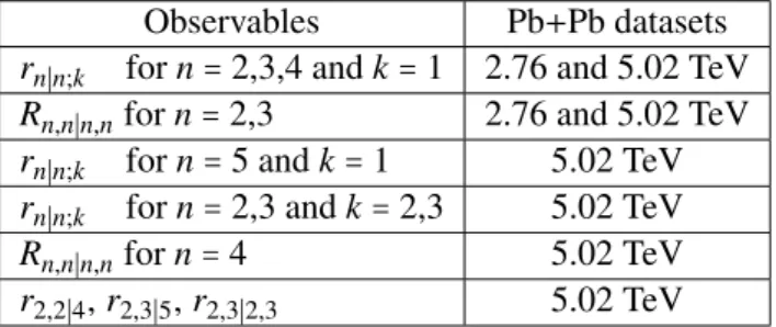
Table1 gives a summary of the set of correlators measured in this note. The analysis is performed in intervals of centrality and the results are presented as a function of η for ∣η∣ < 2.4. The main results are obtained using 5.02 TeV Pb+Pb data. The 2.76 TeV Pb+Pb data are limited, and therefore are used only to obtainrn∣n;1 andRn,n∣n,n to compare with results obtained with the 5.02 TeV data and study the dependence on collision energy.
Table 1: The list of observables measured in this analysis.
Observables Pb+Pb datasets rn∣n;k forn=2,3,4 andk=1 2.76 and 5.02 TeV Rn,n∣n,nforn=2,3 2.76 and 5.02 TeV rn∣n;k forn=5 andk=1 5.02 TeV rn∣n;k forn=2,3 andk=2,3 5.02 TeV Rn,n∣n,nforn=4 5.02 TeV r2,2∣4,r2,3∣5,r2,3∣2,3 5.02 TeV
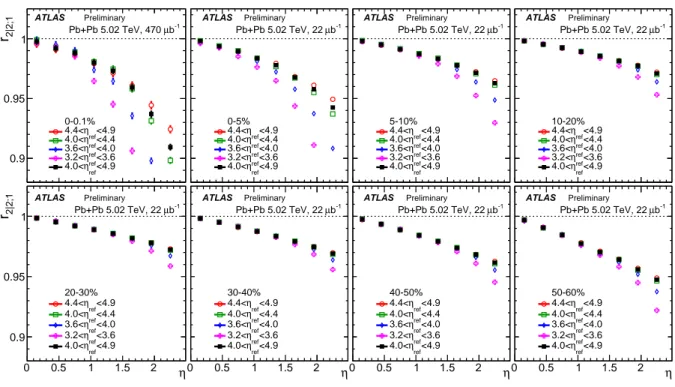
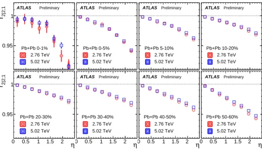
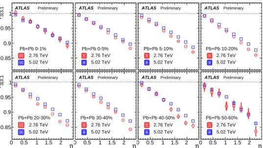
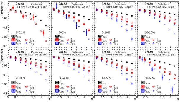
Figures 1 and 2 show the sensitivity of r2∣2;1 and r3∣3;1, respectively, to the choice of reference pseu- dorapidityηref in the FCal. A smallerηref value implies a smaller pseudorapidity gap betweenηandηref. The values of rn∣n;1 generally decrease with decreasingηref, possibly reflecting the contributions from non-flow associated with the away-side jet. However such contributions should be reduced in the most central collisions, due to large charged-particle multiplicity and jet-quenching effects. Therefore the de- crease ofrn∣n;1in the most central collisions could also be due to theηref dependence ofFrn;1, as defined in Eq.3. In this analysis, the reference flow vector is calculated from 4.0< ∣ηref∣ <4.9, which should reduce adequately the effect of dijets and allow good statistical precision. For this choice ofηref range, ther2∣2;1 andr3∣3;1 show a linear decrease as a function of ηin most centrality intervals, indicating a significant breakdown of the factorization of two-particle flow harmonics into single-particle flow harmonics.
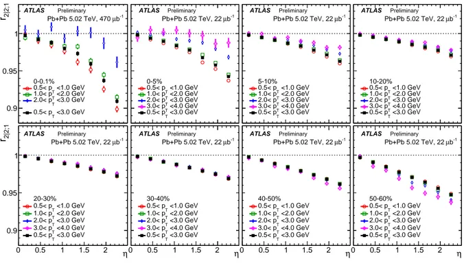
Figures3and4showr2∣2;1andr3∣3;1 calculated for severalpT ranges of the charged particles in the ID.
If the longitudinal flow asymmetry and twist reflect global properties of the event, the values ofrn∣n;1 should not depend strongly on pT. Indeed little dependence is observed, except forr2∣2;1 in the most central collisions and very peripheral collisions. The behaviour in central collisions may be related to the factorization breaking of thev2as a function ofpT [8,12]. The behaviour in peripheral collisions is due to increasing relative contributions from jets and dijets at higherpT and for peripheral collisions. Unless specified otherwise, the measurements presented are performed using charged particles with 0.5<pT<3 GeV.
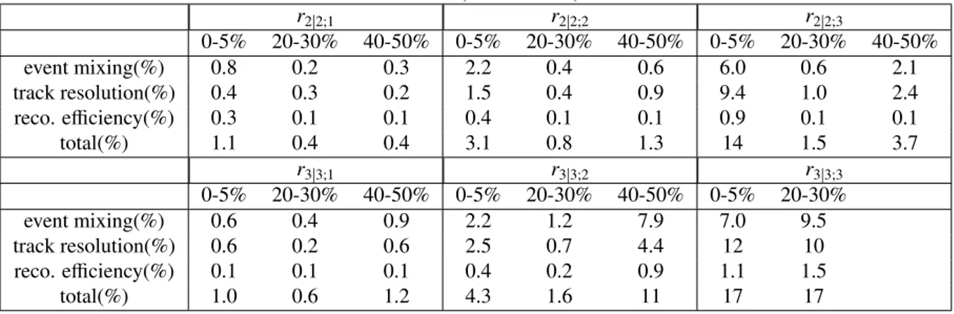
6 Systematic uncertainties
Since all observables are found to follow an approximately linear decrease withη, i.e. D(η) ≈ 1−cη for a given observableD(η)wherecis a constant, the systematic uncertainty is presented as the relative uncertainty for 1−D(η)at η = 1.2, the mid-point of the ηrange. The systematic uncertainties in this analysis arise from the event-mixing, track selection, and reconstruction efficiency. Most of the systematic uncertainties enter the analysis through the particle weights in Eqs.14and15. In general, the uncertainties