h/2 p ELEMENTARYQUANTUMMECHANICS

arXiv:physics/0004072v2 [physics.ed-ph] 29 Apr 2000

Los Alamos Electronic ArXives http://xxx.lanl.gov/physics/0004072

ELEMENTARY QUANTUM MECHANICS

HARET C. ROSU e-mail: rosu@ifug3.ugto.mx

fax: 0052-47187611 phone: 0052-47183089

h/2 π

Copyright c2000 by the author. All commercial rights are reserved.

April 2000

Abstract

This is the first graduate course on elementary quantum mechanics in Inter- net written for the benefit of undergraduate and graduate students. It is a translation (with corrections) of the Romanian version of the course, which I did at the suggestion of several students from different countries. The top- ics included refer to the postulates of quantum mechanics, one-dimensional barriers and wells, angular momentum and spin, WKB method, harmonic oscillator, hydrogen atom, quantum scattering, and partial waves.

CONTENTS

0. Forward ... 4

1. Quantum postulates ... 5

2. One-dimensional rectangular barriers and wells ... 23

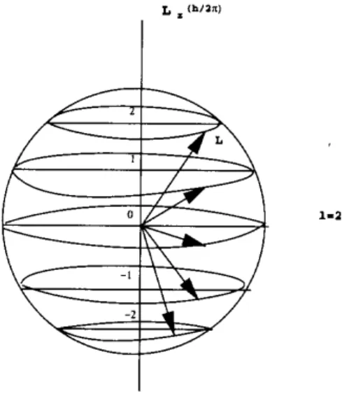
3. Angular momentum and spin ... 45

4. The WKB method ... 75

5. The harmonic oscillator ... 89

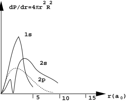
6. The hydrogen atom ... 111

7. Quantum scattering ... 133

8. Partial waves ... 147

There are about 25 illustrative problems.

Spacetime nonrelativistic atomic units a_H = ¯h²/m_ee² = 0.529·10⁻⁸cm t_H = ¯h³/m_ee⁴ = 0.242·10⁻¹⁶sec Planck relativistic units of space and time

lP = ¯h/mPc= 1.616·10⁻³³cm t_P = ¯h/m_Pc² = 5.390·10⁻⁴⁴sec

0. FORWARD

The energy quanta occured in 1900 in the work of Max Planck (Nobel prize, 1918) on the black body electromagnetic radiation. Planck’s “quanta of light” have been used by Einstein (Nobel prize, 1921) to explain the pho- toelectric effect, but the first “quantization” of a quantity having units of action (the angular momentum) belongs to Niels Bohr (Nobel Prize, 1922).

This opened the road to the universalization of quanta, since the action is the basic functional to describe any type of motion. However, only in the 1920’s the formalism of quantum mechanics has been developed in a system- atic manner. The remarkable works of that decade contributed in a decisive way to the rising of quantum mechanics at the level of fundamental theory of the universe, with successful technological applications. Moreover, it is quite probable that many of the cosmological misteries may be disentan- gled by means of various quantization procedures of the gravitational field, advancing our understanding of the origins of the universe. On the other hand, in recent years, there is a strong surge of activity in the information aspect of quantum mechanics. This aspect, which was generally ignored in the past, aims at a very attractive “quantum computer” technology.

At the philosophical level, the famous paradoxes of quantum mechanics, which are perfect examples of the difficulties of ‘quantum’ thinking, are actively pursued ever since they have been first posed. Perhaps the most famous of them is the EPR paradox (Einstein, Podolsky, Rosen, 1935) on the existence ofelements of physical reality, or in EPR words: “If, without in any way disturbing a system, we can predict with certainty (i.e., with probability equal to unity) the value of a physical quantity, then there exists an element of physical reality corresponding to this physical quantity.” Another famous paradox is that of Schr¨odinger’s cat which is related to the fundamental quantum property of entanglement and the way we understand and detect it. What one should emphasize is that all these delicate points are the sourse of many interesting and innovative experiments (such as the so-called

“teleportation” of quantum states) pushing up the technology.

Here, I present eight elementary topics in nonrelativistic quantum me- chanics from a course in Spanish (“castellano”) on quantum mechanics that I taught in the Instituto de F´ısica, Universidad de Guanajuato (IFUG), Le´on, Mexico, during the semesters of 1998.

Haret C. Rosu

1. THE QUANTUM POSTULATES

The following six postulates can be considered as the basis for theory and experiment in quantum mechanics in its most used form, which is known as the Copenhagen interpretation.

P1.- To any physical quantity L, which is well defined at the classical level, one can associate a hermitic operator ˆL.

P2.- To any stationary physical state in which a quantum system can be found one can associate a (normalized) wavefunction. ψ (kψk²_L²= 1).

P3.- In (appropriate) experiments, the physical quantity L can take only the eigenvalues of ˆL. Therefore the eigenvalues should be real, a condition which is fulfilled only by hermitic operators.

P4.- What one measures is always the mean valueLof the physical quantity (i.e., operator) ˆL in a state ψ_n, which, theoretically speaking, is the corresponding diagonal matrix element

hψ_n|Lˆ|ψ_ni=L.

P5.- The matrix elements of the operators corresponding to the cartesian coordinate and momentum,x_bi and_cp_k, when calculated with the wave- functionsf andgsatisfy the Hamilton equations of motion of classical mechanics in the form:

d

dthf |pb_i |gi=−hf | ∂Hb

∂x_bi |gi d

dthf |xb_i|gi=hf | ∂H^b

∂p_bi |gi ,

where H^b is the hamiltonian operator, whereas the derivatives with respect to operators are defined as at point 3 of this chapter.

P6.- The operators p_bi and x_ck have the following commutators:

[p_bi,x_ck] =−i¯hδ_ik, [p_bi,_cp_k] = 0, [x_bi,x_ck] = 0

¯

h=h/2π = 1.0546×10⁻²⁷ erg.sec.

1.- The correspondence between classical and quantum quantities

This can be done by substitutingx_i,p_k withx_{bi c}p_k. The function L is supposed to be analytic (i.e., it can be developed in Taylor series). If the L function does not contain mixed productsx_kp_k, the operator ˆL is directly hermitic.

Exemple:

T = (^P3_i p²_i)/2m −→T^b= (^P3_i p_b²)/2m.

If L contains mixed productsx_ip_i and higher powers of them, ˆLis not hermitic, and in this case L is substituted by ˆΛ, the hermitic part of Lˆ (ˆΛ is an autoadjunct operator).

Exemple:

w(x_i, p_i) =^P_ip_ix_i −→ wb = 1/2^P3_i(p_bix_bi+x_bip_bi).

In addition, one can see that we have no time operator. In quan- tum mechanics, time is only a parameter that can be introduced in many ways. This is so because time does not depend on the canonical variables, merely the latter depend on time.

2.- Probability in the discrete part of the spectrum Ifψn is an eigenfunction of the operator ˆL, then:

L=< n|Lˆ|n >=< n|λn|n >=λn< n|n >=δnnλn=λn. Moreover, one can prove thatL^k= (λn)^k.

If the functionφis not an eigenfunction of ˆL, one can make use of the expansion in the complete system of eigenfunctions of ˆL to get:

Lψˆ _n=λ_nψ_n, φ=^P_na_nψ_n and combining these two relationships one gets:

Lφˆ =^P_nλ_na_nψ_n.

In this way, one is able to calculate the matrix elements of the operator L:ˆ

hφ|Lˆ |φi=^P_n,ma^∗_ma_nλ_nhm|ni=^P_m|a_m|² λ_m,

telling us that the result of the experiment is λ_m with a probability

|am |².

If the spectrum is discrete, according to P4 this means that |a_m |², that is the coefficients of the expansion in a complete set of eigenfunc- tions, determine the probabilitities to observe the eigenvalueλn. If the spectrum is continuous, using the following definition

φ(τ) =^R a(λ)ψ(τ, λ)dλ,

one can calculate the matrix elements in the continuous part of the spectrum

hφ|Lˆ |φi

=^R dτ^Ra^∗(λ)ψ^∗(τ, λ)dλ^R µa(µ)ψ(τ, µ)dµ

=^{R R} a^∗a(µ)µ^R ψ^∗(τ, λ)ψ(tau, µ)dλdµdτ

=^{R R} a^∗(λ)a(µ)µδ(λ−µ)dλdµ

=^R a^∗(λ)a(λ)λdλ

=^R |a(λ)|²λdλ.

In the continuous case,|a(λ)|² should be understood as the probabil- ity density for observing the eigenvalueλbelonging to the continuous spectrum. Moreover, the following holds

L=hφ|Lˆ|φi.

One usually says that hµ | Φi is the representation of | Φi in the representation µ, where |µi is an eigenvector of ˆM.

3.- Definition of the derivate with respect to an operator

∂F( ˆL)

∂Lˆ = limǫ→∞F( ˆL+ǫI)ˆ−F( ˆL)

ǫ .

4.- The operators of cartesian momenta

Which is the explicit form of _cp₁, _cp₂ and _cp₃, if the arguments of the wavefunctions are the cartesian coordinatesxi ?

Let us consider the following commutator:

[p_bi,x_bi²] =p_bix_bi²−xb_i²p_bi

=p_bix_bix_bi−xb_ip_bix_bi+x_bip_bix_bi−xb_ix_bip_bi

= (p_bix_bi−xb_ip_bi)x_bi+x_bi(p_bix_bi−xb_ip_bi)

= [p_bi,x_bi]x_bi+x_bi[p_bi,x_bi]

=−i¯hx_bi−i¯hx_bi =−2i¯hx_bi. In general, the following holds:

b

p_ix_biⁿ−xb_iⁿp_bi=−ni¯hx_biⁿ⁻¹. Then, for all analytic functions we have:

b

piψ(x)−ψ(x)p_bi =−i¯h_∂x^∂ψ

i.

Now, letp_biφ=f(x₁, x₂, x₃) be the manner in whichp_biacts onφ(x₁, x₂, x₃) = 1. Then:

b

p_iψ=−i¯h_∂x^∂ψ₁ +f₁ψ and similar relationships hold for x₂ andx₃. From the commutator [p_bi,p_ck] = 0 it is easy to get ∇ ×f~ = 0 and thereforef_i =∇iF.

The most general form of p_bi is p_bi =−i¯h_∂x^∂

i +_∂x^∂F

i, where F is an ar- bitrary function. The function F can be eliminated by the unitary transformaton U^b†= exp(_¯hⁱF).

b

p_i=U^b†(−i¯h_∂x^∂

i +_∂x^∂F

i)U^b

= exp^h¯iF(−i¯h_∂x^∂

i +_∂x^∂F

i) exp^−i¯hF

=−i¯h_∂x^∂

i

leading to p_bi =−i¯h_∂x^∂

i −→ pb=−i¯h∇. 5.- Calculation of the normalization constant

Any wavefunction ψ(x) ∈ L² of variablex can be written in the form:

ψ(x) =^R δ(x−ξ)ψ(ξ)dξ

that can be considered as the expansion of ψ in eigenfunction of the operator position (cartesian coordinate) ˆxδ(x−ξ) =ξ(x−ξ). Thus,

|ψ(x)|² is the probability density of the coordinate in the state ψ(x).

From here one gets the interpretation of the norm

kψ(x)k²=^R |ψ(x)|²dx= 1.

Intuitively, this relationship tells us that the system described byψ(x) should be encountered at a certain point on the real axis, although we can know only approximately the location.

The eigenfunctions of the momentum operator are:

−i¯h_∂x^∂ψ

i =p_iψ, and by integrating one getsψ(x_i) =Aexp^h¯ipixi. xandp have continuous spectra and therefore the normalization is performed by means of the Dirac delta function.

Which is the explicit way of getting the normalization constant ? This is a matter of the following Fourier transforms:

f(k) =^R g(x) exp^−ikxdx, g(x) = _2π^{1 R} f(k) exp^ikxdk.

It can also be obtained with the following procedure. Consider the unnormalized wavefunction of the free particle

φ_p(x) =Aexp^ipx¯h and the formula

δ(x−x^′) = _2π^{1 R}_−∞^∞ exp^ik(x−x′)dx .

One can see that

R_∞

−∞φ^∗

p^′(x)φ_p(x)dx

=^R_−∞^∞ A^∗exp^−ip

′x

¯

h Aexp^ipx¯h dx

=^R_−∞^∞ |A|²exp^ix(p−p

′)

¯

h dx

=|A|²¯h^R_−∞^∞ exp^ix(p−p

′)

¯ h d^x_¯h

= 2π¯h|A|² δ(p−p^′) and therefore the normalization constant is:

A= √¹ 2π¯h.

Moreover, the eigenfunctions of the momentum form a complete sys- tem (in the sense of the continuous case) for all functions of the L² class.

ψ(x) = √¹ 2π¯h

R a(p) exp^ipxh¯ dp

a(p) = √¹ 2π¯h

R ψ(x) exp^−ipxh¯ dx.

These formulae provide the connection between the x and p represen- tations.

6.- The momentum (p) representation

The explicit form of the operators ˆp_i and ˆx_k can be obtained either from the commutation relationships or through the usage of the kernels

x(p, β) =U^†xU= _2π¯¹_h^R exp^−ipx¯h xexp^iβx¯h dx

= _2π¯¹_h^R exp^−ipxh¯ (−i¯h_∂β^∂ exp^iβx¯h ).

The integral is of the form: M(λ, λ^′) = ^R U^†(λ, x)M U(λ^{c ′}, x)dx, and using ˆxf =^R x(x, ξ)f(ξ)dξ, the action of ˆx on a(p) ∈ L² is:

ˆ

xa(p) =^R x(p, β)a(β)dβ

=^R(_2π¯¹_h^R exp^−ipx¯h (−i¯h_∂β^∂ exp^iβxh¯ )dx)a(β)dβ

= ⁻_2π^{iR R}exp^−ipx¯h _∂β^∂ exp^iβx¯h a(β)dxdβ

= ⁻_2π^{i¯hR R}exp^−ipx¯h _∂β^∂ exp^iβx¯h a(β)d^x_¯hdβ

= ⁻_2π^{i¯hR R}exp^{ix(β−p)h¯} _∂β^∂ a(β)d^x_¯hdβ

=−i¯h^{R ∂a(p)}_∂β δ(β −p)dβ =−i¯h^∂a(p)_∂p ,

where δ(β−p) = _2π^{1 R} exp^{ix(β−p)¯h} d^x_¯h.

The momentum operator in the p representation is defined by the ker- nel:

p(p, β) =U^b†pU^b

= _2π¯¹_h^R exp^−ipxh¯ (−i¯h_∂x^∂ ) exp^iβx¯h dx

= _2π¯¹_h^Rexp^−ipx¯h βexp^iβx¯h dx=βλ(p−β)

leading to ˆpa(p) =pa(p).

It is worth noting that ˆx and ˆp, although hermitic operators for all f(x)∈ L², are not hermitic for their own eigenfunctions.

If ˆpa(p) =p_oa(p) and ˆx= ˆx^† pˆ= ˆp^†, then

< a|pˆˆx|a >−< a|xˆpˆ|a >=−i¯h < a|a >

po[< a|xˆ|a >−< a|xˆ|a >] =−i¯h < a|a >

po[< a|xˆ|a >−< a|xˆ|a >] = 0

The left hand side is zero, whereas the right hand side is indefinite, which is a contradiction.

7.- Schr¨odinger and Heisenberg representations

The equations of motion given by P5 have different interpretations because in the expression _dt^dhf |Lˆ |fi one can consider the temporal dependence as belonging either to the wavefunctions or operators, or both to wavefunctions and operators. We shall consider herein only the first two cases.

• For an operator depending on timeO^b =O(t) we have:^d ˆ

p_i =−_∂^∂H_x^b_ˆi, xˆ_i = ^∂_∂^H_p^b_ˆ

i

[ˆp, f] = ˆpf −fpˆ=−i¯h_∂^∂f_xˆ

i

[ˆx, f] = ˆxf −fxˆ=−i¯h_∂^∂f_pˆ

i

and the Heisenberg equations of motion are easily obtained:

ˆ

p_i= ⁻_¯hⁱ[ˆp,H],^b xˆ_i= ⁻_¯hⁱ[ˆx,H].^b

• If the wavefunctions are time dependent one can still use ˆp_i =

−i

¯

h[ ˆp_i,H], because being a consequence of the commutation rela-^b tions it does not depend on representation

d

dt < f |pˆ_i |g >= ⁻_¯hⁱ < f |[ˆp,H]^b |g >.

If now ˆp_i andH^b do not depend on time, taking into account the hermiticity, one gets:

(^∂f_∂t,pˆig) + ( ˆpif,^∂g_∂t)

= ⁻_¯hⁱ(f,pˆ_iHg) +ˆ _¯hⁱ(f,Hˆpˆ_ig)

= ⁻_¯hⁱ(ˆpf,Hg) +ˆ _¯hⁱ( ˆHf,pˆ_ig) (^∂f_∂t +_¯hⁱHf,ˆ pˆ_ig) + ( ˆp_if,^∂g_∂t − _¯hⁱHg) = 0ˆ

The latter relationship holds for any pair of functions f(x) and g(x) at the initial moment if each of them satisfies the equation

i¯h^∂ψ_∂t =Hψ.

This is the Schr¨odinger equation. It describes the system by means of time-independent operators and makes up the so-called Schr¨odinger representation.

In both representations the temporal evolution of the system is char- acterized by the operator H, which can be obtained from Hamilton’s^b function of classical mechanics.

Exemple: H^b for a particle in a potential U(x₁, x₂, x₃) we have:

Hb = _2m^pˆ2 +U(x1, x2, x3), which in the x representation is:

Hb =−_2m^¯h2∇²x+U(x₁, x₂, x₃).

8.- The connection between the S and H representations

P5 is correct in both Schr¨odinger’s representation and Heisenberg’s.

This is why, the mean value of any observable coincides in the two

representations. Thus, there is a unitary transformation that can be used for passing from one to the other. Such a transformation is of the form ˆs^† = exp^−i¯hHtˆ . In order to pass to the Schr¨odinger repre- sentation one should use the Heisenberg transform ψ = ˆs^†f with f and ˆL, whereas to pass to Heisenberg’s representation the Schr¨odinger transform ˆΛ = ˆs^†Lˆˆs with ψ and ˆΛ is of usage. One can obtain the Schr¨odinger equation as follows: since in the transformation ψ= ˆs^†f the function f does not depend on time, we shall derivate the trans- formation with respect to time to get:

∂ψ

∂t = ^∂s_∂t^†f = _∂t^∂(exp^−i¯hHtb )f = ⁻_¯hⁱH^b exp^−ih¯Htb f = ⁻_¯hⁱH^bsˆ^†f = ⁻_¯hⁱHψ.^b Therefore:

i¯h^∂ψ_∂t =Hψ.^b

Next we get the Heisenberg equations: putting the Schr¨odinger trans- form in the form ˆsΛ ˆˆs^†= ˆLand performing the derivatives with respect to time one gets Heisenberg’s equation

∂Lˆ

∂t =^∂ˆ_∂t^sΛ ˆˆs^†+ ˆsΛˆ^∂_∂t^sˆ† = _¯hⁱHbexp^iHtb¯h Λ ˆˆs^†−_¯hⁱsˆλˆexp^−i¯hHtˆ Hb

= _¯hⁱ(Hˆ^bsΛ ˆˆs^†−ˆsΛ ˆˆs^†H) =^b _¯hⁱ(H^bLˆ−LˆH) =^b _¯hⁱ[H,^b L].ˆ Thus, we have:

∂Lˆ

∂t = _¯hⁱ[H,^b L].ˆ

Moreover, Heisenberg’s equation can be written in the form:

∂Lˆ

∂t = _¯hⁱs[ˆH,^b Λ] ˆˆ s^†.

Lˆ is known as an integral of motion, which, if _dt^d < ψ |Lˆ |ψ >= 0, is characterized by the following commutators:

[H,^b L] = 0,ˆ [H,^b Λ] = 0.ˆ 9.- Stationary states

The states of a quantum system described by the eigenfunctions ofH^b are called stationary states and the corresponding set of eigenvalues is known as the energy spectrum of the system. In such cases, the Schroedinger equation is:

i¯h^∂ψ_∂tⁿ =E_nψ_n=Hψ^b _n.

The solutions are of the form: ψ_n(x, t) = exp^−iEnth¯ φ_n(x).

• The probability is the following:

δ(x) =|ψ_n(x, t)|²=|exp^−iEnt¯h φ_n(x)|²

= exp^iEnt¯h exp^−iEnt¯h |φ_n(x)|²=|φ_n(x)|². Thus, the probability is constant in time.

• In the stationary states, the mean value of any commutator of the form [H,^b A] is zero, where ˆˆ A is an arbitrary operator:

< n|H^bAˆ−AˆH^b |n >=< n|H^bAˆ|n >−< n|AˆH^b |n >

=< n|E_nAˆ|n >−< n|AEˆ _n|n >

=E_n< n|Aˆ|n >−E_n< n|Aˆ|n >= 0.

• The virial theorem in quantum mechanics - ifH^b is a hamiltonian operator of a particle in the fieldU(r), using

Aˆ= 1/2^P3_i=1( ˆp_ixˆ_i−xˆ_ipˆ_i) one gets:

< ψ|[ ˆA,H]^b |ψ >= 0 =< ψ|AˆH^b −H^bAˆ|ψ >

=^P3_i=1 < ψ|pˆ_ixˆ_iH^b −H^bpˆ_ixˆ_i |ψ >

=^P3_i=1< ψ|[H,^b xˆ_i] ˆp_i+ ˆx_i[H,^b pˆ_i]|ψ >.

Using several times the commutators and ˆp_i = −i¯h∇i, ˆH = Tb+U(r), one can get:

< ψ |[ ˆA,H]^b |ψ >= 0

=−i¯h(2< ψ|T^b |ψ >−< ψ|~r· ∇U(r)|ψ >).

This is the virial theorem. If the potential is U(r) =U_orⁿ, then a form of the virial theorem similar to that in classical mechanics can be obtained with the only difference that it refers to mean values

T = ⁿ₂U.

• For a HamiltonianH^b =−_2m^¯h2∇²+U(r) and [~r, H] = ⁻_m^i¯h~p, calcu- lating the matrix elements one finds:

(E_k−E_n)< n|~r|k >= ^i¯_m^h < n|pˆ|k >.

10.- The nonrelativistic probability current density The following integral:

R |ψ_n(x)|² dx= 1,

is the normalization of an eigenfunction of the discrete spectrum in the coordinate representation. It appears as a condition on the micro- scopic motion in a finite region of space.

For the wavefunctions of the continuous spectrum ψ_λ(x) one cannot give a direct probabilistic interpretation.

Let us consider a given wavefunctionφ∈ L², that we write as a linear combination of eigenfunctions of the continuum:

φ=^R a(λ)ψ_λ(x)dx.

One says thatφ corresponds to an infinite motion.

In many cases, the functiona(λ) is not zero only in a small neighbor- hood of a point λ=λ_o. In such a case, φis known as a wavepacket.

We shall calculate now the rate of change of the probability of finding the system in the volume Ω.

P =^R_Ω|ψ(x, t)|²dx=^R_Ωψ^∗(x, t)ψ(x, t)dx.

Derivating the integral with respect to time leads to

dP

dt =^R_Ω(ψ^∂ψ_∂t^∗ +ψ^∗∂ψ_∂t)dx.

Using now the Schr¨odinger equation in the integral of the right hand side, one gets:

dP

dt = _¯h^{i R}_Ω(ψHψˆ ^∗−ψ^∗Hψ)dx.ˆ

Using the identity f∇²g−g∇²f =div[(f)grad(g)−(g)grad(f)] and also the Schr¨odinger equation in the form:

Hψˆ = _2m^¯h2∇²ψ and subtituting in the integral, one gets:

dP

dt = _¯h^{i R}_Ω[ψ(−_2m^¯h2∇ψ^∗)−ψ^∗(⁻_2m^¯h2∇ψ)]dx

=−^R_Ω2m^i¯h(ψ∇ψ^∗−ψ^∗∇ψ)dx

=−^R_Ωdiv_2m^i¯h(ψ∇ψ^∗−ψ^∗∇ψ)dx.

By means of the divergence theorem, the volume integral can be trans- formed in a surface one leading to:

dP

dt =−^H _2m^i¯h(ψ∇ψ^∗−ψ^∗∇ψ)dx.

The quantity J(ψ) =~ _2m^i¯h(ψ∇ψ^∗−ψ^∗∇ψ) is known as the probability density current, for which one can easily get the following continuity equation

dρ

dt +div(J~) = 0.

• Ifψ(x) =AR(x), whereR(x) is a real function, then: J(ψ) = 0.~

• For momentum eigenfunctionsψ(x) = _(2π¯h)¹3/2exp^i~p~¯hx, one gets:

J(ψ) = _2m^i¯h(_(2π¯h)¹3/2exp^i~p~¯hx(_¯h(2π¯^i~_h)^p3/2exp^−i~¯hp~x)

−(_(2π¯h)¹3/2exp^−i~h¯p~x _¯h(2π¯^i~_h)^p3/2exp^i¯h~¯hp~x))

= _2m^i¯h(−_¯h(2π¯^2i~p_h)3) = _m(2π¯^~p_h)3,

which shows that the probability density current does not depend on the coordinate.

11.- Operator of spatial transport

IfH^b is invariant at translations of arbitrary vector~a, H(~rb +~a) =H ~b(r) ,

then there is an operator T^b(~a) which is unitary T^b†(~a)H(~r)^b T^b(~a) = H(~rb +~a).

Commutativity of translations

Tb(~a)T^b(~b) =T^b(~b)T^b(~a) =T^b(~a+~b), implies that T^b is of the formT^b= exp^iˆka, where ˆk= _¯h^pˆ. In the infinitesimal case:

Tb(δ~a)H^bT(δ~a)^b ≈( ˆI+iˆkδ~a)H( ˆ^b I−ikδ~a),ˆ

H(~r) +b i[ ˆK,H]δ~a^b =H(~r) + (^b ∇H)δ~a.^b

Moreover, [ˆp,H] = 0, where ˆ^b p is an integral of the motion. The sistem of wavefunctions of the formψ(~p, ~r) = _(2π¯h)¹3/2exp^i~p~h¯r and the unitary transformation leads to exp^i~p~¯ha ψ(~r) =ψ(~r+~a). The operator of spatial transport T^b† = exp^−i~¯hp~a is the analog of ˆs^† = exp^−i¯hHtˆ , which is the operator of time ‘transport’ (shift).

12.- Exemple: The ‘crystal’ (lattice) Hamiltonian

If H^b is invariant for a discrete translation (for exemple, in a crystal lattice) H(~r^b +~a) = H(~r), where^b ~a = ^P_ia~_in_i, n_i ∈ N and a_i are baricentric vectors, then:

H(~r)ψ(~r) =b Eψ(~r),

H(~rb +~a)ψ(~r+~a) =Eψ(~r+~a) = ˆH(~r)ψ(~r+~a).

Consequently,ψ(~r) andψ(~r+~a) are wavefunctions for the same eigen- value ofH. The relationship between^b ψ(~r) andψ(~r+~a) can be saught for in the formψ(~r+~a) = ˆc(~a)ψ(~r), where ˆc(~a) is a gxg matrix (g is the order of degeneration of level E). Two column matrices, ˆc(~a) and ˆ

c(~b) commute and therefore they are diagonalizable simultaneously.

Moreover, for the diagonal elements, cii(~a)cii(~b) = cii(~a+~b) holds for i=1,2,....,g, having solutions of the type c_ii(a) = exp^ikia. Thus, ψ_k(~r) =U_k(~r) exp^i~k~a, where~k is a real arbitrary vector and the func- tionU_k(~r) is periodic of period~a,U_k(~r+~a) =U_k(~r).

The assertion that the eigenfunctions of a periodic ˆH of the lattice type ˆH(~r+~a) = ˆH(~r) can be written ψ_k(~r) = U_k(~r) expi~k~a, where U_k(~r+~a) = U_k(~r) is known as Bloch’s theorem. In the continuous case,U_kshould be constant, because the constant is the only function periodic for any~a. The vector ~p = ¯h~k is called quasimomentum (by analogy with the continuous case). The vector ~k is not determined univoquely, because one can add any vector ~g for which ga = 2πn, wheren∈ N.

The vector~gcan be written~g=^P3_i=1b~_im_i, wherem_i are integers and b_i are given by

b~_i = 2π_a~^aˆj×a~k

i(a~j×a~k),

fori6=j6=k. b~i are the baricentric vectors of the lattice.

Recommended references

1. E. Farhi, J. Goldstone, S. Gutmann, “How probability arises in quantum mechanics”, Annals of Physics192, 368-382 (1989)

2. N.K. Tyagi in Am. J. Phys. 31, 624 (1963) gives a very short proof of the Heisenberg uncertainty principle, which asserts that the simultaneous mea- surement of two noncommuting hermitic operators results in an uncertainty given by the value of their commutator.

3. H.N. N´u˜nez-Y´epez et al., “Simple quantum systems in the momentum representation”, physics/0001030 (Europ. J. Phys., 2000).

4. J.C. Garrison, “Quantum mechanics of periodic systems”, Am. J. Phys.

67, 196 (1999).

5. F. Gieres, “Dirac’s formalism and mathematical surprises in quantum mechanics”, quant-ph/9907069 (in English); quant-ph/9907070 (in French).

1N. Notes

1. For “the creation of quantum mechanics...”, Werner Heisenberg has been awarded the Nobel prize in 1932 (delivered in 1933). The paper “Z¨ur Quan- tenmechanik. II”, [“On quantum mechanics.II”, Zf. f. Physik 35, 557- 615 (1926) (received by the Editor on 16 November 1925) by M. Born, W.

Heisenberg and P. Jordan, is known as the “work of the three people”, be- ing considered as the work that really opened the vast horizons of quantum mechanics.

2. For “the statistical interpretation of the wavefunction” Max Born was awarded the Nobel prize in 1954.

1P. Problems

Problema 1.1: Let us consider two operators, A and B, which commutes by hypothesis. In this case, one can derive the following relationship:

e^Ae^B=e^(A+B)e^(1/2[A,B]). Solution

Defining an operator F(t), as a function of real variable t, of the form:

F(t) =e^(At)e^(Bt),

then: ^dF_dt =Ae^Ate^Bt+e^AtBe^Bt= (A+e^AtBe^−At)F(t).

Applying now the formula [A, F(B)] = [A, B]F^′(B), we have [e^At, B] =t[A.B]e^At, and therefore: e^AtB =Be^At+t[A, B]e^At .

Multiplying both sides of the latter equation by exp^−At and substituting in the first equation, we get:

dF

dt = (A+B+t[A, B])F(t).

The operators A , B and [A,B] commutes by hypothesis. Thus, we can integrate the differential equation as if A+B and [A, B] would be scalar numbers.

We shall have:

F(t) =F(0)e(A+B)t+1/2[A,B]t².

Puttingt= 0, one can see thatF(0) = 1 and therefore : F(t) =e(A+B)t+1/2[A,B]t².

Putting nowt= 1, we get the final result.

Problem 1.2: Calculate the commutator [X, Dx].

Solution

The calculation is performed by applying the commutator to an arbitrary functionψ(~r):

[X, D_x]ψ(~r) = (x_∂x^∂ −_∂x^∂ x)ψ(~r) =x_∂x^∂ ψ(~r)−_∂x^∂ [xψ(~r)]

=x_∂x^∂ψ(~r)−ψ(~r)−x_∂x^∂ ψ(~r) =−ψ(~r).

Since this relationship is satisfied for anyψ(~r), one can conclude that [X, D_x] =

−1.

Problem 1.3: Check that the trace of a matrix is invariant of changes of discrete orthonormalized bases.

Solution

The sum of the diagonal elements of a matrix representation of an operator A in an arbitrary basis does not depend on the basis.

This important property can be obtained by passing from an orthonormal- ized discrete basis |u_i > to another orthonormalized discrete basis |t_k >.

We have:

P

i < u_i|A|u_i>=^P_i < u_i |(^P_k|t_k >< t_k|)A|u_i>

(where we have used the completeness relationship for the states t_k). The right hand side is:

P

i,j < u_i |t_k>< t_k |A|u_i>=^P_i,j < t_k |A|u_i >< u_i |t_k>,

(the change of the order in the product of two scalar numbers is allowed).

Thus, we can replace ^P_i | u_i >< u_i | with unity (i.e., the completeness relationship for the states |u_i >), in order to get finally:

X

i

< u_i |A|u_i >=^X

k

< t_k|A|t_k > .

Thus, we have proved the invariance property for matriceal traces.

Problem 1.4: If for the hermitic operator N there are the hermitic oper- ators L and M such that : [M, N] = 0, [L, N] = 0, [M, L] 6= 0, then the eigenfunctions ofN are degenerate.

Solution

Letψ(x;µ, ν) be the common eigenfunctions of M and N (since they com- mute they are simultaneous observables). Let ψ(x;λ, ν) be the common eigenfunctions of L and N (again, since they commute they are simulta- neous observables). The Greek parameters denote the eigenvalues of the corresponding operators. Let us consider for simplicity sake that N has a discrete spectrum. Then:

f(x) =^X

ν

a_νψ(x;µ, ν) =^X

ν

b_νψ(x;λ, ν) . We calculate now the matrix element< f|M L|f >:

< f|M L|f >=^{Z X}

ν

µνaνψ^∗(x;µ, ν)^X

ν^′

λ_ν^′b_ν^′ψ(x;λ, ν^′)dx .

If all the eigenfunctions ofN are nondegenerate then< f|M L|f >=^P_νµ_νa_νλ_νb_ν. But the same result can be obtained if one calculates < f|LM|f >and the commutator would be zero. Thus, at least some of the eigenfunctions of N should be degenerate.

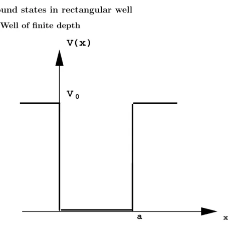
2. ONE DIMENSIONAL RECTANGULAR BARRIERS AND WELLS

Regions of constant potential

In the case of a rectangular potential, V(x) is a constant function V(x) = V in a certain region of the one-dimensional space. In such a region, the Schr¨odinger eq. can be written:

d²

dx²ψ(x) +2m

¯

h² (E−V)ψ(x) = 0 (1)

One can distinguish several cases:

(i) E > V

Let us introduce the positive constant k, defined by k=

p2m(E−V)

¯

h (2)

Then, the solution of eq. (1) can be written:

ψ(x) =Ae^ikx+A^′e^−ikx (3) whereA andA^′ are complex constants.

(ii) E < V

This condition corresponds to segments of the real axis which would be prohibited to any particle from the viewpoint of classical mechanics. In this case, one introduces the positive constantq defined by:

q=

p2m(V −E)

¯

h (4)

and the solution of (1) can be written:

ψ(x) =Be^qx+B^′e^−qx , (5) whereB and B^′ are complex constants.

(iii) E=V

In this special case, ψ(x) is a linear function of x.

The behaviour of ψ(x) at a discontinuity of the potential One might think that at the pointx =x1, where the potential V(x) is discontinuous, the wavefunctionψ(x) behaves in a more strange way, maybe discontinuously for example. This is not so: ψ(x) and ^dψ_dx are continuous, and only the second derivative is discontinuous atx=x1.

General look to the calculations

The procedure to determine the stationary states in rectangular poten- tials is the following: in all regions in whichV(x) is constant we writeψ(x) in any of the two forms (3) or (5) depending on application; next, we join smoothly these functions according to the continuity conditions forψ(x) and

dψ

dx at the points where V(x) is discontinuous.

Examination of several simple cases

Let us make explicite calculations for some simple stationary states according to the proposed method.

The step potential

x V(x)

V

0

I II

Fig. 2.1

a. E > V₀ case; partial reflexion Let us put eq. (2) in the form:

k₁ =

√2mE

¯

h (6)

k₂ =

p2m(E−V₀)

¯

h (7)

The solution of eq. (1) has the form of eq. (3) in the regions I(x <0) andII(x >0):

ψI = A1e^ik1x+A^′₁e^−ik1x ψ_II = A₂e^ik2x+A^′₂e^−ik2x In region I eq. (1) takes the form

ψ^′′(x) + 2mE

¯

h² ψ(x) =ψ^′′(x) +k²ψ(x) = 0 and in the region II:

ψ^′′(x)−2m

¯

h² [V₀−E]φ(x) =ψ^′′(x)−q²ψ(x) = 0

If we limit ourselves to the case of an incident particle ‘coming’ from x =

−∞, we have to chooseA^′₂ = 0 and we can determine the ratiosA^′₁/A₁ and A2/A1. The joining conditions give then:

• ψ_I =ψ_II, at x= 0 :

A₁+A^′₁=A₂ (8)

• ψ_I^′ =ψ^′_II, at x= 0 :

A₁ik₁−A^′₁ik₁ =A₂ik₂ (9) SubstitutingA₁ and A^′₁ from (8) in (9):

A^′₁ = A₂(k₁−k₂)

2k₁ (10)

A₁ = A₂(k₁+k₂) 2k1

(11)

From the two expressions of the constantA₂ in (10) and (11) one gets A^′₁

A₁ = k₁−k₂

k₁+k₂ (12)

and from (11) it follows:

A₂ A1

= 2k₁ k1+k2

. (13)

ψ(x) is a superposition of two waves. The first (the A₁ part) corresponds to an incident wave of momentum p = ¯hk₁, propagating from the left to the right. The second (the A^′₁ part) corresponds to a reflected particle of momentum −¯hk1 propagating in opposite direction. Since we have already chosen A^′₂ = 0, it follows that ψ_II(x) contains a single wave, which is as- sociated to a transmitted particle. (We will show later how it is possible by employing the concept of probability current to define the transmission coefficient T as well as the reflection coefficient R for the step potential).

These coefficients give the probability that a particle coming fromx=−∞

can pass through or get back from the step atx= 0. Thus, we obtain:

R=|A^′₁

A1|² , (14)

whereas forT:

T = k₂ k₁|A₂

A₁|² . (15)

Taking into account (12) and (13) one is led to:

R = 1− 4k₁k₂

(k₁+k₂)² (16)

T = 4k₁k₂

(k₁+k₂)² . (17)

It is easy to check that R+T = 1. It is thus sure that the particle will be either transmitted or reflected. Contrary to the predictions of classical mechanics, the incident particle has a nonzero probability of not going back.

It is also easy to check using (6), (7) and (17), that if E ≫ V0 then T ≃1: when the energy of the particle is sufficently big in comparison with the height of the step, everything happens as if the step does not exist for the particle.

Consider the following natural form of the solution in region I:

ψI =A1e^ik1x+Ae^−ik1x

j=−i¯h

2m(φ^∗▽φ−φ▽φ^∗) (18)

withA₁e^ik1x and its conjugate A^∗₁e^−ik1x: j = −i¯h

2m[(A^∗₁e^−ik1x)(A₁ik₁e^ik1x)−(A₁e^ik1x)(−A^∗₁ik₁e^−ik1x)]

j = ¯hk1

m |A₁|² .

Now with Ae^−ik1x and its conjugate A^∗e^ik1x one is led to:

j=−¯hk₁ m |A|² .

In the following we wish to check the proportion of reflected current with respect to the incident current (or more exactly, we want to check the relative probability that the particle is returned back):

R= |j(φ₋)|

|j(φ₊)| = | − ^¯hk_m¹|A|²|

|^¯hk_m¹|A1|²| =|A

A₁|² . (19)

Similarly, the proportion of transmission with respect to incidence (that is the probability that the particle is transmitted) is, taking now into account the solution in the region II:

T = |^¯hk_m²|A₂|²|

|^¯hk_m¹|A₁|²| = k₂ k₁|A₂

A₁|² . (20)

b. E < V₀ case;total reflection In this case we have:

k₁ =

√2mE

¯

h (21)

q₂ =

p2m(V₀−E)

¯

h (22)

In the regionI(x <0), the solution of eq. (1) [written asψ(x)^′′+k₁²ψ(x) = 0]

has the form given in eq. (3):

ψ_I=A₁e^ik1x+A^′₁e^−ik1x , (23) whereas in the region II(x >0), the same eq. (1) [now written as ψ(x)^′′− q₂²ψ(x) = 0] has the form of eq. (5):

ψ_II =B₂e^q2x+B₂^′e^−q2x . (24) In order that the solution be kept finite whenx→+∞, it is necessary that:

B₂ = 0 . (25)

The joining condition atx= 0 give now:

• ψI =ψII, at x= 0 :

A₁+A^′₁=B₂^′ (26)

• ψ_I^′ =ψ^′_II, at x= 0 :

A1ik1−A^′₁ik1 =−B^′₂q2 . (27) SubstitutingA₁ and A^′₁ from (26) in (27) we get:

A^′₁ = B₂^′(ik1+q2)

2ik₁ (28)

A₁ = B₂^′(ik₁−q₂)

2ik1 . (29)

Equating the expressions for the constantB^′₂ from (28) and (29) leads to:

A^′₁

A₁ = ik₁+q₂

ik₁−q₂ = k₁−iq₂

k₁+iq₂, (30)

so that from (29) we have:

B₂^′

A₁ = 2ik₁

ik₁−q₂ = 2k₁

k₁−iq₂ . (31)