Investigations for the harmonic oscillator

(1)

Isothermal quantum dynamics:

Investigations for the harmonic oscillator

Dem Fachbereich Physik der Universit¨ at Osnabr¨ uck zur Erlangung des Grades eines

Doktors der Naturwissenschaften

vorgelegte Dissertation von Dipl.–Phys. Detlef Mentrup

aus Georgsmarienh¨ utte

Osnabr¨ uck, Januar 2003

(2)

(3)

The key principle of statistical mechanics is as follows:

If a system in equilibrium can be in one of N states, then the probability of the system having energy E_n is (1/Q)e⁻^Eⁿ^/k^B^T, where Q=PN

n=1e⁻^Eⁿ^/k^B^T. (...) If we take |ii as a state with energy E_i and A

∼ as a quantum mechanical operator for a physical observable, then the expected value of the observable is hhA

∼ii = 1/Q P

|iihi|A

∼ |iie⁻^Eⁱ^/k^B^T.

This fundamental law is the summit of statistical mechanics, and the entire subject is either the slide-down from this summit, as the principle is applied to various cases, or the climb-up to where the fundamental law is derived and the concepts of thermal equilibrium and temperature clarified.

R. P. Feynman, Statistical mechanics[1, ch. 1]

(4)

1. Introduction 4

2. Methods of isothermal classical dynamics 9

2.1. The classical Langevin equation . . . 9

2.2. Deterministic temperature control methods . . . 11

2.2.1. The Nos´e-Hoover method . . . 11

2.2.2. The demon method . . . 14

2.2.3. The chain thermostat . . . 16

2.2.4. Non-Hamiltonian phase space as a manifold . . . 18

2.2.5. Note on deterministic chaos and ergodicity . . . 22

3. Coherent states 24 3.1. Introduction . . . 24

3.2. General properties of coherent states . . . 27

3.3. Determination of ensemble averages with coherent states . . . 30

3.3.1. One particle . . . 30

3.3.2. Two identical particles . . . 32

3.3.3. Case ofN fermions . . . 35

4. Isothermal quantum dynamics for the harmonic oscillator 37 4.1. A quantum Langevin equation . . . 37

4.2. The quantum Nos´e-Hoover thermostat . . . 38

4.2.1. One particle . . . 38

4.2.1.1. The Nos´e-Hoover thermostat and the Nos´e-Hoover chain . . . . 38

4.2.1.2. The demon method . . . 40

4.2.2. Two identical particles . . . 41

4.2.2.1. The simple Nos´e-Hoover thermostat . . . 42

4.2.3. Case ofN fermions . . . 45

5. Results 50 5.1. One particle . . . 50

5.1.1. Nos´e-Hoover method . . . 50

5.1.2. Nos´e-Hoover chain method . . . 54

5.1.3. The demon method . . . 56

5.1.4. Convergence speed . . . 57

5.1.5. Mean values of selected observables . . . 58

5.2. Two particles . . . 60

5.2.1. Bose-attraction and Pauli-blocking . . . 60

5.2.2. Ergodicity investigations for two fermions . . . 62

(5)

Contents

5.2.2.1. Nos´e-Hoover method . . . 62

5.2.3. Ergodicity investigations for two bosons . . . 68

5.2.3.1. Nos´e-Hoover method . . . 68

5.2.4. Convergence speed . . . 70

5.2.5. Mean values of typical observables . . . 70

6. Summary and discussion 74

A. The Grilli-Tosatti thermostat 76

B. Position representation of the canonical density operator 80 C. Sinusoidal oscillations of displaced harmonic oscillator eigenfunctions 82

Bibliography 85

Acknowledgements 87

(6)

5.1. Time averaging with a simple Nos´e-Hoover scheme, T = 1 . . . 51

5.2. Time averaging with a simple Nos´e-Hoover scheme, T = 0.25,10 . . . 52

5.3. Time averaging with Nos´e-Hoover chains,T = 0.1 . . . 54

5.4. Short-time behaviour of a Nos´e-Hoover chain dynamics . . . 55

5.5. Time averaging with the cubic coupling scheme, T = 0.2,0.3 . . . 56

5.6. Convergence speed of histograms . . . 58

5.7. Mean values of selected observables . . . 59

5.8. Dynamical illustration of Pauli-blocking . . . 61

5.9. Dynamical illustration of Bose-attraction . . . 61

5.10. Time averaging with a simple Nos´e-Hoover scheme, T = 0.1,1.2 . . . 63

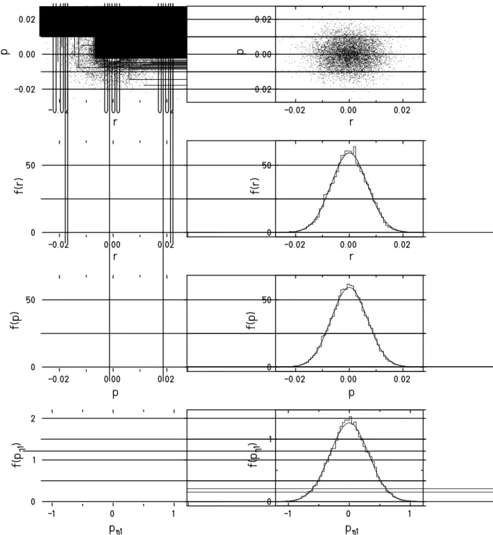
5.11. Density plots and marginal distributions for a Nos´e-Hoover scheme, only one particle is coupled to a thermostat . . . 64

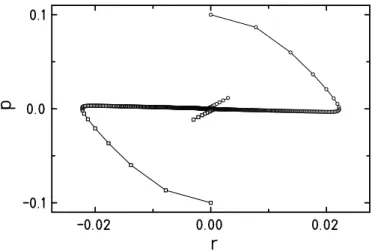
5.12. Short-time behaviour of a Nos´e-Hoover scheme, only one particle is coupled to a thermostat . . . 65

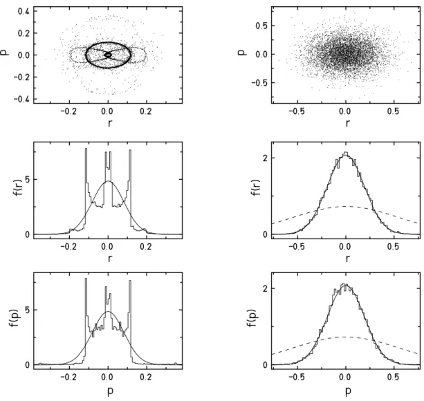
5.13. Marginal distributions for the demon method, fermions . . . 67

5.14. Marginal distributions for the demon method, bosons . . . 69

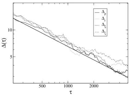
5.15. Convergence speed of histograms, two fermions . . . 70

5.16. Results of time averages for the internal energy and its variance for two fermions 72 5.17. Results of time averages for the two-particle density . . . 73 5.18. Results of time averages for the mean occupation numbers for a two-fermion system 73

(7)

1. Introduction

In a macroscopic system, the number of particles or degrees of freedom is extremely large, such that it is impossible to obtain a complete physical description of the system, both experimentally and theoretically. For example, the microscopic state of a classical gas includes all positions and momenta of ∼10²³ particles. However, the detailed behaviour of the constituents is not reflected on a macroscopic scale, where one is only interested in a few properties of a system, e. g., we only require that a given system has N particles, a volume V and an energy in a small interval around the value E. These macroscopic conditions are met by a large number of microscopic states. The mental collection of systems that are in these states is called an ensemble. The typical problem in statistical physics is the determination of averages over such ensembles.

The three ensembles that are usually dealt with in standard textbooks on statistical physics are the microcanonical (constant number of particles N, volume V, energy E), the canonical (constant N, V, temperature T) and the grand-canonical (constant chemical potential µ, V, T) ensemble. Each of the ensembles is characterised by a distribution function that describes the probability for a macroscopically prepared system to be in a given microscopical state, which is, in classical physics, given by a point in the phase space of the system, whereas in quantum physics it is given by a state vector in Hilbert space. The determination of this distribution function is the fundamental question that is answered by statistical mechanics.

The distribution function permits the calculation of ensemble averages and, more generally, of the partition function, which is of outstanding importance in statistical mechanics since it contains the whole thermodynamics of a system.

Iff(q, p) denotes the classical unnormalised distribution function on the phase space Γ (with configuration coordinates (q₁, . . . q_N) =q and conjugate momenta (p₁, . . . p_N) =p), a classical statistical ensemble average hhBiiof an observable B(q, p) (which in classical mechanics is a function on phase space) is given by the phase space integral

hhB ii= 1 Z_cl

Z

Γ

dqdp B(q, p)f(q, p), (1.1)

i. e. the phase space function corresponding to the macroscopic observable has to be averaged over properly weighted microstates. The quantity

Z_cl = Z

Γ

dqdp f(q, p) , (1.2)

which is used to normalise the above expression, is called the classical partition function.

A direct evaluation of the high-dimensional integrals (1.1) and (1.2) is possible only in very particular cases, such as the ideal gas. In more general cases, e. g. for interacting many-particle systems, it is usually impossible. In order to be able to investigate the wide variety of physically interesting phenomena of these systems, a large number of techniques has been developed for the evaluation of ensemble averages, which can basically be divided into two groups: The stochastic or Monte Carlo methods that make use of random numbers, and the deterministic methods.

(8)

The basic idea of molecular dynamics (MD) simulations is to solve Hamilton’s equations of motion for the particles of a given system numerically to obtain the temporal trajectories q(t), p(t) of all particles in phase space. This is, despite the large number of particles and possibly complicated interactions, usually possible given the availability of both accurate numerical methods and fast computers. Now, in order to calculate an ensemble average, one averages over the time evolution, and hopes that the ergodic hypothesis is satisfied. Loosely speaking, this means that the trajectory runs through the allowed region of phase space¹ with the correct weight such that the average over the time evolution of the system is equivalent to the average over the corresponding statistical ensemble:

τlim→∞

1 τ

Z _τ

0

dt B(q(t), p(t)) = 1 Z_cl

Z

Γ

dqdp B(q, p)f(q, p) . (1.3) In Monte Carlo (MC) methods, one introduces an artificial dynamics on phase space which is based on random numbers. MC simulations are very powerful and popular for static properties.

The most common type of MC simulations, the Metropolis Monte Carlo method [2], is naturally adapted to the canonical ensemble. It allows a direct sampling of the Boltzmann distribution by generating a Markov chain with a suitable transition rule and using rejections to achieve detailed balance. The dynamics obtained in an MC simulation also needs to be ergodic in the sense that the random walk needs to sample the entire allowed phase space such that MC averages and ensemble averages coincide. However, since in MC one does not rely on a

“real” (i. e., physically meaningful) dynamics, this is less of a problem. In case of non-ergodic behaviour, one has to invent more elaborate transition rules.

Usually molecular dynamics calculations are performed with a fixed number of particles in a given volume of constant shape. In addition, as a consequence of Hamilton’s equations, the energy of the system is conserved during time evolution. Therefore, if the trajectory passes uniformly through all parts of phase space that have the specified energy, the time average one obtains from an MD simulation corresponds to a microcanonical ensemble average. Only phase space points which lie on the hypersurface described by the condition of constant energy H(q, p) = E contribute to the equilibrium ensemble average, and they contribute with equal weight according to the principle of equal a priori probability. The corresponding probability density in phase space is therefore given by

f(q, p) =δ(H(q, p)−E) . (1.4)

As a conclusion, the microcanonical ensemble may be considered as the natural ensemble for MD simulations.

However, if this approach to the calculation of ensemble averages were limited to the microcanonical ensemble, it would be practically useless. Experiments are usually carried out at constant temperature (and pressure), and therefore it is desirable to have techniques to realise different types of thermodynamic ensembles in MD simulations. More specifically, in order to obtain a canonical ensemble average, the above technique is inadequate, since in the canonical ensemble, the condition of constant energy is replaced by a condition of constant temperature, and the distribution function (1.4) is replaced by a Boltzmann distribution²,

f(q, p) = exp(−βH(q, p)) . (1.5)

1The term “allowed” refers to the constraints imposed on the system.

2In this work, we will use the notationT for the temperature, andβ= 1/kBTin parallel,kB being Boltzmann’s constant.

(9)

1. Introduction

The total energy of the system is allowed to fluctuate around its mean value by thermal contact with an external heat reservoir which allows for energy exchange. The physical effect of the heat bath upon the system of interest is to impose a constant temperature condition, while the details of the thermal interactions are usually unknown. How can this modified situation be described on the level of the equations of motion, such that the temperature value can be given beforehand as a fixed parameter? Clearly, a mechanism is needed that introduces suitable energy fluctuations. We will call such a mechanism a thermostat.

The constant temperature condition is certainly fulfilled for a Brownian particle which is a macroscopic particle immersed into a liquid of a given temperature. Energy transfer takes place via the ceaseless random collisions between the Brownian particle and the constituents of the liquid. The motion of the particle is described by the so-called Langevin equation, and it has been shown in 1945 that under appropriate conditions, the long-time limit of a time average over the solution of the Langevin equation corresponds to a canonical ensemble average [3].

The Langevin equation involves a stochastic force that mimics directly the collisions mentioned above, therefore we call this approach a stochastic thermostat. In contrast to pure MC sampling, this phenomenological equation is based on Newton’s equation of motion and includes only a

“moderate” amount of randomness.

It is surprising that beyond this direct modelling of the heat bath interaction, a different technique which iscompletely deterministichas been initiated by Nos´e in 1984 [4]. His original method was based on the idea of a scaling of the particle momenta, allowing energy fluctuations and thereby temperature control by a control of the kinetic energy. Although formally correct, the original formulation featured ergodicity problems and therefore was not applied very much in practice. Later on, numerous extensions and refinements have been added that turned out to be more efficient and easier to handle. These modified techniques are known as extended system methods. Their common underlying idea is to append additional degrees of freedom to the original physical system that act as pseudofriction terms, thereby destroying energy conservation and, moreover, the overall Hamiltonian structure of the dynamics. The equations of motion of the enlarged system are designed in such a way that in the subspace belonging to the original physical system, the temporal average corresponds to a canonical average. To ensure this, the equipartition theorem of classical statistical mechanics is implicitly exploited.

Extended system methods are commonly used nowadays in classical MD simulations [5, 6] and have turned out to be extremely powerful.

The main advantage a molecular dynamics approach has over Monte Carlo is that in the course of an MD simulation, physically reasonable dynamical equations are integrated. This makes dynamical information available, even though one can argue that the particular constant temperature methods appear somewhat artificial. Consequently, dynamical properties such as time correlation functions may be calculated. Monte Carlo simulations are not suitable for the determination of dynamical physical properties and allow only the calculation of static properties, unless one accepts that the random walk generated by MC is an interesting physical dynamical model.

In the field of finite-temperature simulations of quantum systems, the most successful approach is based on the path-integral formulation by Feynman [1]. The power of the method is due to the fact that it allows to relate the quantum density matrix at arbitrary temperature, e⁻^βH^∼, whereH

∼ is the Hamiltonian of the system, to integrals over paths in coordinate space, hR| e⁻^βH^∼ |R⁰i=

Z

· · · Z

dR₁. . .dR_M exp(−S(R₁, . . . R_M)). (1.6) S is the so-called action of the path and is real, and thus (1.6) involves a basically classical

(10)

interacting boson system ⁴He that undergoes the famous λ-transition at T = 2.18K [8], and to bosons in a magnetic trap [9]. However, for fermions, the contributions of even and odd permutations to the density matrix involve opposite signs due to the required antisymmetry of the wave function. The cancellation of contributions usually causes the signal/noise ratio to approach zero rapidly and rules out a straightforward MC evaluation of the integrand. This is known as the “fermion sign problem”.

The main obstacle to an approach to the calculation of ensemble averages via time averaging over the quantum time development is the fact that the solution of the Schr¨odinger equation is notreadily available for complicated systems. Contrary to the classical case, quantum dynamics itself is a very hard computational problem. In essence, the quantum time evolution implies to calculate an exponential of the Hamiltonian, which is practically equivalent to treating the canonical density operator directly. On this level, the ansatz of time averaging does not lead to substantial computational advantages. Nevertheless, the question whether it is possible to determine canonical averages for a quantum system by averaging over trajectories generated by an appropriate dynamics is challenging.

The interest for techniques comparable to the classical extended system methods in the realm of finite-temperature quantum MD simulations has different sources. On the one hand, even for relatively simple quantum systems constisting of a very small number of particles, it is usually impossible to determine the full set of eigenfunctions and eigenvalues. Given the availability of various efficient approximate quantum MD schemes (for a review of techniques for fermions, see [10]), the following question is interesting from a methodological point of view: Does a generalisation of the classical methods to quantum dynamics permit to make the power of approximate quantum MD schemes available for the calculation of equilibrium averages without diagonalising the full many-body Hamiltonian? The present work may be considered a first step towards an affirmative answer to this demanding question. Beyond, given the fact that quantum MC has a non-physical time evolution, it is highly desirable to have an isothermal quantum MD method at hand that depicts the physical dynamics of the system at a given finite temperature more realistically. This would enlarge the variety of techniques available in many-body theory and possibly extend their overall range of applicability.

Apart from permitting the determination of equilibrium ensemble averages, the classical extended system methods also offer a model scenario for the dynamical evolution of a non- equilibrium state towards thermal equilibrium. Although it is not clear whether the specific approach using pseudofriction terms is a faithful physical picture of the real dynamical evolution of a system enroute to thermal equilibrium, this view is a natural interpretation of the methods that permit “cooling” and “heating” of non-equilibrium initial states. Consequently, one may hope that a quantum analogue of the classical methods models the approach of a quantum system to equilibrium.

On the other hand, real physical systems such as ultracold trapped gases are in the focus of modern research for which such a method appears to be tailor-made and may allow for the direct theoretical analysis of systems in a constant temperature condition. Recently, investigations of ultracold magnetically trapped atomic gases have led to the discovery of intriguing physical phenomena, among them the spectacular evidence for Bose-Einstein condensation in weakly interacting Bose gases [11, 12]. On the fermionic side, researchers study the large impact of Fermi-Dirac statistics on the behaviour of so-called degenerate Fermi gases [13, 14]. It is remarkable that these systems constitute dilute gases in which the interparticle interactions are weak. For fermions, the quantum statistical suppression of s-wave interactions makes an

(11)

1. Introduction

ultracold trapped gas of fermionic atoms even an excellent realisation of an ideal gas. In addition, we note that the confinement by the magnetical trap may approximately be considered as harmonic [15]. Beyond, from a theorist’s point of view, the ideal gas forms the starting point for perturbative treatments of interacting many-particle assemblies, and motion in a common harmonic oscillator potential is of special interest because of its importance for low- excitation dynamics. Therefore, it appears reasonable to start with this tractable case. In interacting fermion systems, a number of other fascinating effects is discussed, e. g., theorists have studied the prospects of observing a superfluid phase based on the BCS concept of Cooper- pair formation [16].

First ideas for a translation of classical constant temperature MD methods to quantum mechanics have been discussed by Grilli and Tosatti in 1989 [17], but their approach has turned out to have serious shortcomings [18] some of which are discussed in appendix A. An alternate method due to Kusnezov [19] is limited to quantum systems of finite dimensionality and has only been applied to a two-level system. Schnack has investigated a quantum system at constant temperature using a thermometer and a feedback mechanism to drive the system to the desired temperature value by complex time steps [20]. The main drawback of this ansatz is the fact that an interaction is needed to equilibrate the system of interest and the thermometer, which leads to a perturbation of the original system and thereby excludes simulations at very low temperatures. This illustrates a main difficulty encountered in quantum mechanics: While in classical mechanics, the equipartition theorem provides a direct and infallible “thermometer”, such a useful a priori relation between the average value of some observable and temperature is not readily at hand in quantum mechanics. Instead, it needs to be implemented in a sophis- ticated manner, involving a number of difficulties, like the perturbation due to the interaction and the insecurity about correct equilibration between system and thermometer.

In view of this unsatisfactory situation, the major goal of the present work has been to de- vise a quantum thermostat following the lines of the methods successfully employed in classical mechanics. We will show that in the case of an ideal quantum gas enclosed in an external harmonic oscillator potential, the framework of coherent states permits new, far-reaching methodological developments. For a single quantum particle, the analogy to classical physics is very close, whereas for two non-interacting indistinguishable quantum particles genuine quantum features have been found and investigated. It turns out that the approach based on the classical Langevin equation is not suitable for identical particles, whereas the extended system methods can successfully be translated to quantum mechanics.

The outline of the present work is as follows. Chapter 2 deals with temperature control methods in classical mechanics, namely the Langevin equation and the extended system method of Nos´e and Hoover along with its refinements. Chapter 3 gives a brief introduction to coherent states and their properties. Chapter 4 contains the main outcome of this work, presenting the unprecedented quantum thermostat methods for one and two particles, and N fermions in an external harmonic oscillator potential. In chapter 5, the results obtained with the new methods are presented. Chapter 6 summarises the work and gives a critical analysis of the chances and limits of the quantum thermostat method devised in this work.

(12)

2.1. Stochastic temperature control:

The classical Langevin equation

The Langevin equation may be regarded as a phenomenological approach to temperature control in classical mechanics. It has been developed to describe the irregular motion of a macrosopic (so-calledBrownian) particle immersed into a liquid of absolute temperatureT. The main idea is to describe the action of the liquid that acts as a heat bath upon the particle by two additional forces that are introduced in Newton’s equation of motion: Firstly, a slowly varying frictional force proportional to the velocity of the particle, −mγ _dt^dq, wherem is the mass of the particle and γ is a constant frictional coefficient, and secondly, a rapidly fluctuating random forceF(t) that describes the disordered collisions of the particles of the liquid with the Brownian particle and that vanishes on average. If in addition the particle moves in an external potential V(q), the resulting equation describing its motion on the spatial q-axis reads

md²q

dt² =−∂V

∂q −mγdq

dt +F(t) . (2.1)

Equivalently, one can study the set of equations of first order in time, dq

dt = p

m , dp

dt =−∂V

∂q −γ p+F(t) . (2.2)

The time average of F(t) vanishes,

τlim→∞

1 τ

Z τ 0

F(t)dt= 0 , (2.3)

andF(t) shall be purely random, which means that it has a vanishingly short correlation time¹. Moreover, the amplitude of the random force is related to the temperature T and the friction coefficient γ by the second fluctuation-dissipation theorem, which together is expressed as

hhF(t₁)F(t₂)ii= 2mγk_BT δ(t₁−t₂) . (2.4) In addition, for technical reasons, one must assume that the random force is Gaussian, i. e. one assumes that the coefficients of the Fourier series of F(t) (which are random variables) are distributed according to a Gaussian distribution.

Equation (2.4) guarantees that the temperature is kept at a constant value by the balance between the thermal agitation due to the random force and the slowing down due to the friction.

Under the assumptions made above, it has been shown that in the limitt→ ∞, the probability densityP(q, p;t|q₀, p₀) at the phase space point (q, p) given that at timet= 0 the particle was

1As a result of the Wiener-Khintchine-theorem that relates the correlation function of a stochastic function to its power spectrum [21], the spectral density of the fluctuating force is constant under this condition.

Therefore, the spectrum ofF(t) is frequently said to bewhite.

(13)

2. Methods of isothermal classical dynamics

situated atq₀ with initial momentump₀ is the canonical Maxwell-Boltzmann density [3]. This limiting probability distribution is independent of the initial state of the system. Therefore, a time average over a sufficiently long period will be equivalent to a canonical ensemble average.

The proof that the limiting probability distribution of the Langevin equation (2.1) is a Maxwell-Boltzmann distribution uses a Fokker-Planck equation associated to (2.1) [3, 21]. In general, for a one-dimensional Markov process y(t), the Fokker-Planck equation is a partial differential equation for the probability density P(y, t|y₀) that is derived from the obvious condition

P(y, t+ ∆t|y₀) = Z

dz P(y,∆t|z)P(z, t|y₀) , (2.5) which is called the Smoluchowski equation, in the limit of small ∆tand a small differencey−y0. The resulting Fokker-Planck equation for a one-dimensional Markov process,

∂P

∂t =− ∂

∂y(M₁(y)P) + 1 2

∂²

∂y²(M₂(y)P) , (2.6)

contains the first and second moment of the change of the random variabley, thenth moment being defined as

Mn(y) = lim

∆t→0

1

∆t Z

dz(z−y)ⁿP(z,∆t|y) . (2.7) Equation (2.6) is derived assuming that the momentsM_n vanish forn >2 which expresses the fact that in a short period of time, the spatial coordinate can only change by small amounts.

The Fokker-Planck equation for ann-dimensional Markov process y= (y1, . . . , yn) reads

∂P

∂t =− Xn

i=1

∂

∂y_i(M₁(y)P) + 1 2

Xn k,l=1

∂²

∂y_k∂y_l(M_2kl(y)P) . (2.8) The case of the harmonic oscillator, V(q) = ¹₂mω²q², is particularly simple. The moments required in the Fokker-Planck equation can be determined, and the resulting equation for the probability density P(q, p;t) reads explicitly

∂P

∂t =−p m

∂P

∂q + ∂

∂p

γ p+mω²q P

+mγkBT ∂²P

∂p² (2.9)

and may be solved analytically with the initial conditions

P(q, p, t= 0) =δ(q−q0)δ(p−p0) . (2.10) The result is a two-dimensional Gaussian distribution inq and p with time-dependent average values and widths. In the limitt→ ∞, one obtains the Maxwell-Boltzmann distribution (C is a normalisation constant),

tlim→∞P(q, p;t|q₀, p₀) =Cexp

− 1 k_BT

p² 2m+ 1

2mω²q²

, (2.11)

which is a Gaussian distribution both in positions and momenta, independent of the initial conditions. Note that the amplitude of the random force (2.4) which contains the temperature T determines the width of the limiting Gaussian distribution.

(14)

We summarise the main points of this section. The long-time limit of a time average over the solution of the classical Langevin equation corresponds to a canonical ensemble average. In the simplest case of the harmonic oscillator, the solution of the Langevin equation provides an average with Gaussian distribution functions. This statement is verified by an explicit solution of the associated Fokker-Planck equation. The width of the Gaussians is determined by the amplitude of the fluctuating force via the fluctuation-dissipation relation.

2.2. Deterministic temperature control methods

While the Langevin approach is readily comprehensible and physically intuitive, it is less evident that acompletely deterministictime development may also provide canonical averages. Such an alternate technique has originally been proposed by Nos´e [4], and has been refined by Hoover [22], Kusnezov, Bulgac, and Bauer [23], and Martyna, Klein, and Tuckerman [24]. A review of these and various other constant temperature molecular dynamics methods can be found in [25]. Only recently [26], the theory of these methods was put on a firm theoretical ground, providing a valuable deeper view that we present in section 2.2.4.

In the original method of Nos´e, temperature control in a molecular dynamics simulation is achieved by the introduction of an additional degree of freedomsthat is used to scale time and thereby the particle velocities. This is reasonable since temperature is related to the average of the kinetic energy. However, Nos´e’s original formulation, although formally correct, features substantial problems in practice, and therefore, the method has been modified and refined.

The so-called classical Nos´e-Hoover thermostat with the extension to chains of thermostats and the so-called demon method have turned out to be most successful and reliable. Simply speaking, these methods exploit the equipartition theorem to determine the equations of motion of pseudofriction coefficients that are introduced in the equations of motion of the original system. These methods may be transferred to the quantum harmonic oscillator, which is why the functionality of these classical deterministic thermostats is the subject of the following paragraphs and will be outlined in detail.

2.2.1. The Nos´e-Hoover method

Consider an isolated classical N-particle system in one dimension described by a Hamiltonian, H(q, p) =

XN i=1

p²_i

2m +V(q) . (2.12)

As usual, the ith particle is located at position qi with momentum pi, and q (resp. p) is the N-tuple of all positions (momenta). The motion of the system in phase space is governed by Hamilton’s equations,

d

dt q_i= ∂H

∂p_i = p_i

m , d

dt p_i=−∂H

∂q_i =−∂V(q)

∂q_i . (2.13)

In the Nos´e-Hoover method, the equations of motion of the momenta p_i are supplemented by a term similar to a frictional force. In order to permit energy fluctuations, the frictional coefficient is regarded as time-dependent and can assume both positive and negative values. In contrast to the Langevin approach, a stochastic force is not employed. One wants to obtain canonical time averages solely from varying the frictional coefficient suitably in time.

(15)

In the original notation introduced by Hoover [22], the modified equations of motion read d

dt q_i= p_i

m , d

dt p_i=−∂V(q)

∂q_i −ζ(t)p_i , (2.14)

whereζ(t) is a time-dependent supplementary degree of freedom added to the system to drive the energy fluctuations required in the canonical ensemble. Therefore, the Nos´e-Hoover and related methods are frequently referred to asextended system methods.

From (2.14) it can be inferred thatζ acts as a pseudofriction coefficient. Both the value and the sign ofζ vary in time. Accordingly, the momenta of the original system either decrease or increase, which leads to a change of the kinetic energy of the system. This mechanism is used for temperature control. The key point is to determine the time dependence ofζ such that the energy fluctuations correspond to the canonical ensemble. More precisely, we demand that the weight with which the phase space of the original system is sampled in time is the canonical distribution function,

exp −βH(q, p)

. (2.15)

On the level of the phase space of the extended system we postulate the distribution function f(q, p, ζ) = exp

−β

H(q, p) +1

2Qζ²

. (2.16)

Note that the Boltzmann distribution (2.15) is a marginal off. The choice of the distribution function forζis related to the linear coupling−ζpiin the equation of motion (2.14). A different coupling would entail a different distribution function, as will become evident in the discussion of the demon method.

In order to make sure that f is sampled during time evolution, the time dependence ofζ is determined by the condition thatf is the stationary solution of a generalised Liouville equation which we derive now. To fix the notation, let x denote a point in a (possibly enlarged) phase space. A distribution function f(x) satisfies a continuity equation that expresses conservation of probability,

∂f

∂t + div_x(fx) = 0˙ . (2.17)

This equation is obtained by equating the local change of a conserved quantity inside a given volume and the flow of this quantity through the surface of this volume. On the other hand, the total time derivative of f along a phase space trajectory is defined by

d

dt f = ∂f

∂t + ˙x· ∂f

∂x . (2.18)

With this identity, (2.17) can be reexpressed as d

dt f =−f ∂

∂x ·x˙

. (2.19)

Note the modified notation divxx˙ ≡ _∂x^∂ ·x.˙

Now, if x = (q, p) is an element of the phase space of a Hamiltonian system and the time evolution of the system is determined by Hamilton’s equations of motion (2.13), the right hand side of this equation vanishes identically and Liouville’s theoremdf /dt= 0 holds. Its meaning

(16)

is that given an initial distribution in phase space, the local density of representative points does not change if we follow the solution of Hamilton’s equations.

In the case of the Nos´e-Hoover equations (2.14) on the enlarged phase space, i. e. with x= (q, p, ζ), we use this equation to determine an equation of motion for ζ so as to reproduce the postulated thermal distribution (2.16). In order to obtain an explicit equation, we impose the constraint ∂ζ/∂ζ˙ = 0, and along with (2.14) we easily get for the right hand side of (2.19)

−f ∂x˙

∂x

=−f XN i=1

∂

∂qi

˙ q_i+ ∂

∂pi

˙ p_i

+ ∂

∂ζζ˙

!

=f N ζ . (2.20) Now, we calculate the left hand side of (2.19), employing the equations of motion (2.14),

d

dt f = ∂f

∂pp˙+∂f

∂qq˙+∂f

∂ζζ˙ (2.21)

=f · −β XN

i=1

p_i

mp˙_i+∂V

∂q_iq˙_i

−βQζζ˙

!

=f β ζ· XN i=1

p²_i m −Qζ˙

! .

Equating (2.20) and (2.21) yields the following equation of motion for ζ:

d

dt ζ = 1 Q

XN i=1

p²_i

m −N kBT

!

. (2.22)

It is interesting to notice that the time evolution ofζ is determined by the deviation of the momentary value of the kinetic energy P

ip²_i/2m from its canonical average value N/2 kBT. As a result, temperature control is achieved by a feedback mechanism: In case the momentary kinetic energy is larger than N/2 k_BT, the time derivative of ζ is positive and ζ increases, so that the frictional force −ζpi reduces the momenta, thereby “cooling” the system. In the opposite case, the feedback mechanism heats the system up by accelerating the particles.

Besides, it is noteworthy that the influence of a heat bath may be imitated by adding a single supplementary degree of freedom to the original system. This is in striking contrast to the usual attributes of a heat bath, namely, that it is “larger” in comparison to the system of interest, which is usually exposed as “having much more degrees of freedom” [21, ch. 3.6].

Furthermore, we remark that in the Nos´e-Hoover method, the canonical distribution in phase space is reproduced from a single thermodynamic average, the average of the kinetic energy.

For reasons of completeness, the following equation d

dt Θ =ζ (2.23)

is also solved in a simulation, since it contributes to the quantity H⁰ =H(q, p) +1

2Qζ²+N k_BTΘ (2.24)

that is conserved by the set of equations of motion (2.14) and (2.22). We stress that the quantity (2.24) is not a Hamiltonian for the extended system; the equations of motion (2.14), (2.22) along with (2.23) do not have a Hamiltonian form. This is the reason why we considered

(17)

the non-Hamiltonian phase space (q, p, ζ) of odd dimensionality. We have abandoned the strict Hamiltonian structure in the present context. The question of a sound generalisation of the Hamiltonian phase space notions to a non-Hamiltonian system will be addressed more closely in section 2.2.4.

By construction, f is the static probability distribution generated by the dynamics (2.14) and (2.22). This condition is necessary, but not sufficient for the equivalence of a trajectory average and an ensemble average. It does not guarantee that the correct limiting distribution will be generated by the dynamics, since it is not clear whether the system actually runs through all phase space points with the correct weight, independent of the initial conditions.

In fact, it might be possible that some regions of phase space are unreachable for the dynamics and therefore not sampled. Loosely speaking, the many body system needs to be sufficiently complex such that the dynamics will cover the entire phase space. The analysis by Tuckerman et al. presented in section 2.2.4 allows to expose this point very clearly.

This additional property, the equivalence of time average and ensemble average, is generally referred to as ergodicity. A strict proof of ergodic behaviour for a given system can rarely be given, however, it is observed that the more complex the dynamics of a system gets, the more likely ergodic behaviour is observed. This is intuitively understandable since it is clear that the number of unwanted conserved quantities decreases with increasing complexity. When using deterministic methods such as the Nos´e-Hoover method, one usually checks the marginals of the additional degrees of freedom and hopes that if these marginals are sampled correctly, the phase space of the entire system is also sampled correctly [6].

There is an important example of apparent non-ergodic behaviour in the case of the Nosé- Hoover method. The classical harmonic oscillator cannot be thermalised by the simple scheme outlined above [22]. The shape of the Poincaré-sections in phase space strongly depends on the choice of the numerical value ofQ, and the distributions sampled do in no case correspond to a canonical distribution. For other systems, among them classical spin systems, it was found that the simple Nosé-Hoover scheme may be ergodic for one temperature, but not ergodic for a different value of T [23, 6]. In addition, in all cases of non-ergodic behaviour, a strong dependence of the initial conditions is observed, which is unacceptable. In summary, the Nosé- Hoover method is not capable to reliably create canonical distributions.

However, more general schemes like the demon method or the method of chain thermostats basically resolve this problem by generating a more complex dynamics. A deeper study using the notions of section 2.2.4 sheds light on the problem underlying the non-ergodicity of the harmonic oscillator.

2.2.2. The demon method

In an effort to cure the problem of unpredictable non-ergodic behaviour in the Nos´e-Hoover method, Kusnezov, Bulgac, and Bauer [23] have devised a generalised coupling scheme. Two additional degrees of freedom are used to replicate the interaction of the original system with a heat bath. The first one is coupled to the equations of motion of the positions, the second one to the momenta of the particles. This approach appears sensible since it takes into account the equality of positions and momenta in Hamiltonian mechanics. Another advantage of this method is that the Hamilton function of the envisaged system does not have to contain a kinetic energy term for temperature control; instead, the time derivative of the pseudofriction coefficients turns out to be proportional to the difference of two quantities whose ratio of canonical averages is k_BT. This extends the range of applicability of the method to, e. g., classical spin systems [27, 6].

(18)

Explicitly, the equations of motion of the KBB-scheme read d

dt q_i= ∂H

∂p_i −g⁰₂(ξ)F_i(q, p) , d

dt p_i =−∂H

∂q_i −g⁰₁(ζ)G_i(q, p) . (2.25) The additional degrees of freedom ζ and ξ are frequently referred to as demons which are coupled to the equations of motion with the functions g⁰₁(ζ) and g₂⁰(ξ). F_i(q, p) and G_i(q, p) are arbitrary functions of all coordinates and momenta. Note that the original Nos´e-Hoover equations are obtained from (2.25) by the specific choice G_i =p_i, g₁⁰ =ζ, andF_i =g⁰₂= 0.

The phase space distribution function in the (2N+2)-dimensional extended phase space is chosen to be

f(q, p, ζ, ξ) =Cexp

−β

H(q, p) + 1 κ1

g₁(ζ) + 1 κ2

g₂(ξ)

, (2.26)

whereC is again a normalisation constant, andκ1 andκ2 are, at the moment, free parameters.

The functions g₁ and g₂ that determine the thermal distribution of the demons need to be chosen such that the integral off with respect toζ andξ converges. Note that their respective derivatives g₁⁰, g⁰₂ appear in the equations of motion (2.25). This has been the reason for choosing a Gaussian distribution function forζ in (2.16).

In order to derive equations of motion forζ andξso as to reproduce the postulated thermal distribution (2.26), we substitute the equations of motion (2.25) and the distribution function f into the generalised Liouville equation (2.19) derived in the preceding section. In addition, we have the freedom to impose the constraints

∂ζ˙

∂ζ = 0 , ∂ξ˙

∂ξ = 0 . (2.27)

By comparing the coefficients of the functions g⁰₁, g₂⁰ in the generalised Liouville equation, one obtains the following equations of motion for the demons:

d

dt ζ =κ1

XN i=1

∂H

∂p_iGi− 1 β

∂G_i

∂p_i

, (2.28)

d

dt ξ=κ₂ XN i=1

∂H

∂q_iF_i− 1 β

∂F_i

∂q_i

.

The equations of motion (2.25) and (2.28) conserve the quantity H⁰ =H(q, p) + 1

κ1

g₁(ζ) + 1 κ2

g₂(ξ) + 1 β

Z t

dt⁰ X

i

g₁⁰(ζ(t⁰))∂G_i

∂pi

+g₂⁰(ξ(t⁰))∂F_i

∂qi

. (2.29) By partial integration, one easily shows that

k_BT hh ∂G_i

∂pi ii=hh ∂H

∂pi

G_i ii, (2.30)

and likewise

k_BT hh ∂F_i

∂q_i ii=hh ∂H

∂q_iF_i ii. (2.31)

(19)

In fact, the time dependence of the demons is determined by the difference of two quantities whose ratio of canonical averages is k_BT. The control of the kinetic energy in the original Nos´e-Hoover thermostat is only a special case. This paves a way for the generalisation of this method to systems whose Hamiltonian does not contain a kinetic energy term. As an example, we mention classical spin systems, where this method has been employed successfully for extensive studies [27, 6].

In principle, since the choice of the functions F, G, g₁, g₂ is arbitrary, this method offers a lot of freedom. Kusnezov, Bulgac, and Bauer have investigated different choices of the various functions and were able to show that the demon method frequently resolves problems of non- ergodic behaviour. The most prominent choice of functions is the following so-called cubic coupling scheme:

g₁ = 1

4ζ⁴ , g₂= 1

2ξ² , F_i =q³_i , G_i =p_i , (2.32) resulting in the set of equations of motion

d

dt q_i= p_i

m −ξq³_i , d

dt p_i=−∂V

∂q_i −ζ³p_i , (2.33) d

dtζ =κ₁ XN i=1

p²_i

m −N k_BT

! , d

dtξ=κ₂ XN i=1

∂V

∂q_iq³_i −3k_BT XN i=1

q²_i

! .

These equations provide ergodic behaviour in all examples given in [23], see also section 2.2.5.

The problems of the simple Nos´e-Hoover scheme – dependence of the choices ofQ, T, and the initial conditions – are reliably resolved. The choice of the numerical values ofκ₁ and κ₂ may still influence ergodicity, but rules of thumb have been found empirically that will be discussed in chapter 5.

2.2.3. The chain thermostat

Another variation of the Nos´e-Hoover method has been proposed by Martyna, Klein, and Tuckerman [24]. The main idea of this technique is to impose on the first thermalising pseudofriction coefficient a second one which may be coupled to yet a third one, and so on, thereby forming a chain of thermostats. This approach of recursive thermalisation increases the size of the phase space and thus makes the dynamical evolution of the system more complex, thereby leading to ergodicity.

In a modified notation (ζ ≡p_η/Q), the set of dynamical equations d

dt q_i= p_i

m , d

dt p_i=−∂V(q)

∂q_i −p_ip_η

Q , (2.34)

d dt p_η =

XN i=1

p²_i

m −N k_BT , d

dt η= p_η Q ,

defines Nos´e-Hoover dynamics. The fact that the temporal evolution ofp_η is governed by the deviation of the kinetic energy of the system from its canonical average value is displayed very

(20)

obviously. The variable ηwhich is not coupled to the dynamics is again included for reasons of completeness. The stationary distribution function reads

f(q, p, p_η) = exp −β

H(q, p) + p²_η 2Q

!

, (2.35)

and the conserved quantity is

H⁰(q, p, pη, η) =H(q, p) + p²_η

2Q +N kBT η . (2.36) The desired distribution (2.35) has a Gaussian dependence on the particle momenta as well as on the thermostat momentum p_η. While the Gaussian fluctuations of the particle momenta are driven by p_η, there is nothing to equilibrate p_η itself. Therefore, it appears sensible to couple another pseudofriction coefficient to the first one, and so on. As a result, one obtains the equations of motion of the Nos´e-Hoover chain method,

d

dt q_i = p_i

m , d

dt p_i =−∂V(q)

∂q_i −p_ip_η₁

Q₁ , (2.37)

d dt p_η₁ =

XN i=1

p²_i

m −N k_BT

!

−p_η₁pη2

Q₂ , d

dt pηj = p²_η_j−1

Q_j₋₁ −kBT

!

−pηj

p_η_j+1 Q_j+1 , d

dt p_η_M = p²_η_M₋₁

QM−1 −k_BT , d

dt η_i = pηi

Q_i ,

where a chain of M thermostats has been implemented. These equations have the stationary phase space distribution

f(q, p, pη) =Cexp



−β

H(q, p) + XM j=1

p²_η_j 2Q_j



 (2.38)

and the conserved quantity

H⁰(q, p, η_j, p_η_j) =H(q, p) + XM j=1

p²_η_j

2Q_j +N k_BT η₁+k_BT XM j=2

η_j . (2.39)

Although the number of degrees of freedom added in this approach is usually larger than in the demon method, the addition of the successive thermostats is numerically inexpensive as they form a simple one-dimensional chain. Only the first thermostat interacts with allN particles. A thorough analysis of the method has shown that it reliably leads to ergodicity, see section 2.2.5, and that it is competitive with the demon method with regard to the speed of convergence.

(21)

2.2.4. Non-Hamiltonian phase space as a manifold

Tuckerman, Mundy, and Martyna have pointed out that all derivations outlined above do not properly take into account that the equations of motion such as (2.14) along with (2.22), (2.33), or (2.37) describe non-Hamiltonian systems. In [26], a consistent classical statistical mechanical theory for such systems is presented. It is based on the concepts of differential geometry as applied to dynamical systems and provides a sound generalisation of the usual Hamiltonian based statistical mechanical phase space principles to non-Hamiltonian systems.

Using these notions, a procedure is developed that leads to the phase space counterpart of the time averages generated by a non-Hamiltonian system. Besides, this approach reveals and surmounts a number of weaknesses of the original formulation, e. g., it permits to explore the reason for the apparent non-ergodicity of certain systems, notably the classical harmonic oscillator [28].

We shall briefly outline the basic ideas presented in [26]. Traditional classical statistical mechanics is based on a Hamiltonian function. A point in the phase space of a system is given by the coordinates and momenta x= (q, p). Given a time-dependent phase space distribution functionf(x, t), the average of an observable B(x) in the ensemble described byf is given by

hhBii(t) =

R dⁿx B(x)f(x, t)

R dⁿx f(x, t) . (2.40)

The measure dqdp ≡ dⁿx, which is used for the calculation of phase space averages, is preserved by Hamiltonian dynamics. This means that a subset of systems with initial conditions contained in a phase space volume element dⁿx₀ will at a later time occupy a volume element of the same size²: dⁿx₀ = dⁿx_t. This property of Hamiltonian dynamics is frequently referred to as the incompressibility of phase space flow. It is tantamount to the statement that the coordinate transformation specified by the solution of Hamilton’s equations of motionx_t(t;x₀) has a Jacobian of absolute value 1. The existance of this time-invariant measure implies that (2.40) can be computed with respect to the phase space variablesx at any timet.

In the case of a general non-Hamiltonian dynamical system,

˙

x=ξ(x, t) , (2.41)

the situation becomes more complicated. The time evolution generated by the set of differential equations (2.41) is in general compressible and the usual phase space measure dⁿxis no longer invariant under the dynamical evolution. Therefore, in a more refined analysis of the situation, one must treat the phase space of the system as a general Riemannian manifold. The metric on this manifold has to be taken into account in the formulation of a continuity equation for the distribution function and in the expression of a phase space average which is given in terms of an integral over the manifold.

Moreover, if one wants to relate a phase space average to a time average, the question of the integration measure needs to be considered carefully. Analogous to the Hamiltonian case, an expression for an ensemble average is needed that uses a measure on phase space that is invariant under time evolution. If such aninvariant measureis found, the phase space average of some property (expressed in terms of an integral over the manifold with the preserved measure) corresponds to the time average of the same property over the trajectories of the system under the usual assumption of ergodicity.

2Together with the statement that trajectories of identical systems do not intersect (since the solution of Hamilton’s equations of motion is unique), one easily proves the theorem of Liouville, _dt^d f= 0.

(22)

In order to derive an invariant measure on this manifold, consider the solution of (2.41), xⁱ_t =xⁱ_t(t;x¹₀, . . . xⁿ₀) , i= 1, . . . n , (2.42) as a coordinate transformation from the initial coordinates at time t= 0 to the coordinates at time t. It can be shown that the Jacobian J(x_t;x₀) of this transformation,

J(x_t;x₀) = det∂(x¹_t, . . . xⁿ_t)

∂(x¹₀, . . . xⁿ₀) (2.43) obeys the equation of motion

d

dt J =Jκ(xt) , (2.44)

where the quantity κ(x_t) = Pn

i=1∂x˙ⁱ/∂xⁱ is called the phase space compressibility of the dynamical system³. Since equation (2.44) may be rewritten as

d

dt lnJ =κ , (2.45)

it can be integrated easily. If we introduce the variable w(x) related toκby ˙w=κ, the solution reads

J(x_t;x₀) = exp w(x_t)−w(x₀)

. (2.46)

The infinitesimal volume element transforms under a coordinate transformation according to dⁿx_t =J(x_t;x₀)dⁿx₀ . (2.47) Rearranging this equation such that quantities at time t appear on one side and quantities at t= 0 appear on the other, we get

e⁻^w(x^t⁾dⁿx_t =e⁻^w(x⁰⁾dⁿx₀ . (2.48) This equation shows that the measure e⁻^w(x^t⁾dⁿx_t is conserved by the dynamics. The metric determinant of the transformation can be identified as √g= exp(−w(x)). Due to the general transformation law of the metric tensor, it is clear that the values of √g at times 0 and t are related by the Jacobian,

√g₀ =√

g_tJ(x_t;x₀) . (2.49)

Consequently, √gsatisfies the following differential equation, d

dt

√g=−√g κ . (2.50)

Note that the same equation is fulfilled by the inverse J⁻¹ of the Jacobian J as can easily be seen from equation (2.44) and the relation J J⁻¹ = 1.

Next, if an ensemble of systems on phase space is considered, a continuity equation that accounts for number conservation must be expressed. It may be regarded as a generalisation of the theorem of Liouville. The change of local density is balanced by a flux through the

3This same quantity already occured on the right hand side of (2.19)

(23)

boundary surface taking into account the geometry of the space. As a result, the following equation is obtained [26]:

∂(f√g)

∂t +∇ ·(f√gx) = 0˙ . (2.51) This equation can be put into the form of equation (2.17) by defining a new function ˜f =√gf, but such an identification is not general, since it entails problems with a coherent notion of the entropy of a system [26]. Finally, note that equations (2.50) and (2.51) together imply that even in the case of a non-Hamiltonian system,f(x, t) is conserved,

d

dt f = 0 . (2.52)

The notion of ergodicity may now be exposed more clearly. Suppose that the set of dynamical equations (2.41) possesses a set ofn_c conserved quantities Λ_k(x), k = 1, . . . n_c, satisfying

d

dt Λ_k= 0 . (2.53)

As a consequence, the trajectories generated by equation (2.41) will only sample the intersection of the hypersurfaces {Λ_k(x) = C_k}, where C_k is a set of constants. If all points on a given hypersurface have the same probability of being visited by a trajectory, then the system is said to be ergodic. In this case, a time average corresponds to a microcanonical average of the extended system which is a phase space average with the distribution function

f(x) =

nc

Y

k=1

δ(Λ_k−C_k) , (2.54)

which is a product of δ-functions expressing the conservation laws. It is evident that f(x) satisfies the generalised Liouville equation (2.51), which is inferred most easily from its modified form (2.52).

It is worth noting that a distribution constructed from a subset of the conservation laws,

f(x) =

n⁰c

Y

k=1

δ(Λ_k−C_k) , (2.55)

withn⁰_c< n_c, also satisfies equation (2.52). However, this solution does not describe the correct microcanonical distribution function. Therefore, satisfying the generalised Liouville equation (2.51) is a necessary but not sufficient condition for a dynamical system to generate a particular phase space distribution. It is essential to determine all the conservation laws satisfied by the equations of motion. This clarifies the limitations of relying solely on the generalised Liouville equation to determine the distribution function as in the precedent approaches presented in sections 2.2.1, 2.2.2, and 2.2.3.

In those derivations, the desired distribution function f is used to deduce equations of motion for the pseudofriction coefficients on the basis of the generalised Liouville equation.

Now, following Tuckerman’s analysis outlined above, one can start the other way round from the Nos´e-Hoover equations of motion (2.34) and show that the microcanonical average in the extended system corresponds to a canonical average in the original physical system.

(24)

Assuming that the quantity

H⁰ =H(q, p) + p²_η

2Q+N k_BT η (2.56)

is the only quantity conserved by the dynamics (2.34), the microcanonical distribution function that is sampled in case of ergodicity reads

δ(H⁰ −C₁). (2.57)

We want to investigate the microcanonical partition function⁴ of the enlarged system, Ω_T =

Z

dqdpdp_ηdη√

g δ H(q, p) + p²_η

2Q +N k_BT η−C₁

, (2.58)

and show that the marginal of the distribution function (2.57) in the subspace of the physical variables corresponds to a canonical distribution function. In the next step, the compressibility of the equations of motion (2.34) must be calculated (cf. (2.44)):

κ(x) = Xn

i=1

∂x˙ⁱ

∂xⁱ =−Nη .˙ (2.59)

Thus, we obtain √g = exp(N η). By integration over the non-physical variables in (2.58) the distribution function in the physical subspace may be determined. Using the δ-function to perform the integration over η requires that

η= 1 N k_BT

C1−H(q, p)− p²_η 2Q

. (2.60)

Substituting this result into equation (2.58), one obtains Ω_T = e^βC¹

N kBT Z

dp_ηe⁻^β

p2 η 2Q

Z

dqdp e⁻^βH(q,p) . (2.61)

The integration over p_η is separated, and the distribution function in the physical subspace is, as desired, the canonical one. This illustrates that the Nos´e-Hoover method works since the microcanonical distribution function (2.57) is designed such that its marginal in the original physical subspace is the canonical distribution function. Furthermore, the proof implies that the Nos´e-Hoover equations generate a canonical distribution in the subspace of the physical variables provided that H⁰ is theonly conserved quantity.

In the case of the harmonic oscillator, however, Tuckerman et al. [28] have investigated the slightly modified equations (all constants have been set equal to 1)

˙

x=p−p_ηx , p˙=−x−p_ηp , η˙ =p_η , p˙_η =x²+p²−2. (2.62) These equations create Poincar´e sections in phase space that bear great resemblance to the case of the usual Nos´e-Hoover dynamics for the harmonic oscillator that features apparent ergodicity problems. The well-known first conserved quantity reads

H⁰ = 1

2(x²+p²+p²_η) + 2η . (2.63)

4The subscriptT indicates that the microcanonical partition function depends parametrically on temperature.