Transfer matrix approach
to thermodynamics and dynamics of one-dimensional quantum systems
Dissertation
zur Erlangung des Grades eines Doktors der Naturwissenschaften
der Abteilung Physik der Universit¨ at Dortmund
vorgelegt von
Jesko Sirker
Oktober 2002
Tag der m¨ undlichen Pr¨ ufung 6. Dezember 2002 Vorsitzender und Prodekan Prof. Dr. K. Wille 1. Berichterstatter Prof. Dr. A. Kl¨ umper 2. Berichterstatter Prof. Dr. W. Weber Vertreter der promovierten
wissenschaftlichen Mitarbeiter Dr. K. Wacker
Contents
1 Introduction 1
2 Density Matrix Renormalization Group for Transfer Matrices (TMRG) 6
2.1 The transfer matrix formalism . . . . 6
2.2 The algorithm . . . . 15
3 Numerical Implementation 21 4 Accuracy Analysis 25 5 t-J Model 33 5.1 The supersymmetric point . . . . 35
5.1.1 Correlation lengths . . . . 40
5.1.2 Static correlation functions . . . . 46
5.2 The physically relevant region . . . . 48
5.3 Phase separation . . . . 50
5.4 Luther-Emery phase . . . . 52
5.5 t-J model with Ising anisotropy . . . . 53
5.6 Summary and discussion . . . . 55
6 Quantum Spin-Orbital Physics in Transition Metal Oxides 57 6.1 A spin-orbital model with S = 1: The case of YVO 3 . . . . 61
6.1.1 The one-dimensional model . . . . 62
6.1.2 Effects of spin-orbit coupling . . . . 69
6.1.3 Implications for the 3D case and comparison with experimental re- sults for YVO 3 . . . . 71
6.2 A one-dimensional spin-orbital model with S = 1/2 . . . . 76
7 A Transfer Matrix Approach to Dynamics at Finite Temperature 83 7.1 Autocorrelations in the spin-1/2 XXZ-model at T = ∞ . . . . 87
8 Conclusion 92
A Corrections due to the Trotter-Suzuki Mapping 97
B Free Spinless Fermions 100
Bibliography 101
Chapter 1 Introduction
The last two decades have witnessed an emerging interest in the study of strongly corre- lated electron systems [1,2]. In such systems the Coulomb repulsion between the electrons is so strong that they cannot be considered separately. Instead the strong microscopic interactions lead to a macroscopic ensemble showing collective properties. This is quite different from the very successful standard model for metals, Landau’s Fermi liquid the- ory, where the interacting model is continuously connected with the non-interacting, free fermion system. Low-energy properties of such a Fermi liquid are described by indepen- dent quasiparticles formed by electrons and holes in the vicinity of the Fermi wavevector and the interactions are only visible in a renormalization of the masses. The challenge to understand and describe also strongly correlated systems has moved into the center of interest in condensed matter physics due to the synthesization of a variety of transition metal oxides, organic metals and carbon based compounds showing strong correlation effects and new unexpected physical properties. Among these, the discovery of high-T c
superconductivity in the cuprates by Bednorz and M¨ uller [3] in 1986 has been of funda- mental importance. Although some basic properties of these materials have been identified shortly afterwards [4], a unified theory is still lacking. The parent compound of a cuprate superconductor is always a Mott insulator and superconductivity is created by doping.
Whereas conductivity is blocked in a conventional insulator by Pauli’s exclusion princi- ple when the highest occupied band contains two electrons per unit cell, conduction in a Mott insulator is blocked instead by the Coulomb repulsion of the electrons. This occurs if the highest occupied band contains one electron per unit cell so that transport is only possible by creating double occupied sites. A strong enough repulsion can prevent that and splits the band into a filled lower and an empty upper band. The most important difference from a conventional insulator is that internal degrees of freedom such as spin and orbital remain still active. These are exactly the degrees of freedom being discussed in chapter 6 of this thesis. By adding holes to a Mott insulator, conductivity is restored because electrons can hop without involving double occupied sites. A model describing this situation is the t-J model discussed in chapter 5.
Another essential feature of the high-T c superconductors is that the key structural unit
is a CuO 2 plane and the interplane coupling is always very weak. Such low-dimensional
systems with strong correlations are interesting from a general point of view, because their
behaviour is most strongly affected by quantum effects. Mermin, Wagner and Hohenberg
have shown for example that at finite temperature the fluctuations in a spin model around
a ground state with ferromagnetic or antiferromagnetic long range order are in one and
two dimensions too large to let such a state undestroyed [5,6]. The argument is applicable
very generally; it depends on the density of states ρ(ω) of such fluctuations at low energies
ω:
ρ(ω) ∝ ω (D − 2)/2 (D: dimension)
As a consequence, correlation functions in such one- and two-dimensional systems are decaying exponentially ∼ e − r/ξ at finite temperature with a certain correlation length ξ.
Apart from the CuO 2 planes in the cuprates many other compounds consisting of low- dimensional structures, like e.g. CuGeO 3 (spin chains), NaV 2 O 5 (quarter filled ladders), (VO) 2 P 2 O 7 (dimerized spin chains or ladders) or YVO 3 , where the interesting spin-orbital physics is constrained to chains in a more subtle way discussed in chapter 6.1, are known.
This has led to a very fruitful interplay between theory and experiment.
One reason why high-T c superconductivity is still an unsolved problem is that two- dimensional models are very hard to tackle analytically as well as numerically. In two dimensions there is a delicate balance between order and fluctuation. Although order can occur at T = 0, this order is often very sensitive to a small change in parameters leading to neighbouring ground states with different order parameters. If the quantum phase transition between these competing states is second order, the point separating the two phases is called a quantum critical point [7] characterized by a vanishing energy scale and a diverging characteristic length scale ξ. In one dimension (1D) the quantum fluctu- ations are so strong that they often preclude long-range order even at zero temperature.
Nevertheless, the situation becomes easier because some quantum models exist which are exactly solvable by Bethe ansatz (BA) [8], including for example the fundamental Heisenberg, Hubbard, supersymmetric t-J and Kondo lattice model. However, it is of- ten necessary and interesting to consider additional couplings (e.g. spin-phonon coupling, spin-orbit coupling, anisotropies, frustration) which destroy integrability. In such cases one needs approximate methods even in one dimension. In many analytical approaches, the so called field theoretical methods, the lattice model is replaced by a continuum model, which is permitted if ξ a 0 with a 0 being the lattice constant. A big step forward in understanding strongly correlated systems and quantum critical phenomena has been the renormalization group (RG) invented by Wilson [9] and others in the seventies. The idea is to change the scale of the system in real or momentum space by certain transformations making it possible to access a critical point (non-trivial fixed point of the RG), where the correlation length ξ diverges, in a controlled way. Other important analytical methods include for example bosonization, conformal field theory (CFT), (modified) spin-wave and dynamical mean-field theory (DMFT).
A complementary possibility are numerical methods, which act on a lattice and therefore have the obvious advantage that lattice effects are not disregarded as in the field theoretical approach. To proceed numerically in a straightforward way, one has to write down the Hamiltonian for a linear system of length L in matrix form and to diagonalize this matrix on a computer. However, this method is restricted to relatively small systems because the size of the Hilbert space is increasing ∼ n L with n being the dimension of the local Hilbert space. In practical computations the maximal system size is given today by L ∼ 16 for a system with a two-dimensional local Hilbert space (e.g. spin-1/2 system). 1 One way to
1 If only a few leading eigenvalues and not the complete spectrum are needed, it is possible to diagonalize
proceed to much longer systems is a truncation of the Hilbert space so that only the “most important states” are kept. After first successes for the Kondo model by Wilson using the so called numerical renormalization group (NRG) [10] where the m lowest eigenstates are retained in each RG step, it turned out that this truncation scheme depends on the special energy spectrum of the impurity problem in the representation Wilson has used and that it is not applicable for other 1D systems. A different way to truncate the Hilbert space has been proposed by White [11] who has used a reduced density matrix to choose the states in an optimal way. This density matrix renormalization group (DMRG) is today one of the most popular numerical methods to calculate ground-state properties and has successfully been applied to various 1D systems.
Although ground-state properties of 1D systems are an interesting task including quantum critical points (QCP) and quantum phase transitions, properties at non-zero temperature are of equal interest on their own. Topics which can be investigated include the behaviour of a system near a QCP, the transition from the high-T lattice into the quantum critical regime with temperature, entropy effects giving rise to various kinds of instabilities and the direct comparison with experiment which is also done at finite temperature. The field theoretical methods mentioned before are restricted to low temperatures where ξ a 0 remains valid so that the calculation of thermodynamic quantities over a wide temperature range is only possible by BA in exactly solvable models or otherwise by numerical methods.
The numerical methods - and one way to calculate thermodynamics by BA as well [12] - are based on the equivalence of a D-dimensional quantum system to a D + 1-dimensional classical system. One of the most popular methods being applicable in principle in any dimension D is the quantum Monte Carlo (QMC) algorithm. In a first step a Trotter- Suzuki decomposition [13, 14, 15] and path-integral formulation in imaginary time τ is performed leading to a classical model on a lattice where the imaginary time is discretized in steps ∆τ = β/M with β being the inverse temperature and M the so called Trotter number. On this lattice a sequence of configurations C is constructed such that in the limit of infinitely many configurations their distribution agrees with the correct Boltzmann distribution. Thermal averages of observables are obtained by a summation over the values O ( C ) of the observable O in the configuration C with the corresponding weight W ( C )
hOi = 1 Z
X
{C}
W ( C ) O ( C ) ,
where Z is the partition function. There exist many different update algorithms to pro- ceed from a given configuration C to a new configuration C 0 . The general principle is that a new configuration is proposed which differs by small local changes from C and that this configuration is accepted with a certain probability. One problem of QMC is that the weights W ( C ) can take negative values (“negative sign problem”), which leads to a cancellation of positive and negative Monte Carlo samples and therefore to an exponen- tial blow-up of the statistical errors when increasing the system size L and the inverse temperature β with fixed computational effort, especially for fermionic systems. Thus, in these cases QMC is often restricted to relatively small systems and high temperatures.
chains with L ∼ 40 by applying the Lanczos or Davidson algorithm.
An alternative approach to calculate thermodynamic properties of 1D quantum systems is the transfer-matrix DMRG (TMRG), the method applied in the present thesis. This method has been proposed by Bursill et al. [16], has been significantly improved by Wang, Xiang [17] and Shibata [18] and extends the DMRG to finite temperatures. Analogous to QMC the quantum system is mapped to a two-dimensional classical system, where the second axis corresponds to a discrete imaginary time (inverse temperature) ∆τ = β/M.
In a second step a so called quantum transfer matrix (QTM) for a fixed Trotter number M is formulated, which evolves along the spatial direction. The free energy and therefore the whole thermodynamics in the exact thermodynamic limit L → ∞ is given solely by the largest eigenvalue of the transfer matrix. The DMRG algorithm is used to extend the transfer matrix in imaginary time direction (being equivalent to a decrease in temperature) with a fixed number of retained Hilbert space states. Compared to QMC, this method has the advantage of never suffering under the negative sign problem making it possible to calculate thermodynamic quantities also for fermionic systems. Additionally, the obtained results directly describe a system with infinite length. As a disadvantage one should mention that TMRG is not directly extendable to higher dimensional systems.
In chapter 2 the TMRG method is described in detail. Especially a novel Trotter- Suzuki mapping is proposed which has several advantages compared to the traditional (checkerboard-like) decomposition, which has been known for a long time and widely used in TMRG and QMC. Aspects concerning the numerical part are presented in chap- ter 3. To check the accuracy of the 2 algorithms, where one is based on the traditional checkerboard decomposition and the other on the novel mapping, and to show how power- ful the method is, numerical data are compared with exact results in chapter 4. Here also the sources for numerical errors are studied in detail. In chapter 5 the one-dimensional t-J model at arbitrary temperature and filling is considered. 1D systems with interacting fermions are interesting from a theoretical and experimental point of view: theoretically it is known that interacting fermions in 1D are not described by Landau’s theory of Fermi liquids, instead they represent what is called a Luttinger liquid [19]. Such systems show e.g. a power-law singularity at the Fermi level instead of a step-like singularity, no quasi- particle pole in the one-particle Green’s function and a spin-charge separation. Some predictions of Luttinger liquid and conformal field theory are tested numerically. Another reason why the t-J model is of great interest is that it describes presumably the basic in- teractions in the copper oxygen planes of high-T c superconductors and results for the 1D case may give hints for the 2D case. Furthermore, there exist also quasi 1D compounds with charge degrees of freedom (e.g. Sr 14 − x Ca x Cu 24 O 41 , so called “telephone-number com- pounds”) [20] which can be described by modified t-J models.
Whereas in most insulators the distribution of electrons around every atom is frozen in
at the melting point and changes little down to zero temperature, there exist low-lying
electronic states (termed “orbitals”) in some transition metal oxides making it necessary
to consider spin and orbital degrees of freedom on an equal footing [21]. In chapter 6.1
such a spin-orbital model is treated which is relevant for cubic vanadates [22]. After
deriving the effective model with spin S = 1, results from numerical calculations for the
1D case are shown and their implications for the high-temperature phase of YVO 3 are
discussed by taking also the interchain couplings into account. It turns out that almost
all experimentally observed properties can be explained semi-quantitatively within the considered 1D model. Another spin-orbital model with S = 1/2 is discussed in chap- ter 6.2. As a special point in parameter space this includes the SU(4) symmetric model which has 3 gapless excitations. Predictions by CFT and RG calculations [23, 24] are tested numerically. Additionally, the effect of symmetry breaking by marginal operators is studied, which leads to “spin-orbital separation” in analogy to spin-charge separation in a Tomonaga-Luttinger liquid.
A conceptional new approach to directly calculate real-time correlation functions at fi- nite temperature is introduced in chapter 7. This resolves at least partly a fundamental problem of QMC and TMRG calculations: Because these methods act on a classical lat- tice the obtained correlation functions depend usually on imaginary time. Whereas it is possible to perform an analytical continuation to real times for exact results, this leads to an exponentially ill-posed problem if numerical errors are present and therefore to un- reliable results. The novel approach is based on 2 independent Trotter-Suzuki mappings for temperature and real time and therefore eludes an analytic continuation. To test the approach, the longitudinal spin autocorrelation function in the XXZ-model at infinite temperature is considered in section 7.1. This provides not only a simple test, it is indeed an interesting problem on its own. In the last chapter a brief summary and outlook is given.
Publications based on this thesis:
J. Sirker, A. Kl¨ umper and K. Hamacher, Ground-state properties of two-dimensional dimerized Heisenberg models, Phys. Rev. B 64, 134409 (2002). 2
J. Sirker, A. Kl¨ umper, Temperature driven crossover phenomena in the correlation lengths of the one-dimensional t-J model, Europhys. Lett. 60, 262 (2002).
J. Sirker, A. Kl¨ umper, Thermodynamics and crossover phenomena in the correlation lengths of the one-dimensional t-J model, Phys. Rev. B, in print (2002).
J. Sirker, G. Khaliullin, Entropy driven dimerization in a one-dimensional spin-orbital model with S = 1, submitted to Phys. Rev. Lett. (2002).
C. Ulrich, G. Khaliullin, J. Sirker, M. Reehuis, M. Ohl, S. Miyasaka, Y. Tokura and B. Keimer, Orbital Peierls state in a magnetic insulator, to be resubmitted to Phys. Rev.
Lett. (2002).
2 The numerical method presented here has been used in parts of this publication, however, the topic
itself is not part of the thesis.
Chapter 2
Density Matrix Renormalization Group for Transfer Matrices
(TMRG)
In general all thermodynamic quantities for a D-dimensional quantum system can be derived from the partition function
Z = Tr e −βH = X
n
e −βE n , (2.1)
where H is the Hamilton operator and E n the corresponding eigenvalues. So to proceed in a straightforward way, one has to diagonalize the Hamiltonian of a given system.
Although this is possible in 1D for certain models by Bethe ansatz, it is even in these cases difficult to study thermodynamic properties analytically. For other models which have to be diagonalized numerically this direct way is hopeless because the dimension of the Hilbert space increases exponentially with the system size. An alternative approach is given by the Trotter-Suzuki decomposition [13,14,15], where the D-dimensional quantum system is mapped onto a D + 1-dimensional classical model (see Fig. 2.1). The classical model can be solved by formulating an appropriate transfer matrix.
2.1 The transfer matrix formalism
To introduce the transfer matrix concept we will first consider a very simple classical model, the ferromagnetic Ising chain
H = − J
L
X
i=1
σ i z σ i+1 z − h
L
X
i=1
σ i z (2.2)
with coupling J > 0 of Ising spins σ z = ± 1 in a magnetic field h where we assume periodic boundary conditions. The partition function for this model is given by
Z = X
{ σ i z } L
Y
i=1
T 1 (σ i z , σ i+1 z )T 2 (σ i z ) , (2.3)
quantum system
Trotter−Suzuki
decomposition classical system
of
Solution of classical system Thermodynamics
quantum system complete
diagonalization
largest eigenvalue
D−dimensional D+1−dimensional
transfer matrix
D+1−dim.
of D−dim.
Figure 2.1: The figure shows the alternative way to calculate thermodynamics of a D-dimensional quantum system.
where T 1 (σ i z , σ z i+1 ) = exp(βJ σ i z σ z i+1 ) and T 2 (σ z i ) = exp(βhσ i z ). The “trick” is now to interpret the two possible values of σ z i as index labeling the rows and columns of a 2 × 2- matrix [25]. This leads to
T 1 =
e βJ e − βJ e −βJ e βJ
, T 2 =
e βh 0 0 e −βh
(2.4) and the partition function is converted into a trace over a matrix product
Z = Tr (T 1 T 2 ) L = Tr (T 2 1/2 T 1 T 2 1/2 ) L = L 1 + L 2 (2.5) where T 1 T 2 or the symmetrized form T 2 1/2 T 1 T 2 1/2 is called a transfer matrix. Here 1 and 2 are the eigenvalues of the symmetric matrix
T 2 1/2 T 1 T 2 1/2 =
e β(J+h) e −βJ e −βJ e β(J−h)
, (2.6)
which are given by
1,2 = e βJ cosh(βh) ± q
e 2βJ sinh 2 (βh) + e −2βJ . (2.7) For zero magnetic field this simplifies to 1 = 2 cosh(βJ) and 2 = 2 sinh(βJ). The free energy density f at temperature T is therefore given by
f = − T
L ln Z = − T
L ln( L 1 + L 2 ) . (2.8)
For simplicity, we consider only h = 0 and perform the thermodynamic limit L → ∞ :
f = − T
L ln { 2 L [cosh L (βJ) + sinh L (βJ)] }
= − T
L ln { 2 L cosh L (βJ)[1 + tanh L (βJ)
| {z }
L →∞
−→ 0
] } (2.9)
L →∞
−→ − T ln { 2 cosh(βJ) } = − T ln 1 .
The free energy in the thermodynamic limit is determined solely by the largest eigenvalue of the transfer matrix.
Next, we will calculate the two-point spin correlation function σ i z σ j z
= 1 Z
X
{σ i z }
σ z i σ j z e − βH , (2.10) which can be formulated again as a trace over a matrix product
σ z i σ j z
= 1 Z Tr
T 1 i σ z T 1 j−i σ z T 1 L−j
. (2.11)
In the basis where T 1 is diagonal (eigenstates of σ x ), we find σ i z σ j z
= 1 Z Tr
i 1 0 0 i 2
0 1 1 0
j 1 − i 0 0 j 2 − i
0 1 1 0
L 1 − j 0 0 L−j 2
(2.12) leading to
σ z i σ z j
= L 1 − j+i j 2 − i + L 2 − j+i j 1 − i
L 1 + L 2 . (2.13)
In the thermodynamic limit L → ∞ this simplifies to σ i z σ j z
= 2
1 j−i
= tanh j − i (βJ ) (2.14)
or by defining r = ja 0 with a 0 being the lattice constant
h σ z (0)σ z (r) i = e −|r|/ξ (2.15) with the correlation length
1 ξ = 1
a 0 ln 1
2
= 1
a 0 ln coth(βJ) . (2.16)
The correlation length ξ is determined by the ratio of leading to next-leading eigenvalue of the transfer matrix.
From Eq. (2.16) we see that ξ/a 0 ∼ exp(2βJ )/2 1 for βJ 1. Only in this situation
are continuum descriptions allowed and do the concepts of scaling and universality become useful. 1
Now we will discuss more generally how a 1D quantum system is transformed to a 2D classical system and how an appropriate transfer matrix can be chosen to solve the classical model. However, it will turn out that the Ising model is an extremely useful toy model and the derived results remain more or less valid. Starting point is an arbitrary Hamiltonian H of a 1D quantum system with length L, periodic boundary conditions and nearest- neighbour interactions
H =
L
X
i=1
h i,i+1 . (2.17)
First, we want to discuss the more traditional mapping which was suggested by Suzuki [15]
and then applied to various systems to perform QMC or TMRG calculations (see X. Wang and T. Xiang in [26]). The Hamilton operator in Eq. (2.17) is decomposed into a part which contains the interactions starting on an even site (H e ) and another part which contains the interactions starting on an odd site (H o ). By discretizing the imaginary time, the partition function is given by
Z = Tr e −βH = lim
M→∞ Tr n
e −H e e −H o M o
(2.18) with = β/M , β being the inverse temperature which is fixed here and M an integer Trotter number. 2 For a mapping with a finite one would expect an error of the order
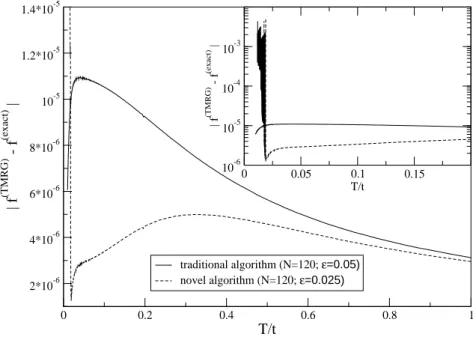
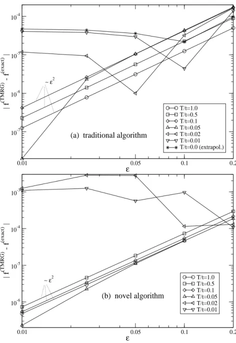
∼ O (), but astonishingly the error is in fact only of the order ∼ O ( 2 ) (see appendix A).
By inserting 2M times the identity operator a lattice path-integral representation of the partition function is derived:
Z = X
{s i k }
h α 1 | e −H o | α 2 i h α 2 | e −H e | α 3 i × · · ·
× h α 2M − 1 | e − H o | α 2M i h α 2M | e − H e | α 1 i (2.19) Here the state | α k i = | s 1 k i ⊗ | s 2 k i ⊗ · · · ⊗
s L k
with k ∈ [1, 2M ] and s i k being local basis states. Because H o , H e are sums of commuting terms we get
exp( − H e ) = Y
i=even
exp( − h i,i+1 ) , exp( − H o ) = Y
i=odd
exp( − h i,i+1 ) and the partition function becomes a matrix product
Z = X
{s i k }
τ 1,2 1,2 τ 1,2 3,4 · · · τ 1,2 L−1,L τ 2,3 2,3 τ 2,3 4,5 · · · τ 2,3 L,1
· · ·
τ 2M−1,2M 1,2 τ 2M−1,2M 3,4 · · · τ 2M L − 1,L −1,2M τ 2M,1 2,3 τ 2M,1 4,5 · · · τ 2M,1 L,1
(2.20)
1 This will be discussed in more detail in chapter 5 on the basis of the t-J model.
2 So M → ∞ means also → 0.
where
τ k,k+1 i,i+1 =
s i k s i+1 k
e − H e,o
s i k+1 s i+1 k+1
(2.21) is a local Boltzmann weight denoted in a graphical language by a shaded plaquette (see Fig. 2.2). The lower index represents the position in imaginary time whereas the upper index corresponds to the real space position. A possible choice for a transfer matrix is given by
T ˆ L = τ 1,2 τ 3,4 · · · τ L−1,L
τ 2,3 τ 4,5 · · · τ L,1
(2.22) with Z = Tr ˆ T L M . This transfer matrix evolves along the imaginary time direction (row-to- row transfer matrix). Because we want to perform the thermodynamic limit exactly and extend the transfer matrix numerically in imaginary time direction rather than in spatial direction, it is more convenient to rearrange the Boltzmann weights and to formulate a column-to-column transfer matrix (so-called quantum transfer matrix (QTM))
T M = (τ 1,2 τ 3,4 · · · τ 2M−1,2M ) (τ 2,3 τ 4,5 · · · τ 2M,1 ) = T 1 T 2 (2.23) evolving along the spatial direction, so that the partition function is given by
Z = Tr T M L/2 = X
µ
Λ L/2 µ (2.24)
with Λ µ being the eigenvalues of T M . This QTM for the classical model has checkerboard structure as shown in the left part of Fig. 2.2. It is also obvious from the graphical repre- sentation that the transfer matrix T M is not symmetric. If T 1 and T 2 are symmetric and semi-positive, it is possible to symmetrize T M analogously to the transfer matrix of the Ising chain (see Eq. (2.5)). However, this symmetrized form of the transfer matrix is use- less for numerical computations because it involves additional matrix products and also enhances the computer memory space needed to store these matrices. Additionally the conditions stated above are often not fulfilled for physically interesting models (e.g. spin models with a nonzero magnetic field) and it is therefore impossible in these cases to sym- metrize the transfer matrix. To determine eigenvalues and eigenvectors of non-symmetric matrices accurately is numerically much more complicated than for symmetric matrices which occur in ordinary DMRG calculations and is one of the main difficulties in TMRG algorithms. Details will be discussed in the next chapter.
The transfer matrix T M for the classical model derived by the traditional mapping is unnecessarily wide as the repeat length of the classical system is 2. This leads to several disadvantages discussed in detail later on. Here we will introduce a novel Trotter-Suzuki mapping [27] where the partition function is expressed by
Z = lim
M→∞ Tr n
[T 1 ()T 2 ()] M/2 o
with T 1,2 () = T R,L exp
− H + O ( 2 )
(2.25)
instead of Eq. (2.18). T R,L are the right- and left-shift operators, respectively. Detailed
calculations (see appendix A) show that the error of the mapping due to a finite is again
only of the order ∼ O ( 2 ) so that this mapping is a priori as well suited for numerical
calculations as the traditional one. The received classical lattice has alternating rows
666666777777
8 8 8 8 8
8 8 8 8 8
8 8 8 8 8
8 8 8 8 8
9 9 9 9
9 9 9 9
9 9 9 9
9 9 9 9 : : : :
: : : :
: : : :
: : : :
; ; ; ;
; ; ; ;
; ; ; ;
; ; ; ;
< < < < <
< < < < <
< < < < <
< < < < <
= = = =
= = = =
= = = =
= = = = > > > >
> > > >
> > > >
> > > >
? ? ? ?
? ? ? ?
? ? ? ?
? ? ? ? @A BCDE F FG GH HI I J JK K
LM NOPQ R RS ST TU U V VW W
XY Z[\] ^_`a bcde f fg gh hi i j jk k
lm nopq rstu vwxy z z{ {| |} } ~ ~
¡¡¡¡¡¡¡¡
¡¡¡¡¡¡¡¡
¡¡¡¡¡¡¡¡
¡¡¡¡¡¡¡¡
¢¢¢¢¢¢¢¢
¢¢¢¢¢¢¢¢
¢¢¢¢¢¢¢¢
¢¢¢¢¢¢¢¢
££££££££
££££££££
££££££££
££££££££
¤¤¤¤¤¤¤¤
¤¤¤¤¤¤¤¤
¤¤¤¤¤¤¤¤
¤¤¤¤¤¤¤¤
¥¦§¨ © ©ª
« «¬ ®
¯ ¯°
±²³´ µ µ¶
· ·¸ ¹ ¹º
» »¼
½ ½¾
¿ ¿À ÁÂÃÄ ÅÆÇÈ É ÉÊ
Ë ËÌ Í ÍÎ
Ï ÏÐ
Ñ ÑÒ
Ó ÓÔ ÕÖ×Ø ÙÚÛÜ Ý ÝÞ
ß ßà á áâ
ã ãä
å åæ
ç çè éêëì
í íî
ï ïð ñòóô
õ÷ö
ø÷ù ú÷û
ü
ü÷ý
ý
þ÷ÿ
!
"# $%
&' (())
**++ ,-
./
01
23 45
67
89
:; <=
>? @A
BC DD
EE
FG
quantum chain classical model
quantum chain classical model
QTM QTM
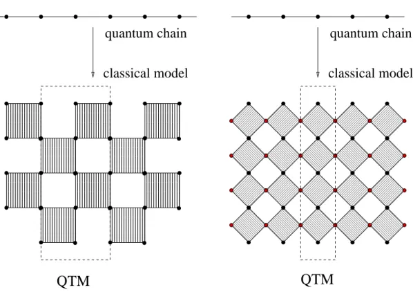
Figure 2.2: The left part shows the usual Trotter mapping of the 1D quantum chain to a 2D classical model with checkerboard structure where the vertical direction corresponds to imag- inary time. All lattice points of the classical model belong to the physical lattice at different imaginary time steps and the QTM is a two-column transfer matrix. The right part shows the alternative mapping as described in the text. The classical model has alternating rows and ad- ditional lattice points in a mathematical auxiliary space. The QTM in this formulation is only one column wide. In both figures the shaded plaquettes denote the same Boltzmann weight.
and additional lattice points in a mathematical auxiliary space but allows to formulate a QTM which is only one column wide as shown in Fig. 2.2. The derivation of this QTM is completely analogous to the one given before and the shaded plaquettes in Fig. 2.2 denote the same Boltzmann weight. The partition function with this new QTM, ˜ T M , is given by
Z = Tr ˜ T M L = X
µ
Λ ˜ L µ . (2.26)
Next, we will investigate the spectra of the two QTMs at infinite temperature where a local Boltzmann weight reduces to (see Fig. 2.3)
τ (s 1 , s 2 | s 0 1 , s 0 2 ) = δ s 1 ,s 0 1 δ s 2 ,s 0
2 . (2.27)
As shown in Fig. 2.4 the relations
T M 2 = n 2 T M , T ˜ M = n T ˜ M
Tr T M = n 2 , Tr ˜ T M = n (2.28)
s 1 ’ s 2 ’
s 1 s 2 s 1 s 2
s 1 ’ s 2 ’
s 1 s 1 ’ δ ,
δ s s ’ 2 , 2
0 0
T
Figure 2.3: The Boltzmann weight (plaquette interaction) in the limit T → ∞ .
= n 2
eigenstates
:
eigenstates
= n 2
= n
T M 2 T M
= n
T M 2 T M
= n
: = n
Figure 2.4: The relations for T M 2 (upper part) and Tr T M (lower part) are depicted graphically for the traditional QTM (left part) and the novel QTM (right part).
for the old QTM (left relations) and new QTM (right relations) are easy to prove. Here
n denotes the number of possible values of the classical variable s i k . The upper relations
lead to Λ = n 2 ∨ Λ = 0 (Λ = n ∨ Λ = 0) for the eigenvalues of the old (novel) QTM
at infinite temperature, whereas the lower relations show additionally that the largest
eigenvalue is given by Λ 0 = n 2 (Λ 0 = n) and all other eigenvalues are zero in both
cases. The gap between the leading and next-leading eigenvalues of the QTM becomes
smaller with decreasing temperature. However, we expect that the gap vanishes only at
zero temperature because a vanishing gap indicates a diverging correlation length (see Eq. (2.16) or (2.34)), i.e. a critical point or a certain kind of long range order which are expected to be present in a 1D quantum system only at zero temperature. This has been proved by Mermin and Wagner [5] for ferro- or antiferromagnetic order in 1D Heisenberg models. Therefore the free energy at non-zero temperature with fixed Trotter number M is determined in the thermodynamic limit solely by the largest eigenvalue of the QTM
f ∞ ,M = − T lim
L→∞
1
L ln Z = − T lim
L→∞
1 L ln
( X
µ
Λ L µ )
= − T lim
L→∞
1 L ln
Λ L 0
1 +
Λ 1
Λ 0 L
| {z }
L→∞ −→ 0
+ Λ 2
Λ 0 L
| {z }
L→∞ −→ 0
+ · · ·
L→∞ −→ − T ln Λ 0 . (2.29)
Note that this is the free energy of a system with dimension ∞× M , i.e. there are still finite size corrections of the order ∼ O ( 2 ) present. The additional limit → 0 in Eq. (2.29) yields the desired result for the quantum chain because the limits L → ∞ and → 0 are interchangeable as shown by Suzuki [15]. The formula (2.29) is valid for the novel QTM whereas T has to be replaced by T /2 for the checkerboard QTM. 3 In principle, all other thermodynamic quantities can be derived from the free energy by numerical derivatives. However, for some quantities (e.g. magnetization or particle number) it is easier to calculate them directly in the following way. Let us consider the thermal average of a local operator O 1,2 acting at sites 1 and 2, which commutes with the local Hamiltonian h i,i+1 :
h O 1,2 i = lim
L→∞
1
Z Tr O 1,2 e −βH
= lim
L→∞
1
Z Tr T M (O 1,2 )T M L−1
→
Ψ L 0
T M (O 1,2 ) Ψ R 0 Λ 0
(2.30) Here
Ψ L 0 and
Ψ R 0
are the right and left eigenvectors, respectively, belonging to the largest eigenvalue Λ 0 of T M . The modified transfer matrix is given by
T M (O 1,2 ) = (τ 1,2 (O 1,2 )τ 3,4 · · · τ 2M −1,2M ) (τ 2,3 τ 4,5 · · · τ 2M,1 ) (2.31) with
τ 1,2 (O 1,2 ) = s 1 1 s 2 1
O 1,2 e − h 1,2 s 1 2 s 2 2
. (2.32)
3 All following relations are valid for the novel QTM. For the checkerboard QTM L has to be replaced
by L/2 leading sometimes to an additional factor 1/2 but leaving the formulas otherwise unchanged.
In a similar way it is also possible to receive a formula for a two-point correlation function h O 1 O r i =
Ψ L 0
T M (O 1 )T M r−1 T M (O r ) Ψ R 0
Λ r+1 0 (2.33)
= h O 1 i h O r i + X
n6=0 n
Ψ L 0
T M (O 1 )
Ψ R n Ψ L n
T M (O r ) Ψ R 0 Λ 0 Λ n
Λ n Λ 0
r
= h O 1 i h O r i + X
n n 6 =0
Ψ L 0
T M (O 1 )
Ψ R n Ψ L n
T M (O r ) Ψ R 0 Λ 0 Λ n
| {z }
M n
e −r/ξ n e ik n r
where the correlation lengths ξ n and wavevectors k n are given by ξ n − 1 = ln
Λ 0 Λ n
, k n = arg Λ n
Λ 0
. (2.34)
Note that Eq. (2.33) gives an expansion of the correlation function (CF) of the form h O 1 O r i − h O 1 i h O r i = P
n M n e −r/ξ n e ik n r with matrixelements M n . The long distance be- haviour is dominated by the correlation length (CL) ξ α belonging to the largest eigenvalue Λ α (α 6 = 0) which satisfies the condition M α 6 = 0. 4 Note also that several CLs ξ with the same wavevector k can appear in the asymptotic expansion displayed in Eq. (2.33). In the structure factor each term yields a (measurable) Lorentz function
S n (k) = M n 2π
Z ∞
−∞
dr e −| r | /ξ n e i(k n − k)r = M n πξ n
1
(k − k n ) 2 + 1/ξ n 2 (2.35) with center at k n , height ∼ M n ξ n /π and width ∼ 2/ξ n . The sharpest peak corresponds to the leading instability towards the onset of long range order and hence, a crossover in the leading CL indicates a change of the nature of the long range order. Using Eq. (2.35), it is possible to determine the CL, wavevector and matrixelement by neutron scattering experiments (see e.g. [28]) so that these quantities are not only of theoretical interest.
In addition, it is also possible to calculate imaginary time correlations G(r, τ ) directly within the TMRG algorithm [26]. The fatal point is that the analytical continuation of imaginary time results with numerical errors to real times is an ill-posed problem leading to unreliable results. We will return to this point in chapter 7. What is calculated without fundamental problems are static CFs 5 defined by
G(r, z = 0) = Z β
0
dτ G(r, τ ) . (2.36)
This CF can be expressed by the largest eigenvalue and the corresponding left and right eigenvectors h Ψ L 0 | , | Ψ R 0 i of the QTM:
G(r, z = 0) =
M Λ r+1 0 h Ψ L 0 | T ˜ M T M r−1 T ˜ M | Ψ R 0 i with T ˜ M =
M
X
k=0
T M (A ·k ) (2.37)
4 We are interested in a few leading correlation lengths, i.e. in the asymptotic behaviour at large distances.
5 Here static means ω = 0, but it is also possible to calculate equal time correlation functions (t = 0)in
a similar way .
for distances r ≥ 1, where T M (A ·k ) denotes the usual transfer matrix T M with the con- sidered operator A added at imaginary time position τ = · k. The static autocorrelation has to be treated separately
G(r = 0, z = 0) =
Λ 0 h Ψ L 0 | T ˆ M | Ψ R 0 i with T ˆ M =
M
X
k=0
T M (A 0 , A · k ) . (2.38)
After deriving the formulas for the CL and static CF, we can now discuss the disadvan- tages of the checkerboard decomposition in comparison to the novel mapping: (1) The wavevector k of a CF (see Eq. (2.34)) is not uniquely determined in the checkerboard decomposition , i.e. this QTM cannot distinguish between k and k + π; (2) the calculation of CFs (see Eqs. (2.37),(2.38)) is much more complicated, because even and odd as well as distance 1 have to be treated separately; (3) the cost of computer memory is unnecessarily large due to the repeat length of 2. This will be explained in detail in the next section.
Unfortunately, there is also one disadvantage of the novel QTM one should mention. The left and right eigenstates of this non-symmetric matrix have to be calculated separately whereas this is not necessary for the checkerboard QTM due to additional symmetries.
We will also discuss this point in detail in the next section.
2.2 The algorithm
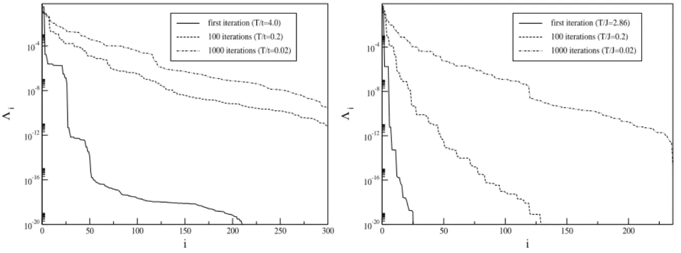
In this section we will describe how the length of the transfer matrix in imaginary time direction can be extended iteratively using the DMRG scheme. With increasing Trotter number M the dimension of the transfer matrix grows exponentially and the task is to truncate this matrix in an optimal way so that even large Trotter numbers up to M ∼ 2000 can be handled on a computer. For a Hamiltonian system the thermodynamic density matrix is usually defined by
ρ th = e −βH . (2.39)
In ordinary zero-temperature DMRG a chain of length L (so called superblock) is divided into two equal parts which are called system block S and environment block E. A reduced density matrix ρ S is defined by performing a partial trace with respect to the environment:
ρ S = Tr E ρ th . It has been shown that the eigenvectors of this matrix corresponding to the largest eigenvalues are in some sense the optimal set of system block states to represent the ground state in a reduced basis. 6 The transfer matrix is treated rather similarly to the quantum chain. We always take an even number of local Boltzmann weights, cut the transfer matrix T M (superblock) in the middle and call one part system and the other environment block. A generalized density matrix in Trotter space is then defined by
ρ = T M L (2.40)
6 For details see [11] and Noack, White in [26].
which reduces in the thermodynamic limit to ρ =
Ψ R 0 Ψ L 0
up to a normalization con- stant due to the gapped spectrum of T M . A reduced density matrix is again defined by performing a partial trace with respect to the environment
ρ S = Tr E
Ψ R 0 Ψ L 0
. (2.41)
Note however that this matrix is not symmetric and it is therefore not clear whether the eigenvalues are semi-positive. Indeed a proof has been given only in a few special cases [26]. However, numerically we find that this is more or less true in all considered systems. 7 We want to emphasize that the “reduced density matrix” is only used to select the reduced basis and the results decide whether this truncation scheme is appropriate or not. Whether it is really a density matrix with a probability interpretation of its eigenvalues is a purely academic question, which is not important for the numerical ap- proach. Taking this “problem” seriously, Bursill et al. [16] and others have suggested a symmetrized version
ρ 1 symm =
Ψ R 0 Ψ R 0
, ρ 2 symm =
Ψ L 0 Ψ L 0
or even ρ 3 symm =
Ψ R 0 Ψ R 0 +
Ψ L 0 Ψ L 0 , (2.42) but these are no longer projection operators onto the ground state 8 leading to a bad representation of the ground state in the truncated Hilbert space and to an algorithm that breaks down rapidly after a relatively small number of RG steps. Therefore we will always use in our calculations the non-symmetric reduced density matrix defined in Eq. (2.41).
In practical computations the small parameter in the Trotter-Suzuki mapping (see Eqs. (2.18) and (2.25)) is fixed where = 0.025 to 0.05 has turned out to be a suit- able choice. The temperature is then given by T ∼ 1/M and is decreased by an iterative algorithm where M → M + 1. Here and in the following M denotes the number of lo- cal Boltzmann weights (plaquettes) in the system block. The complete QTM therefore consists of 2M plaquettes. In the following we discuss the algorithms for the checker- board QTM (see a) below) as well as for the novel QTM (see b) below). Whereas the algorithm for the checkerboard QTM closely follows the one outlined by Wang, Xiang and Shibata [17, 18], we have formulated a modified one for the novel QTM, which takes advantage of the different transfer-matrix structure and allows us to reduce the required computer memory drastically. Note that it is also possible to formulate the algorithm for the novel QTM completely analogous to the traditional one, but in this case the same amount of memory is needed. In all steps and both algorithms the cases M even and odd have to be treated separately. In the following the column-to-column transfer matrices (QTMs) are shown in a 90 ◦ -rotated view.
1) We start by constructing an initial system block Γ containing M plaquettes so that a) S M−1 ≤ N < S M or b) S M ≤ N < S M+1 where S denotes the dimension of the local Hilbert space and N is the number of states which we want to keep within the
7 Sometimes eigenvalue pairs with small imaginary parts occur as discussed in chapter 3.
8 That means, e.g.
Ψ L 0
ρ 3 symm = a Ψ R 0
+ b Ψ L 0
6 = Ψ L 0
with some normalization constants a, b 6 = 0.
renormalization. The plaquettes are connected by a summation over the adjacent corner spins (structure of a tensor product).
s 1 s 2
a) σ τ b)
n’ s n s
σ τ
n s
n’ s
Each so called block-spin variable n s , n 0 s contains in the initial step a) ˜ N = S M − 1 or b) ˜ N = S M states. The a) S 4 · N ˜ 2 -dimensional array Γ(s 1 , n s , s 2 , σ, n 0 s , τ ) or b) S 2 · N ˜ 2 -dimensional array Γ(σ, n s , τ, n 0 s ) is stored.
2) a) The superblock T 2M is built by connecting the system block and the environ- ment block by a τ-summation where the environment block is constructed anal- ogously to the system block or is just given by a 180 ◦ -rotation of the system block if the local interaction is reflection symmetric, i.e. h i,i+1 = h i+1,i . This is the case for all models considered here.
b) A plaquette is added to the system block to form the enlarged system block Γ(σ, n ˜ s , s 2 , τ, s 0 2 , n 0 s ) which is a S 4 · N ˜ 2 -dimensional array. The same is done for the environment block. If h i,i+1 is real, the environment block can be constructed by a 180 ◦ -rotation and a following inversion of the system block.
A reflection symmetry is not needed! 9 The enlarged blocks are connected to form the superblock T 2M+2 .
s 1 s 2
s’ 2 s’ 1
s 2 s 1
s’ 2 s’ 1
a) σ σ b)
n’ s
n s n e
n’ e
σ σ
n s
n’ s
n e
n’ e
In both cases the superblock is closed periodically by a summation over all σ-states.
3) The largest eigenvalue Λ 0 and the corresponding left and right eigenstates Ψ L 0
= Ψ L (s 1 , n s , s 2 , n e ), Ψ R 0
= Ψ R (s 0 1 , n 0 s , s 0 2 , n 0 e ) of the superblock are calculated. The eigenvectors are normalized by
Ψ L 0 | Ψ R 0
= 1.
If correlation lengths are needed, next-leading eigenvalues have to be calculated additionally.
9 This might be interesting for models with next-nearest neighbour interactions where 2 sites are
combined to a supersite in order to receive a local Hamiltonian ˜ h i,i+1 containing only nearest neighbour
interactions and being translationally invariant. However, ˜ h i,i+1 6 = ˜ h i+1,i making it necessary to store and
renormalize the environment block explicitly within the checkerboard formalism. The new QTM allows
it even in this case to construct the environment from the system block and therefore saves computer
memory and computing time.
4) At the temperature a) T = 1/M or b) T = 1/(2M + 2) the free energy, correlation lengths and other thermodynamic quantities are evaluated.
5) The density matrix is given by a) ρ = T 2M L/2 /Tr T 2M L/2 or b) ρ = T 2M L +2 /Tr T 2M+2 L and reduces in both cases in the thermodynamic limit to ρ =
Ψ R 0 Ψ L 0
due to the gapped spectrum of the QTMs. A reduced density matrix is now calculated by performing a partial trace with respect to the environment
ρ s (n 0 s , s 0 2 | n s , s 2 ) = X
s 1 ,n e
Ψ R 0 Ψ L 0
= X
s 1 ,n e
Ψ R (s 1 , n 0 s , s 0 2 , n e )Ψ L (s 1 , n s , s 2 , n e )
and the complete spectrum of this non-symmetric matrix is determined. If the Hamiltonian has no spatial reflection symmetry, a second reduced density matrix ρ e has to be calculated in case a) by performing a partial trace with respect to the system. The left (right) eigenstates of ρ s corresponding to the N largest eigenvalues are used to construct a N × (S · N ˜ )-matrix V L (˜ n s | n s , s 2 ) (V R (˜ n 0 s | n 0 s , s 0 2 )) where ˜ n s (˜ n 0 s ) is a new, renormalized block-spin variable. The eigenstates are normalized satisfying the orthonormality relation (V L ) T · V R = 1.
6) a) The system block is enlarged by adding a plaquette to form the enlarged sys- tem block ˜ Γ(s 1 , n s , s 2 , τ, σ, n 0 s , s 0 2 , ˜ s 0 2 ) which is a S 6 · N ˜ 2 -dimensional array. The matrices V L and V R are used to truncate the Hilbert space and to receive new block-spin variables ˜ n s , n ˜ 0 s taking only N possible values. If no spatial reflection symmetry is present, the same is done for the environment block.
b) The system block is renormalized by applying V L and V R . New block-spin variables ˜ n s and ˜ n 0 s are received.
s 1 s 2
s’ 2 s 2
s 1 s 2
s 2
s’ 2
s 2
s’ 2