arXiv:1210.5748v1 [quant-ph] 21 Oct 2012
Quirin Hummel1, Juan Diego Urbina and Klaus Richter
Institut f¨ur Theoretische Physik, Universit¨at Regensburg, D-93040 Regensburg, Germany
E-mail: 1quirin.hummel@physik.uni-regensburg.de
Abstract. We present a novel analytical approach for the calculation of the mean density of states in many-body systems made of confined indistinguishable and non- interacting particles. Our method makes explicit the intrinsic geometry inherent in the symmetrization postulate and, in the spirit of the usual Weyl expansion for the smooth part of the density of states in single-particle confined systems, our results take the form of a sum overclustersof particles moving freely around manifolds in configuration space invariant under elements of the group of permutations. Being asymptotic, our approximation gives increasingly better results for large excitation energies and we formally confirm that it coincides with the celebrated Bethe estimate in the appropriate region. Moreover, our construction gives the correct high energy asymptotics expected from general considerations, and shows that the emergence of the fermionic ground state is actually a consequence of an extremely delicate large cancellation effect.
Remarkably, our expansion in cluster zones is naturally incorporated for systems of interacting particles, opening the road to address the fundamental problem about the interplay between confinement and interactions in many-body systems of identical particles.
PACS numbers: 74.20.Fg, 75.10.Jm, 71.10.Li, 73.21.La
1. Introduction
Understanding the general physical properties of interacting systems is one of the ultimate goals of classical and quantum mechanics, and probably the most difficult.
An impressive toolbox including techniques such as the renormalization group [1, 2], perturbation expansions in Feynman diagrams [3,4] and Density Functional Theory [5,6]
has been developed during the past decades with the sole objective of constructing the energy spectrum of quantum systems where external potentials, inter-particle interactions and quantum statistics must be simultaneously considered.
In a non-relativistic first-quantization scenario (which is an effective low-energy approximation to the fundamental field-theoretical relativistic description) both the Hilbert space and the Hamiltonian are fairly well understood and the problem of constructing the energy spectrum is reduced to the, still formidable, problem of calculating the many-body density of states
̺±(E, N) =−1 πℑh
tr(N)± G(Eˆ +iǫ)i
. (1)
Here N is the total number of particles, (±) refers to the symmetry with respect to particle exchange of the subspace where the trace operation is performed (fully symmetric wavefunction for bosons and fully antisymmetric one for fermions), and ˆG is the Green function of the many-body system, defined in terms of the full interacting Hamiltonian
Hˆ = ˆH0+gUˆ (2)
as
G(z) =ˆ
z−Hˆ−1
, (3)
where ˆH0 describes a set of non-interacting particles, ˆU is the (two-body) interaction potential and g the coupling strength.
In this paper we are interested in the situation where the quantum system is made up of well defined microscopic degrees of freedom either bosonic or fermionic, subject to a hard wall confinement in D dimensions such that the system is bounded for all energies. In this case, the density of states has the generic form
̺±(E, N) = X
n
δ(E−En(N)), (4)
where n = 1,2. . . labels the ordered eigenvalues E1(N), E2(N), . . . of ˆH for fixed total number of particlesN. Although the precise knowledge of the density of states provides all the information about the spectrum of the system, general considerations show that
̺±(E, N) can be unambiguously decomposed into a smooth and an oscillatory part,
̺±(E, N) = ¯̺±(E, N) +̺osc± (E, N), (5) where the scaling of the smooth part is given asymptotically by the Weyl formula [7–9]
¯
̺±(E, N)∼1/~DN. (6)
the total energy and the classical many-body dynamics is chaotic, for the oscillatory part we can formally apply the Gutzwiller trace formula [10, 11] to get
̺osc± (E, N)∼1/~ (7)
in the semiclassical limit ~ → 0 ‡. From the scaling with ~ in the semiclassical limit it is expected that oscillatory contributions to the many-body density of states in the strongly interacting regime where the quantum mechanical description of the system lies beyond the single-particle picture, are extremely small compared to the mean density
¯
̺±(E, N). Understandably, continuous effort has been dedicated to develop methods to construct this function either numerically or analytically [4, 11, 13–15].
To date, the only general way to obtain the precise ¯̺±(E, N) is by explicit (typically numerical) diagonalization techniques of the many-body problem followed by a convolution with a smoothing function Wǫ(E) of width ǫ,
¯
̺±(E, N) = ˆ ∞
−∞
̺±(E, N)Wǫ(E)dE . (8)
However, due to the fast (exponential) growth of the basis required to achieve good convergence of the numerical results, such numerical approaches can deal with only moderate numbers of particles (see, e.g., [16] for state of the art calculations).
Given the complexity of the problem, alternative methods are mandatory. Self- consistent mean-field methods, firmly grounded in the Kohn-Sham theorem [5, 6], provide the most efficient way to construct a set of single-particle wavefunctions such that the ground state energy of the interacting system can be systematically approximated by artificial single-particle energies supplemented with the appropriate symmetry of the many-body wavefunction.
Despite the extremely successful application of self-consistent methods, ranging from nuclear physics to molecular systems, reaching chemical problems [5, 6, 17], the calculation of the many-body density of states within mean-field approaches faces a conceptually deep and basically unsolved problem. It is related with its very definition, and stems from the fact that the calculation of different types of observables actually requires a different definition for the mean field. Examples of this ambiguity are the calculation of ground-state vs excited-state energies and the construction of static vs dynamical properties of the system (for the calculation of transition amplitudes, for example, the mean field is necessarily time-dependent and depends on the initial and final states as well) [4].
To be more precise, extending self-consistent approaches like the Density Functional Theory or Hartree-Fock method to excited states above the ground state requires a specific knowledge of which single-particle orbitals are optimized through the self- consistent equations, and therefore each excited many-body state requires a separated
‡ We do not discuss questions [12] concerning the derivation of (7) forDN ≥3 here.
calculation leading to a different mean-field. Similar problems appear in formulations of the many-body problem based on a functional representation of the propagator where the mean-field is defined by means of a saddle-point equation: roughly speaking, the single-particle artificial potential used to mimic the effects of interparticle interactions becomes dependent on the excitation energy itself [4].
Working with a mean-field which is simply a function of the position, independent on both excitation energy and/or time is then a strong assumption that lies behind much of the efforts to understand many-body systems in terms of a single-particle picture, an assumption which is in fact turned into essential in most cases where even a mild dependence of the mean field on the excitation energy would make the calculations impossible.
Luckily, many important physical effects accessible to experimental observation take place near or at the ground state energy, and it is expected that in this situation the mean field, providing the independent particle picture for the ground state within any of the self-consistent methods, can be used to calculate physical properties of excited states with decreasing accuracy as we move to higher and higher excitation energies.
This physical consideration, together with the more pragmatic reasons explained above, has shown to be remarkably useful. In fact, the idea of an unique mean field allows us to use all the standard machinery of single-particle physics as input for the statistical mechanics results for independent particles and to finally produce experimentally accessible predictions beyond the strictly non-interacting case. A good mean field is then an excellent starting point.
A paradigm of the success of this approach is the study of low energy excitations of bounded fermionic systems with many particles like nuclei, metallic clusters and quantum dots [5, 6, 17]. Here, a self-consistent calculation of variational type is set up to fix once and for all a single-particle potential responsible to replace the interparticle interaction. The result of the numerical calculation is used then to fit the parameters of a large family of functional forms (e.g. Woods-Saxon for nuclei [18–20]) to finally produce an analytical form. Once this is achieved, standard methods of statistical physics are applied.
A result of these studies which is of importance for the present work is that, for a large enough number of electrons interacting through Coulomb forces in a billiard- shaped quantum dot, the mean field (in the sense of Hartree-Fock) closely follows the billiard potential. This allows us to assume a billiard model for the interacting system in mean field approximation knowing that it already captures part of the physics beyond the non-interacting case through a softening of the boundaries.
The program outlined above has reached a high sophistication, in particular when the single-particle physics is treated analytically by means of semiclassical methods, well suited to study the effective single-particle problem around the Fermi energy for the regime of large numbers of particles. The idea here is to construct the single-particle spectrum in terms of periodic orbits of the classical system considered as a single-particle moving within the mean field potential. The amount of work on the subject is huge and
like the existence of shell effects visible in the many-body density of states and due to continuous families of classical periodic orbits.
Another possibility offered by the mean field approach comes from one of the main lessons we have learnt from single-particle systems, namely that contrary to ̺±(E, N) which would be sensitive to every single detail of the microscopicmean fieldHamiltonian, the smooth part of the density of states ¯̺±(E, N) predominantly depends on few classical quantities related to the measure of the classical phase space manifolds at given energy. Therefore, instead of going through numerically expensive calculations in order to construct the single-particle energies in mean field approximation just to average out again the density of states and get its smooth part as indicated by (8), one can try to construct and understand the classical phase-space structures behind . This approach can be carried on in two different and complementary ways.
The first option is to push the mean field picture and calculate the smooth part of the single-particle density of states using the Thomas-Fermi approximation and its variants [11], and use it together with well established statistical techniques to construct
¯
̺±(E, N). This is the line of thought that lies behind the original attempt of Bethe [13]
to calculate the smooth part of the level density for nuclei and, more recently, a similar concept is followed in the seminal works of Weidenm¨uller [21] in order to formally construct the exact level density ̺±(E, N) for non-interacting particles. It is important to mention that this approach is based on the classical single-particle phase space, and the construction of the many-body density of states is purely formal and has no direct interpretation in terms of the classical many-bodyphase space.
The second possibility, namely, to calculate the smooth part of the many-body density of states in mean field approximation by relating it directly to the structure of the many-body classical phase space has not been systematically addressed before. In our opinion, such approach has the potential advantage of avoiding the a prioriconflict with the inclusion of residual interactions inherent to any approach that is based on the single-particle phase space.
As we will show, these two approaches give quite different points of view for the calculation of ¯̺±(E, N), and their equivalence for the strict mean field limit is by no means trivial. However, once this equivalence is established, our methods based on the many-body phase space will allow to address the fundamental question concerning how the relevant geometrical structures are translated into the problem in the presence of residual interactions. This is the program we propose here.
Once the single-particle picture is adopted the study of reference is the so-called Bethe estimate, providing an asymptotic result for the density of states in many-fermion systems in mean field approximation, valid for energies far enough (in units of the single-particle mean level spacing) from the ground state EGS and large numbers of particles [13],
¯
̺±(E, N)≃ e
q2π2
3 ̺¯sp(EF)(E−EGS)
√48(E−EGS) . (9)
The essential aspect of Bethe’s result in the context of interest here is that it is an asymptotic approximation for the smooth part of the density of states, and can be interpreted as the fermionic analogue of the Weyl expansion for billiard systems.
However, and despite its enormous importance, (9) (and the thermodynamic formalism used in its derivation) is of limited use for us, as it does not provide any clue on how classical phase space manifolds work together to produce both its characteristic functional form and the scale EGS.
In the physical scenario of interest here (the application of Bethe’s method in confined electronic systems) the most relevant problems besides the all long issue of residual interactions are, i) the inclusion of finite N effects, ii) the consistent treatment of the ground state energy and the density of states around it, and iii) the emergence of the standard Weyl expansion ¯̺±(E, N) ∼EDN/2−1 for high enough energies. These questions have been addressed already, and the amount of literature in the subject is extensive, so we will only briefly review the state of the art.
Finite size effects on the asymptotic density of states in systems of fermions can be systematically calculated in mean field approximation by extending Bethe’s result, which is the leading order in an expansion valid for large excitation energies and large numbers of particles obtained by a saddle point approximation of the exact grand-canonical partition function [4, 13–15]. Because the problem of counting many-body eigenstates for non-interacting identical particles has a natural combinatorial formulation, this approach has produced an unexpected and fruitful interaction with number theory.
In this spirit, corrections to the Bethe estimate arising from finite number of particles, oscillatory corrections to the single-particle density of states, and shell effects affecting the ground state energy have been considered [22].
The status of the ground state energy within the asymptotic approach is somehow delicate, as strictly speaking, the many-body density of states must vanish identically for energies bellow EGS. As obvious as this observation may be, it turns out that it is extremely difficult to construct a theory providing the large energy asymptotics for
¯
̺±(E, N) while keeping this condition exact. This problem may be considered at first glance a merely academic, since after all no physical process takes place for energies bellow the ground state, and the later has a very precise definition in terms of the single-particle density of states. We must however keep in mind that the final goal of any approach is to deal with the fully interacting system and/or to provide insight and better methods to define and calculate the mean field and the effect of the residual interactions. Beyond the mean field picture, we eventually need a systematic method to identify and construct the ground state energy independent of the counting prescription valid in the non-interacting case. To the best of our knowledge, a systematic study of how do approximations for ¯̺±(E, N) behave for E < EGS is missing.
Finally, very general and robust considerations demand that asymptotically (when the energy goes to infinity), essential quantum mechanical effects such as the non-zero ground state energy gradually disappear and a purely classical description emerges. In this limit, one should recover the standard Weyl expansion for the density of states
phase space to a fraction of 1/N! due to the identity of the particles but not to their particular statistics [23]. Using asymptotic methods to understand this transition leads to some interesting results connected with the number-theoretical formulation of the problem [22].
Together with the goal of providing a geometrical approach to ¯̺±(E, N), the last paragraphs indicate the main motivations of the present work. We attempt to provide a method to construct the Weyl approximation to the smooth part of the density of states which relies only on kinematic and geometrical aspects within the mean field approximation. As expected, our results are connected with several others (in particular with Bethe’s) and an important aspect of our work is to make these connections explicit.
However, the method itself and the physical idea behind it, namely that the Weyl expansion can be systematically constructed out of free propagation near symmetry manifolds are our novel contributions to the subject.
The paper is organised as follows. In section 2 we introduce the basic notation and briefly review the construction of the Weyl expansion for systems of non-interacting identical but distinguishable particles. In sections 3 and 4 the symmetrization postulate is used to give the formal expression for the full density of states for indistinguishable particles, and we show how this formal object can be understood in terms of the geometry of a higher dimensional phase space when the fundamental domain associated with the group of permutations SN is considered. The role of classical manifolds invariant under different elements of the symmetric group is clearly seen using the example of two fermions on a line in section 5. The very non-trivial generalization of this construction for arbitrary type of particles (bosons or fermions), arbitrary dimension D of the single-particle configuration space Ω and arbitrary number of particles N is fully carried out in sections 6 and 7 and culminate with a full identification of the classical manifolds and their measures responsible for the functional form of ¯̺±(E, N) and the emergence of EGS. We analyse our results in sections 8 and 9, where the equivalence of our results with the Weidenm¨uller convolution formula and with Bethe’s estimate are rigorously proved. We conclude and discuss the extension of our results for the interacting case in section 10.
2. Non-interacting Distinguishable Particles
First consider a billiard system of N non-interacting, identical, but distinguishable particles in D dimensions, specified by their coordinates
qi ∈RD, i= 1, . . . , N (10)
with spatial components
qi(d) ∈R, d= 1, . . . , D . (11)
This corresponds to an effective N ·D-dimensional billiard system of a single particle described by
q= (q1, . . . ,qN)∈RN D. (12) In this case the only effect of particle exchange symmetry is thereby the existence of discrete spatial symmetries in the effective higher dimensional single-particle system.
But due to distinguishability, there is no restriction to any subset of wavefunctions with specific symmetry under exchange transformation.
In general, the density of states (DOS) of a bound, time independent system can be expressed as the inverse Laplace transform of the trace of the propagator Uˆ(t) = exp(−i/~Ht):ˆ
̺(E) =L−1
β
ˆ
dN Dq K(q,q;t=−i~β)
(E), (13)
where the trace is performed in coordinate space withK(q′,q;t) =hq′|Uˆ(t)|qiand the inverse Laplace transform has to be applied with respect to the variable β.
In semiclassical approximation (corresponding to the formal limit ~→0) there are two contributions to the DOS
̺scl(E) = ̺osc(E) + ¯̺(E), (14) one oscillating (̺osc) and one smooth (¯̺) in the energy E. The oscillatory part arises from various stationary phase approximations in (13) starting from a path integral representation of the propagator. The process leads to a description by periodic orbits of the underlying classical system. The oscillatory part of the DOS is then in semiclassical approximation expressed by the Gutzwiller trace formula in the chaotic case [10,24] and the Berry-Tabor trace formula in the integrable case [25] respectively.
The smooth part of the DOS is related to short path contributions that are not caught by periodic orbits in the analysis of the trace of the propagator. Reflecting the short time behaviour of the propagator, these are related to the assumption of local free quantum propagation and additional boundary corrections [26]. The Weyl expansion for the N ·D-dimensional billiard reads [26]
¯
̺(E) = m 2π~2
N D2 VN D
Γ N D2 EN D2 −1θ(E)
± 1 4
m 2π~2
N D−12 SN D−1
Γ N D−12 EN D−12 −1θ(E) +· · ·.
(15)
The first term in (15) will be referred to as the volume Weyl term and equals the Thomas-Fermi approximation ¯̺TF(E) [11] proportional to theN·D-dimensional volume VN D. The second term originates from wave reflection near billiard boundaries under the assumption of local flatness of the surface. This involves free quantum propagation to mirror points yielding a fast converging integral over the coordinate perpendicular to
coordinates yielding the surface SN D−1 (not to be confused with the symmetric group SN) of the billiard instead of its volume. Higher corrections in the expansion correspond to propagation between multiply reflected image points accounting for curvature, edges or corners of the boundary.
3. Non-interacting Undistinguishable Particles
In the case of N identical particles that are undistinguishable, the state of the system obeys a specific symmetry with respect to particle exchange. The state is either symmetric or antisymmetric under the exchange of any two particles, depending on whether they are bosons or fermions.
Pˆ|ψ±i= (±1)P |ψ±i, (−1)P := sgn(P) (16) for any permutationP ∈SN, where ˆP is the corresponding permutation operator acting on many-body states, and plus and minus refer to bosons respectively fermions. In order to obtain the physical spectrum of such a system one has to restrict to those eigenenergies that correspond to the subspace of Hilbert space with appropriate symmetry. Let ˆ
1± = ˆ1†± be the projector onto the subspace of correct symmetry. Restricting the trace in (13) to this subspace is equivalent to replacing the propagator by its symmetry projected analogue
Uˆ±(t) := ˆ1±Uˆ(t)ˆ1± = ˆ1±Uˆ(t), (17) K±(q′,q;t) := 1
N! X
P∈SN
(±1)P K(Pq′,q;t). (18) In (17), the commutation of the time evolution operator and the symmetry projector due to [ ˆP ,H] = 0 and idempotence of ˆˆ 1± have been used. This leads to the symmetry projected DOS
̺±(E) =L−1
β
"
1 N!
X
P∈SN
(±1)P ˆ
dN Dq K(Pq,q;t=−i~β)
#
(E). (19) Thus symmetry causes the need of taking wave propagation over finite distance into account, asPq6=qin general. For the oscillating part in̺±(E) it is possible to construct a fundamental domain in phase space where it is again sufficient to find periodic orbits and additionally the group characters (±1)P of the group elementsP connected to each trajectory (q,p)7→(Pq, Pp) in the unfolded full domain [27]. However this procedure has no direct application to the smooth part of the DOS in the general case of arbitrary particle number and spatial dimension.
This is true even in a bosonic system in D > 1 despite the possibility of mapping it to the higher dimensional system of a single particle without symmetry moving in the fundamental domain in coordinate space with topological identification
of symmetry related points. That is because of the non-trivial structure of such a wrapped fundamental domain especially in the vicinity of symmetry planes defined by Pq = q for some P ∈ SN. In order to illustrate this, compare to a two dimensional single-particle system with discrete rotational symmetry
[ ˆH,Rˆφ] = 0, Rˆφ= exp
−i
~Lˆzφ , φ= 2π
n , n∈N.
(20)
The restriction to the subspace of states symmetric under the elementary rotation Rˆφ|ψsymi=|ψsymi is equivalent to the restriction to the wrapped fundamental domain with usual wave dynamics. The wrapped fundamental domain in this example is the restriction of the billiard to a sector of central angleφwith identification of points along its two bordering half-lines. As it is equal to a cone, this produces non-trivial wave propagation at the origin which gives rise to additional corrections in the level density
¯
̺sym(E) of symmetric states [28]. Analogue to that, mapping a bosonic system to its wrapped fundamental domain implies non-trivial wave propagation in the vicinity of the symmetry planes. This shows that it is reasonable to stay in the full domain for the calculation of the smooth part ¯̺±(E), and this is the approach we will follow here.
Previous to the treatment of the general case it is instructive to analyse the simple example of many identical fermions on a line which can be mapped to a fundamental domain where the additional correction due to symmetry can easily be obtained by usual methods.
4. Equivalence of Many-Body and High Dimensional Single-Particle Pictures
This section will mainly focus on systems of many fermions moving on a line of length L. These systems have some special properties that are setting them apart from higher dimensional ones. It is worth restricting to such systems for a moment since they can easily be mapped onto single-particle systems.
In one dimensional systems a fundamental domain in coordinate space can be given by
F :=n
q∈RN
0≤q1 ≤q2 ≤ · · · ≤qN ≤Lo
. (21)
Its boundaries are given by the equations
qi =qi+1, i= 1, . . . , N −1 (22) due to symmetry related reduction and
q1 = 0,
qN =L (23)
q1
q2
L
L L
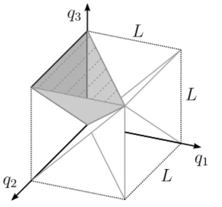
Figure 1: Fundamental domain F for N = 3, D = 1, bounded by symmetry planes q1 =q2 and q2 =q3 (light grey) and physical boundaries q1 = 0 and q3 =L (dark grey and shaded).
for the physical confinement to the line [0, L]. An example of this construction in the case of three fermions is shown in figure 1. The full domain can be reobtained by applying all possible permutationsP ∈SN to the fundamental domain
[0, L]N = [
P∈SN
P (F) . (24)
Due toD= 1, topological identification of boundary points in this context is not needed.
For fermions the restriction to antisymmetric states yields the condition of vanishing wave function all along the boundary
ψ(q) = 0 (∀q)(∃i6=j)(qi =qj). (25) As a Dirichlet boundary condition, this condition is sufficient to determine the eigenfunctions in F together with the single-particle conditions (23). The symmetry planes (22) can be thought of as hard walls or in other words infinite potential barriers.
The values of the wave functions in the other parts of the full domain are then obtained by
ψ(Pq) = (−1)Pψ(q) . (26) Thus a 1Dbilliard withN fermions is equivalent to a single-particle billiard of dimension N ·D, in which the usual Weyl expansion can be used to obtain ¯̺−(E).
One has to stress that this is a feature of one dimensional systems only because there no additional condition besides (25) is imposed on the wave function within the fundamental domain. In contrast to that, the corresponding condition ψ(q) = 0 for dimensions larger than one is not given along the whole boundaries of the fundamental domain, but instead only on lower dimensional manifolds embedded in those. The reason is that for D > 1, F is not bounded by the symmetry planes qi = qj, which have a dimension of N ·D−D < N ·D−1 and therefore are not able to separate volumes
in N ·D-dimensional configuration space. Rather the restriction to one of the spatial components in the conditions that define the symmetry planes are able to do so. One choice of fundamental domain is
F :=n
q∈ΩN
q1(1) ≤q2(1) ≤ · · · ≤q(1)N o
, (27)
where its symmetry related boundaries are defined through
qi(1) =qi+1(1) , i= 1, . . . , N −1, (28) and q ∈ ΩN denotes the physical confinement to the interior Ω ⊂ RD of the billiard.
The symmetry planes qi =qi+1, on which (26) imposes vanishing of the wave function, are only lower dimensional submanifolds embedded in the boundaries. Thus, the condition (26) can not be expressed as a Dirichlet boundary condition in a fundamental domain.
Moreover, even in the case of D = 1 sharp edges in the boundary of F can cause problems forN >2, making the expansion of Balian and Bloch [26] inapplicable, which is a generalization of the Weyl expansion to arbitrary dimensions but smooth boundaries.§ 5. Two Non-Interacting Fermions on a Line
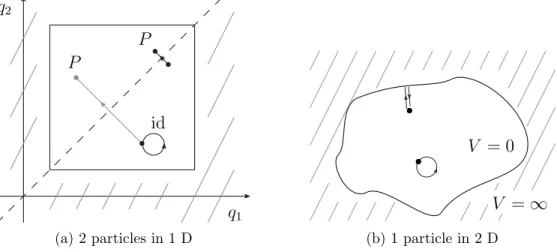
Consider a one-dimensional system of two fermions confined to a line of length L. The only two permutations are the identity and their exchange. Figure 2a illustrates the two possible contributions to the propagator. Since the system has an effective two- dimensional description it is straightforward to compare it to a single-particle two- dimensional billiard. There, ¯̺(E) is made up of contributions from free propagation and from reflections on the boundary, which is illustrated in figure 2b.
As discussed in section 4 there is a simple two-dimensional single particle billiard that is exactly equivalent to the two particle system. That is, the billiard defined by the fundamental domain, here chosen as F : L ≥ q1 ≥ q2 ≥ 0 with an additional hard wall boundary along the symmetry line q1 = q2. In this two-dimensional picture reflections on the additional boundary, which are addressed by propagation to mirror points, are mapped to the propagation with respect to the exchange permutation in the one dimensional many-body picture. Figure 3 illustrates the corresponding propagation in both pictures. The smooth part of the DOS of the two-fermion system including corner corrections reads
¯
̺−(E) =L2 8π
2m
~2
θ(E) − (2 +√ 2) L
8π 2m
~2 12
E−12θ(E) + 3
8δ(E). (29)
§ It is worth to note that one could topologically identify points along the boundary ofF that are related by symmetry and thereby create a fundamental domain with complex topology. We will call this object thewrapped fundamental domain. The problem in the fermionic case then would be the loss of continuity of the wavefunction because of sign inversionψ(q)→ −ψ(q) in the direction perpendicular to boundaries related to odd permutations. This condition seems quite peculiar and so far the author has not found a treatment of it in [26].
q1
id P
P
(a) 2 particles in 1 D
V = 0
V =∞
V = 0 V =∞
(b) 1 particle in 2 D
Figure 2: Comparison of the system of two identical particles in one dimension and one particle in two dimensions.
q1
q2
K(Pq,q;t)
(a) 2 particles in 1 D
q1
q2
K(Rq,q;t)
(b) 1 particle in 2 D
Figure 3: Equivalence of the system of two identical particles in one dimension and one particle in the two-dimensional fundamental domain.
The Weyl expansion (29) includes a volume term ¯̺v(E) with area A=L2/2, where the factor of 12 originating in the restriction to the fundamental domain corresponds to the factor 1/N! in the symmetry projected propagator (18). Thus this factor in the volume term, which corresponds to taking into account only the identity permutation, is the leading order effect of exchange symmetry. In general exchange corrections related to all other permutations are of sub-leading order as they correspond to Weyl-like boundary corrections. For example, in the case at hand, the only exchange permutation yields in leading order the perimeter correction proportional to √
2. Nevertheless, in general all exchange corrections are important to give physically reasonable results, as will be shown in the next sections.
6. General Case - Propagation in Cluster Zones
6.1. Invariant Manifolds and Cluster Zones
The last section showed that in the example of two particles on a line the correction to
¯
̺−(E) due to the exchange permutation is related to the propagation in the vicinity of the symmetry line q1 = q2 just as the inclusion of wave reflections in a single- particle billiard only affects the short time propagation near the physical boundary. The symmetry line is characterised by the invariance under P = ( 1 2 ), so that the distance
|Pq−q| becomes zero. This is the very reason to assume short path contributions to come from its vicinity. The concept of invariant manifolds is extended to the general case by finding the manifolds associated with each permutation P, defined by
MP =
q∈RN D
|Pq−q|= 0 ∩ΩN. (30) P can be written as a composition of commuting cycles (see for example [29])
P =σ1· · ·σl, (31) acting on distinct sets of particle indexes of size
N1, N2, . . . , Nl. (32) So we see that MP is the manifold defined by the coincidence of the coordinates of all particles associated with each cycle
MP =
\l
ω=1
q∈ΩN
qi =qj ∀i, j ∈Iω . (33) As a simple example take the permutation
P = ( 1 3 4 ) ( 2 5 ), (34)
whose associated manifold MP corresponds to the condition (see figure 4) q1 =q3 =q4
∧ q2 =q5
. (35)
In contrast to the symmetry line in the one-dimensional two particle case, these manifolds in general can not be seen as a boundary or surface in coordinate space in the sense of dividing the space into distinct pieces. The vicinities of these invariant manifolds shall from now on be referred to ascluster zones. All particles associated with a particular cycle index subset will be subsumed to the notion of a cluster. A system that is momentarily arranged in a particular cluster zone is composed ofl clusters, each associated with a cycle in P. Each cluster ω is composed of Nω particles according to the length of the cycle.
Figure 4: Example of the correspondence between the cycle decomposition of a permutation P and the invariant manifold MP pictured as the associated clustering of particles.
A separation into coordinates parallel toMP and perpendicular to it suggests itself, since the propagation near MP will not depend on shifting the position along them.
This holds at least as long as one does not get too close to the single-particle billiard boundaries to be included later. First, these single-particle boundary corrections shall be neglected, assuming the propagation to be invariant alongMP. This will be referred to as the unconfined case.
Furthermore, the invariance of propagation along the invariant manifolds is in a strict treatment also broken in the case of interaction. But the intention lying behind this construction is that when restricting to interactions of rather short range, the propagation can be assumed to be invariant along MP as long as one does not get too close to other invariant submanifolds. In other words, as long as the coordinates corresponding to different cycles do not become too close. Or to put it into a more intuitive picture, the different clusters should not collide. A discussion on that can be found in the last section.
6.2. The Measure of Invariant Manifolds
The infinitesimal volume element dµonMP is determined by the infinitesimal vectors in full (ND)-dimensional coordinate space lying inMP that correspond to the variations of independent coordinates.
First, for each permutation P in cycle decomposition (31–32) the particles are relabelled without loss of generality in a way that the first cycleσ1 involves the first N1 particles, the second cycle σ2 involves the N2 subsequent particles, and so on.
Since all particles associated with one cycle have to fulfil the condition of equal coordinates (33), there is exactly one independent D-dimensional vector for each cycle σω, ω = 1, . . . , l , while all other particles in the same cycle have to follow in order to remain on MP. Let the l independent vectors be denoted by
xω = (x(1)ω , . . . , x(D)ω )∈Ω, ω= 1, . . . , l . (36) With these preliminaries, any point on MP is described by
q= (x1, . . . ,x1
| {z }
N1
,x2, . . . ,x2
| {z }
N2
, . . . ,xl, . . . ,xl
| {z }
Nl
)∈ΩN. (37)
The infinitesimal volume element dµ ofMP is the volume of the parallelotope spanned by all l·D infinitesimal tangent vectors
∂q
∂x(d)ω
dx(d)ω , ω = 1, . . . , l, d= 1, . . . , D . (38) (dµ)2 equals the Gramian determinant Gof all these vectors, which is the determinant of the matrix made up of all pairwise scalar products. From (37) one obtains
∂q
∂x(d)ω
= (0, . . . ,0
| {z }
N1+···+Nω−1
,ed, . . . ,ed
| {z }
Nω
,0, . . . ,0
| {z }
Nω+1+···+Nl
) (39)
with
ed= (0, . . . ,0,1
↑ d−th
,0, . . . ,0)∈RD (40)
and therefore
* ∂q
∂x(d)ω
, ∂q
∂x(dω′′)
+
=δdd′δωω′Nω. (41)
The Gramian determinant reads G= det
diag(N1, . . . , N1
| {z }
D
, N2, . . . , N2
| {z }
D
, . . . , Nl, . . . , Nl
| {z }
D
)
·Yl
ω=1
dDxω
2
, (42)
dµ=√
G=p N1
D· · ·p Nl
D · dDx1 · · · dDxl. (43) The total measure of the manifold µ(MP) is obtained by integration of all independent coordinates xω over Ω:
µ(MP) = ˆ
dµ=VDl · Yl
ω=1
Nω
D2
, (44)
with the D-dimensional volume of the billiard VD =
ˆ
Ω
dDxω. (45)
This measure is only depending on the partition of N into integers N1 + · · · +Nl
corresponding to the decomposition of P into cycles with lengths N1, . . . , Nl. Each permutation associated with the particular partition {N1, . . . , Nl} yields an invariant manifold of the same measure (44). Furthermore the contributions from short path
relabelling particle indexes. This allows the replacement of the sum over all permutations by a sum over all distinct partitions of N with an additional factor of
c(N1, . . . , Nl) =N!Yl
ω=1
1 Nω
YN
n=1
1 mn!
(46)
in each summand, which is the number of permutations P ∈ SN with cycle lengths {N1, . . . , Nl} in their cycle decomposition. Thereby, mn denotes the multiplicity the cycle length n appears with.
7. The Weyl Expansion of Non-Interacting Particles
Up to this point, the analysis is quite general and is valid also for interacting systems.
Although we believe it to be feasible in the context of interaction, for now the non- interacting case will be carried out explicitly. Furthermore, in this calculation, effects of the physical boundary are omitted.
Under these assumptions the propagator in (18) is taken as the product of free propagators of all particles
K(q′,q;t) = YN
i=1
K0(q′i,qi;t). (47) At the end of this section, the full expression including effects of (locally flat) physical boundary can be found. The corresponding calculation is shown in the appendix.
For the calculation of the summand corresponding to a particular permutation P in (19), the particle indexes of different cycles inP don not mix up, yielding a product of independent propagators, which can be traced separately, each factor corresponding to a specific cycle in the decomposition (31). Consider now the trace of all coordinates corresponding to the cycle σω. For this purpose, the particles are relabelled, so that the indexes associated with σω are simply Iω = {1, . . . Nω}. For the sake of simplicity we write qand Pq by meaning the restrictions to the firstNω particles
q= (q1,q2, . . . ,qn),
Pq= (q2, . . . ,qn,q1). (48) Furthermore note the abbreviationn=Nω. The integral over the associated coordinates reads
ˆ
dnDq K0(Pq,q;t) = ˆ
dnDq m 2π~it
nD2
expi
~ m
2t|Pq−q|2
, (49)
where the equality of a product of n free propagators in D dimensions and one n·D- dimensional free propagator has been used. With the distance vector
Pq−q= (q2 −q1,q3−q2, . . . ,q1−qn), (50)
the squared distance is
|Pq−q|2 =|q2−q1|2+· · ·+|q1−qn|2
= XD
d=1
(q2(d)−q(d)1 )2+· · ·+ (q1(d)−q(d)n )2
. (51)
The overall squared distance is the sum of squared distances according to one spatial component, which are just the summands in (51). The following calculation proceeds in equal manner for all spatial components d = 1, . . . , D. So the notation is further simplified by calculating only the factor corresponding to one spatial component in (49) and by omitting the superscript (d). For this calculation in n-dimensional space we simply write q and Pq by meaning the corresponding tuples of one particular spatial component.
q= (q1, q2, q3, . . . , qn),
Pq= (q2, q3, . . . , qn, q1). (52) Which of the definitions (12), (48) and (52) is used in a particular step will be clear from the number of regarded dimensions in the context.
In this simplified notation (52) each summand in (51) is
|Pq−q|2 = (q2−q1)2+· · ·+ (qn−qn−1)2+ (q1−qn)2. (53) The trace to calculate is
ˆ
dnq K0(Pq,q;t) = ˆ
dnq m 2π~it
n2
expi
~ m
2t|Pq−q|2
. (54)
The squared distance is of second order in all coordinates, enabling to perform the integral (54) as a generalized multidimensional Gaussian integral
ˆ
dmx exp
−1
2xTMx
= s
(2π)m
det(M), M =MT ∈GLm, (55) which will not be used directly, since the determinant of M equals zero. It has one eigenvalue λ = 0 corresponding to the direction parallel to the invariant manifold, expressing the local translational invariance along
ˆ
qk = 1
√n(1, . . . ,1), (56)
since the distance vector is invariant in this direction,
P(q+aˆqk)−(q+aˆqk) = Pq−q + a(Pqˆk−qˆk
| {z }
= 0
) =Pq−q. (57)
to the invariant manifolds suggests itself. One way to proceed would be to introduce suitable perpendicular coordinates, perform the corresponding lower dimensional integral of the propagator and in the end multiply it by the measure of the invariant manifold. This would be the direct analogue to the usual computation of the surface correction in the single-particle Weyl expansion (15). One has to stress that in the interacting case this is most likely the most convenient way to calculate the trace of the propagator. And indeed, one can follow this procedure in the non-interacting case. But the introduction of perpendicular coordinates is rather uncomfortable since naturally one is lead to non-orthogonal coordinate systems and therefore has to introduce a metric tensor and pay extra attention to the arising volume elements. Although the calculation for the free case can be carried out in this manner, we will present an alternative approach in the non-interacting case that is more convenient and straightforward.
For the following analysis, a minimum cycle length of n ≥ 2 is assumed. The trivial case n = 1 will be included automatically in the resulting expressions. In the n-dimensional space of particle coordinates corresponding to only one cycle and only one spatial dimension, the subspace of vectors under which the squared distance is invariant is only one-dimensional (there is only one ˆqk). Accordingly, the matrix M has exactly one eigenvalue that is vanishing when bringing the trace (54) into the form of (55).
Therefore it is sufficient to separate one of the n coordinates, e.g. q1 and calculate the integral over all others as a generalized multidimensional Gaussian integral with linear term
ˆ
dmx exp
−1
2xTMx + vTx
= s
(2π)n
det(M) exp1
2vTM−1v
(58) with v ∈ Cm and M = MT ∈ GLm. The remaining integral ´
dq1 can then be kept and eventually, when considering all spatial components and cycles, it will automatically produce the measure of MP together with the determinant prefactors.
Parts of the prefactors will thereby act as the Jacobian determinant associated with the relation of the volume element of the manifold to the independent coordinates q1,ω(d) , d= 1, . . . , D , ω = 1, . . . , l. We abbreviate
α = i
~ m
2t (59)
and write (54) as
−α π
n2 ˆ
dq1exp 2αq12ˆ
dq2· · ·dqnexp
−α 2
Xn−1
i,j=1
Aijqi+1qj+1+α Xn−1
i=1
biqi+1
(60) with some symmetric matrix A and a vector b, which are identified by separating all
q1-dependent terms in (53):
|Pq−q|2 = 2q12+ Xn
i=2
2q2i − Xn−1
i=2
2qiqi+1
| {z }
=−12P
Aijqi+1qj+1
−2q1q2−2q1qn
| {z }
=P biqi+1
,
Aij =−4
δij − 1
2(δi,j+1+δi+1,j)
,
bi =−2q1(δi1+δi,n+1), i, j = 1, . . . , n−1.
(61)
A is a tridiagonal matrix of dimension n−1
A= (−4)·
1 −12 0 0 · · ·
−12 1 −12 0 · · · 0 −12 1 −12 0 0 −12 . .. ...
... ... . .. ...
, (62)
whose inverse and determinant are (A−1)ij =
( −12j(1− ni) i≥j
(A−1)ji i < j, , (63)
det(A) =n(−2)n−1. (64)
Using (61) and (63) gives
bTA−1b = 4q21[(A−1)11+ (A−1)1,n−1+ (A−1)n−1,1+ (A−1)n−1,n−1]
= 4q21
− 1 2n
[n−1 + 2 +n−1]
=−4q12.
(65)
With this and (58) the whole integral (60) becomes −α
π n2 s
(2π)n−1 αn−1det(A)
ˆ
dq1 exp
2αq12+1
2αbTA−1b
=
−α π
12 n−12
ˆ
dq1. (66)
By collecting all spatial components we get the contribution (49) corresponding to a particular cycle
ˆ
dnDq K0((Pq),q;t) =
−α π
D2 n−D2
ˆ
Ω
dDq1 = m 2π~it
D2 N−
D
ω 2VD, (67) where we reintroduced the notations (48) and n =Nω for the length of the particular cycle under investigation. Note that this general form also includes the case of a one- cycle Nω = 1.
one gets
ˆ
dN Dq K0((Pq),q;t) = m 2π~it
lD2 Yl
ω=1
Nω
−D2
VDl . (68) (68) as an expression associated with a permutationP only depends on the partition ofN into cycle lengths (as does the measureµ(MP) (44)). By collecting all permutations with the same partition in the sum overSN, the trace of the symmetry projected propagator can be written as
ˆ
dN Dq K0,±(q,q;t) = 1 N!
XN
l=1
(±1)N−l XN
N1,...,Nl=1 N1≤···≤Nl
δN,P
Nω c(N1, . . . , Nl)
× m 2π~it
lD2 Yl
ω=1
Nω
−D2
VDl .
(69)
As before,c(N1, . . . , Nl) denotes the number of permutations with a cycle decomposition of lengths N1, . . . , Nl (46). Using the bilateral Laplace transformation rule
L−1τ
Γ(ν) τν
(x) = 1 2πi
ˆ ǫ+i∞
ǫ−i∞
dτ Γ(ν)
τν eτ x =xν−1θ(x), ν > 0, (70) with the Heaviside step function θ(x), the final result for the smooth part of the symmetry projected DOS (19) for a system ofN identical non-interacting bosons (+) or fermions (−) in a D-dimensional billiard of volumeVD without confinement corrections reads
¯
̺±(E) = 1 N!
XN
l=1
(±1)N−l
XN
N1,...,Nl=1 N1≤···≤Nl
δN,P
Nω c(N1, . . . , Nl)Yl
ω=1
1 Nω
D2
× m 2π~2
lD2 VDl
Γ lD2 ElD2 −1θ(E).
(71)
In general (71) is a sum of powers of E with coefficients that are, besides their dependence on the billiard volume, expressed as sums over partitionsN =N1+· · ·+Nl
only depending onN, l and Dand therefore universal for allN-particle billiard systems with dimension D. A more compact form of (71) can be obtained by appropriately scaling the density and energy and rewriting the sum over partitions as ordered tuples.
Using (46) and defining the scaling-density
̺0 = mD√ VD
2
2π~2 ⇔ ̺¯sp(E) =̺0
(̺0E)D2−1
Γ D2 , (72)
which is roughly the density at the first single-particle level, and the universal coefficients Cl=
XN
N1,...,Nl=1 PNω=N
Yl
ω=1
1 Nω
D2+1
, (73)
leads to
¯
̺±(E) =̺0
XN
l=1
(±1)N−l l! Cl
(̺0E)lD2 −1
Γ lD2 θ(E). (74)
An extension of (74) is given by the inclusion of physical boundary effects. Its derivation under the assumption of locally flat boundaries can be performed directly by incorporating the additional geometrical features to the propagation in cluster zones. But as this way to proceed gets extensive and seems a bit long-winded, an alternative, indirect but equivalent derivation utilizing a convolution formula (82) by Weidenm¨uller [21] is chosen for this publication and can be found in Appendix C. The resulting expression reads
¯
̺±(E) =̺0
XN
l=1
(±1)N−l Xl
lV,lS=0 Pli=l
Cl,lVγlS lV!lS!
(̺0E)λ−1
Γ(λ) θ(E), (75)
where λ=lVD/2 +lS(D−1)/2. It depends on the universal coefficients Cl,lV =
XN
N1,...,Nl=1 PNω=N
YlV
ω=1
1 Nω
D2+1 Yl
ω=lV+1
1 Nω
D2+21
, (76)
and the dimensionless geometrical parameter γ =± SD−1
4D√ VD
D−1 , (77)
which represents the ratio of the surface SD−1 to the volume VD of the billiard. The plus(minus) sign in (77) refers to van Neumann(Dirichlet) conditions at the physical boundary. Equations (74) and (75) can be regarded as the main results of this publication. lV+lS =l represents the splitting of all lclusters into such that contribute via free propagation in the interior (lV) and such that contribute by reflection along the boundary (lS) of the billiard. In the case of D = 1 the summands corresponding to lV = 0 have to be replaced according to the rule
(̺0E)lS(D2−1)−1
Γ lS(D−1)2 θ(E)D→1−→ δ(̺0E) (78)
and in (77) the surfaceS0 has to be taken as the number of bordering end-points, which would be two for a finite line and zero for the one-sphere-topology. The unconfined
Cl,lV=l =Cl.
The highest power of the energy in (74,75) has the exponent (ND)/2−1, which reminds of the Thomas-Fermi approximation of the effectivelyN·D-dimensional billiard.
This is not surprising, since l = N refers to a partition into unities N = 1 +· · ·+ 1 associated solely with the identity permutation P = idSN = ( 1 ) ( 2 )· · · (N). In the geometrical picture, this corresponds to the propagation of individual particles. None of them are clustered and in (75) none of them are reflected on the boundary, since lS = 0 for the highest power. The combinatorial factor (46) and the coefficients (73) and (76) compute to c(1, . . . ,1) = CN =CN,N = 1 and the corresponding term in (71), (74) and (75) is the volume Weyl term of the fundamental domain inN·D-dimensional space
¯
̺v(E) = 1 N!̺
N D
02
EN D2 −1 Γ N D2 θ(E)
= 1 N!
m 2π~2
N D2 VDN
Γ N D2 EN D2 −1θ(E)
= 1
N!̺¯TF(E).
(79)
The next section will show the importance of all corrections in (71), (74) and (75) beyond the volume term (79).
8. The Geometrical Emergence of Ground State Energies in Fermionic Systems
As often in the context of semiclassics the case of a two-dimensional billiard is of special interest. On the one hand, this is because of possible technical applications. One can think of confined two-dimensional electron gases in semiconductor heterostructures or two-dimensional superconducting structures with bosonic description due to Cooper pairing for example. On the other hand, the existence of equally distributed energies in a 2Dsingle-particle billiard without boundary corrections is a valuable special feature.
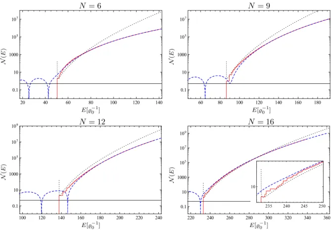
This is not only because of the exceptionally simple form that the density of states takes in these systems. A constant single-particle smooth part also opens the possibility to make connections to number theory. Namely approximations for average distributions of partitions of integers can be related.
For positive arguments E the unconfined DOS (74) in D = 2 is a polynomial of degree N −1 in the energy with coefficients that are just rational numbers. The coefficients can be summed up exactly for explicit values of N and l albeit with computation time increasing very strongly with N when using the form at hand (71) or (74). Note that the form of the coefficients used in (71) in terms of ordered partitions corresponds to less computation time while the form (74) seems to be a better starting point for simplifications or analytical calculations.