Quantum Mechanics 1 Lecture 10: Spin and addition of angular momenta

Quantum Mechanics 1

Lecture 10: Spin and addition of angular momenta

Massimiliano Grazzini

University of Zurich

Outline

Addition of angular momenta Spin

Back to angular momentum

- Wigner-Eckart theorem

- Anomalous Zeeman effect

- addition of two 1/2 spins

Back to angular momentum

In Lecture 6 we have seen that the condition that the angular momentum wave functions take the same value when the azimuthal angle

implies that the quantum number must be integer

ψ

_lm

(θ, ϕ)

ϕ → ϕ + 2π l

The angular momentum realised on single-valued functions of the coordinates is called orbital angular momentum

In this case the angular momentum algebra is realised on the infinite dimensional Hilbert space and the rotation is realised through generators that take the form of differential operators ^L

2

(S

₂

)

But if, for example, we consider a vector we can study the effect of rotations on the space corresponding to the index ^v

^j

^{( j = 1,2,3)} _j

In this case we are considering the action of a rotation on a finite dimensional space and (recall MMP2) the generators are realised as finite dimensional

matrices on such space

θ ϕ

x

x

₁

x₂ x₃

The angular momentum algebra

[J

_i

, J

_j

] = iℏϵ

_ijk

J

_k

Is now realised on the 3-dimensional space for which a basis can be chosen as

u

₁

= (

1 0

0 ) u

₂

= (

0 1

0 ) u

₃

= (

0 0 1 )

(1)

Note that in Eq. we have replaced (which is normally used to denote orbital angular momentum) with ⁽¹⁾ _J

_i

^L

ⁱ

If we choose a vector _{v =}

(

cos α sin α

0 )

and we do a rotation of an angle around the 3 axis we find _δϕ

v′ = R

₃

(δϕ)v = cos(α + δϕ) sin(α + δϕ)

0

= cos α − δϕ sin α sin α + δϕ cos α

0

This can be rewritten as

v′ = ( 1 − i

ℏ δϕ J

₃

) v where

J

₃

= − iℏ (

0 1 0

− 1 0 0 0 0 0 )

We can extend this to rotations around the and axes to find _{x y} J

₁

= − iℏ

(

0 0 0 0 0 1

0 − 1 0 ) J

₂

= − iℏ (

0 0 − 1 0 0 0 1 0 0 ) And check that the generators fulfil the algebra in Eq. ₍₁₎

By repeating the steps done in Lecture 6 we find that _{j = 1} and that _{m = − 1,0,1} We have constructed a finite-dimensional spin-1 representation of the angular momentum algebra (recall the discussion of finite dimensional representations of

in MMP2)

SO(3)

Spin

In Lecture 9 we have seen that for an electron in a magnetic field the interaction is

H

_int

= − e

2mc B ⋅ L = − μ ⋅ B

where _{μ =} ^e

2mc L

The quantity _{e /(2mc)} is called gyromagnetic ratio

This interaction splits the _{2l + 1} angular momentum eigenstates by the quantity

μ

_B

Bm

_l

with _μ

_B

₌ ^{| e | ℏ}

2mc Bohr magneton

m

_l

= − l, . . . . . l

Experimentally however the splitting for atoms with odd atomic number is what

one would have if where half-integer and the splitting depends on the level _m

_l

^Z

Stern-Gerlach experiment

An atomic beam passes

through an inhomogeneous magnetic field

The experiment was carried out in 1922 by using silver atoms

Silver has a spherically

symmetric charge distribution plus an electron in a 5s orbital

Therefore the total angular momentum is vanishing, i.e. and there should be

no splitting ^{l = 0}

The experiment, however, shows a splitting in two beams

The electron must have an intrinsic angular momentum, called spin, with a corresponding gyromagnetic ratio _{e / mc}

The electron spin can only be _{+ ℏ /2} or _{−ℏ /2} in a arbitrary chosen direction

z

magnet

Spin 1/2

Let us denote by the spin operator _S

According to the previous discussion if is an arbitrary direction we must have _n

S ⋅ n | n, ± ⟩ = ± ℏ

2 | n, ± ⟩

If we choose along the axis we have _{n z}

S

₃

| ± ⟩ = ± ℏ

2 | ± ⟩

and in this basis takes the form _S

₃

S

₃

= ℏ

2 ( 1 0 0 − 1 )

The vectors and correspond to different eigenvalues of the Hermitian operator and are thus orthonormal _S

₃

^{| + ⟩ | − ⟩}

⟨ + | − ⟩ = ⟨ − | + ⟩ = 0 ⟨ + | + ⟩ = ⟨ − | − ⟩ = 1

[S

_i

, S

_j

] = iℏϵ

_ijk

S

_k

By using the commutation relations

we can define the _S

_±

_{= S}

₁

± iS

₂

operators and we find j = 1/2 and m = ± 1/2

S

₋

| − ⟩ = S

₊

| + ⟩ = 0 S

₋

| + ⟩ = | − ⟩ S

₊

| − ⟩ = | + ⟩

The operators and can be represented as _S

₊

_S

₋

S

₊

= ℏ ( 0 1

0 0 ) S

₋

= ℏ ( 0 0 1 0 )

Introducing the Pauli matrices

σ

₁

= ( 0 1

1 0 ) σ

₂

= ( 0 − i

i 0 ) σ

₃

= ( 1 0 0 − 1 )

We can write _{S =} ^ℏ

2 σ

The Pauli matrices have the properties

σ

₁²

= σ

₂²

= σ

₃²

= I [σ

_i

, σ

_j

] = 2iϵ

_ijk

σ

_k

{σ

_i

, σ

_j

} = 2δ

_ij

I Tr [ σ

_i

] = 0

In the basis we are using a general spin state can be written as

| χ⟩ = α | + ⟩ + β | − ⟩ with _{α, β ∈ ℂ} and _{| α |}

²

_{+ | β |}

²

_{= 1} we can of course write

α = ⟨ + | χ⟩ β = ⟨ − | χ⟩

This general state can also be represented as a two-component vector

χ = ( α β )

This vector is known as spinor

It is an example of a two-level quantum system called also qubit, the

basic unit of quantum information

Suppose we have an electron with spin aligned in the direction, that is in a state _z

| χ⟩ = | + ⟩

We ask the following question: what is the probability that a measurement of the spin in the direction gives _x ± ℏ /2 ?

S

₁

= ℏ

2 ( 0 1 1 0 )

The eigenvectors of

are _u

1+

= 1

2 ( 1

1 ) ^u

¹⁻

^{= 1} ₂ ( − 1

1 )

with _S

1

u

₁₊

= + ℏ

2 u

₁₊

S

₁

u

₁₋

= − ℏ 2 u

₁₋

The state _{| χ⟩} can be written as

| χ⟩ = | + ⟩ = 1

2 | u

₁₊

⟩ − 1

2 | u

₁₋

⟩

The probabilities to obtain _{+ ℏ /2} or _{−ℏ /2} are equal to _1/2

More generally we can ask the question: what is the probability that in the state a measurement of the spin in an arbitrary direction gives ?

| χ⟩ = | + ⟩ n ± ℏ /2

The operator _{S ⋅ n} can be written as

S ⋅ n = ℏ

2 σ ⋅ n

By using spherical coordinates can be written as _n

n = (sin θ cos ϕ, sin θ sin ϕ, cos θ) θ ϕ

x

x

₁

x₂ x₃

= ℏ

2 ( cos ϕ sin θ ( 0 1

1 0 ) + sin ϕ sin θ ( 0 − i

i 0 ) + cos θ ( 1 0

0 − 1 ) )

= ℏ

2 ( cos θ sin θe

^−iϕ

sin θe

^iϕ

− cos θ )

Its eigenvectors are

u

_n+

= ( cos (θ /2)

sin (θ /2) e

^iϕ

) u

_n−

= ( − sin (θ /2) e

^−iϕ

cos (θ /2) )

with _{(S ⋅ n)u}

_n±

_{= ±} ^ℏ

2 u

_n±

An arbitrary normalised spin state _{| χ⟩} can be written as

| χ⟩ = a

₊

| + ⟩ + a

₋

| − ⟩ with _{| a}

₊

_|

²

_{+ | a}

₋

_|

²

_{= 1}

Since the overall phase is irrelevant we can choose the following parametrisation for and _a

₊

_a

₋

| χ⟩ = cos(θ /2) | + ⟩ + e

^iϕ

sin(θ/2) | − ⟩ with _{0 ≤ θ ≤ π} and _{0 ≤ ϕ ≤ 2π} Therefore the probability that in the state a measurement of the spin in the direction gives the result is

| χ⟩ = | + ⟩

n ± ℏ

2

P

_n,+

= | ⟨ χ | u

_n+

⟩ |

²

= cos

²

(θ /2) P

_n,−

= | ⟨ χ | u

_n−

⟩ |

²

= sin

²

(θ/2)

We now want to give an interpretation to the matrix element when

is an arbitrary state ^{⟨ χ | S | χ⟩ | χ⟩}

Therefore the vector

⟨ χ | S | χ⟩ = ℏ

2 (cos ϕ sin θ, sin ϕ sin θ, cos θ) θ ϕ

| χ⟩

x

₁

x₂ x₃

maps out a sphere called Bloch sphere with the corresponding angles and _{θ ϕ}

More generally the Bloch sphere is a geometrical representation of the pure state space of a two-level quantum mechanical system

| + ⟩

| − ⟩

If we compute the expectation value of the spin operator _{⟨ χ | S | χ⟩} we find

⟨ χ | S

₁

| χ⟩ = ℏ

2 ( cos (θ/2)

sin (θ/2) e

^−iϕ

) ( 0 1

1 0 ) ( cos (θ/2)

sin (θ/2) e

^iϕ

) = ℏ

2 cos ϕ sin θ

⟨ χ | S

₂

| χ⟩ = ℏ

2 ( cos (θ/2)

sin (θ/2) e

^−iϕ

) ( 0 − i

i 0 ) ( cos (θ/2)

sin (θ/2) e

^iϕ

) = ℏ

2 sin ϕ sin θ

⟨ χ | S

₃

| χ⟩ = ℏ

2 ( cos (θ/2)

sin (θ/2) e

^−iϕ

) ( 1 0

0 − 1 ) ( cos (θ/2)

sin (θ/2) e

^iϕ

) = ℏ

2 cos θ

Magnetic moment

μ

_orbit

= e

2mc L

We have seen in Lecture 9 that a magnetic moment

is associated with the orbital angular momentum of an electron _L

There is no reason to expect that the magnetic moment due to the spin should have the same ratio to as the one for the orbital angular momentum _S

We can write

μ

_spin

= g e 2mc S

Where is the gyromagnetic factor _g

The relativistic theory (through the Dirac equation) predicts

g = 2

Radiative corrections in the quantum theory of electromagnetism (QED) correct this value to

g = 2 ( 1 + α

2π + . . . . ) = 2.0023...

This comes from the term ₋ ^e in the Hamiltonian

2mc (L ⋅ B) = − μ

_orbit

⋅ B

The total magnetic moment is thus to a very good approximation

μ = μ

_orbit

+ μ

_spin

= − e

2mc (L + 2S)

and we now need to understand how to add angular momenta

For the proton and the neutron, the magnetic moment is usually expressed in units of the nuclear magneton

for protons

g = 5.59 _{g = − 3.83} for neutrons

where _m

_N

_{∼ m}

_p

_{∼ m}

_n

_{∼ 940 MeV/ c}

²

We see that the neutron has a magnetic moment despite the fact that is neutral:

this means that it cannot be an elementary particle

μ

_N

= | e | ℏ 2m

_N

c

Experimentally we find We define

μ = gμ

_N

S

Spin and magnetic moment are always opposite !

Note that also neutral composite particles like , , have a magnetic moment,

which arises from their internal charge distribution ^{n Λ Σ}

⁰

Addition of angular momenta

A central problem in Quantum Mechanics is the one of combining angular momenta of two parts of a system, such as:

orbital angular momenta of two electrons in an atom

spin and orbital angular momentum of the same electron

The magnitude of the sum of two angular momenta and can have any value ranging from the sum of their magnitudes (parallel case) to the difference of their magnitude (antiparallel case)

J

_a

J

_b

The sum of the -components of the angular momenta equals that of their resultant ^z

We will now see that both these rules hold in Quantum Mechanics as well

At the classical level the problem is solved by using the vector addition rule:

We consider two angular momentum operators and that correspond to distinct degrees of freedom, and, therefore, commute ^J

^a

^J

^b

[J

_a

, J

_b

] = 0

Both and satisfy the angular momentum algebra _J

_a

_J

_b

[J

_a,i

, J

_a,j

] = iϵ

_ijk

J

_a,k

[J

_b,i

, J

_b,j

] = iϵ

_ijk

J

_b,k

The orthonormal eigenstates of and _J

²_a

_J

_a,3

are _{| j}

_a

_{, m}

_a

_⟩ and has no effect on them _J

_b

Analogously, _{| j}

_b

_{, m}

_b

_⟩ are the eigenstates of and _J

²_b

_J

_b,3

and has no effect on them _J

_a

The direct product representation (recall MMP2) is specified by the vectors

| j

_a

m

_a

; j

_b

m

_b

⟩ = | j

_a

m

_a

⟩ × | j

_b

m

_b

⟩

Since and commute, also the total angular momentum fulfils the angular momentum algebra ^J

^a

^J

^b

^{J = J}

^a

^{+ J}

^b

[J

_i

, J

_j

] = iϵ

_ijk

J

_k

The orthonormal states of and are denoted by and identify another

representation ^J

2

J

₃

| jm⟩

We would like to find the unitary transformation relating the two representations However, we do not need to deal with the infinite-dimensional Hilbert space at once: we can focus on the subspace in which and have definite values _j

_a

_j

_b

The dimensionality of this subspace is _(2j

_a

_{+ 1)(2j}

_b

_{+ 1)} We can write

_{|jm⟩ = | j}

am_a; j_bm_b⟩⟨j_am_a; j_bm_b|jm⟩

Where a summation over from _m

_a

_{− j}

_a

to and over from _j

_a

_m

_b

_{− j}

_b

to is understood _j

_b

m = m

_a

+ m

_b

The coefficients _{⟨ j}

_a

_m

_a

_{; j}

_b

_m

_b

_{| jm⟩} are called Clebsch-Gordan coefficients

We first observe that since the coefficient must vanish unless ^J

³

^{= J}

^a,3

^{+ J}

^b,3

^{⟨ j}

^a

^m

^a

^{; j}

^b

^m

^b

^{| jm⟩}

This means that the maximum value of is and that this occurs only once, when _m

_a

_{= j}

_a

and _m

_b

_{= j}

_b

^{m j}

^a

^{+ j}

^b

Therefore the maximum value of is _{j j = j}

_a

_{+ j}

_b

and there is only one such state

We have

_{|j = j}

a + j_b, m = j_a + j_b⟩ = |j_aj_a; j_bj_b⟩

The next largest value of is and it occurs twice: when and or when ^{m j} and

^a

^{+ j}

^b

^{− 1 m}

^a

^{= j}

^a

m

_b

= j

_b

− 1 m

_a

= j

_a

− 1 m

_b

= j

_b

One of the two linearly independent combinations of these two states must be

associated with a state for which since for that there must exist values of

ranging from to ^{j = j}

^a

^{+ j}

^b

^j

m j

_a

+ j

_b

− j

_a

− j

_b

Recalling that

J

₋

| jm⟩ = j( j + 1) − m(m − 1) | j, m − 1⟩

we can explicitly construct such state by applying _J

₋

_{= J}

_a,−

_{+ J}

_b,−

on _{| j}

_a

_{+ j}

_b

_{, j}

_a

_{+ j}

_b

_⟩

| j

_a

+ j

_b

, j

_a

+ j

_b

− 1⟩ = 1

2( j

_a

+ j

_b

) J

₋

| j

_a

+ j

_b

, j

_a

+ j

_b

⟩ = 1

2( j

_a

+ j

_b

) (J

_a,−

+ J

_b,−

) | j

_a

j

_a

; j

_b

j

_b

⟩

= 2j

_a

2( j

_a

+ j

_b

) | j

_a

, j

_a

− 1; j

_b

, j

_b

⟩ + 2j

_b

2( j

_a

+ j

_b

) | j

_a

, j

_a

; j

_b

, j

_b

− 1⟩

We have _J

₋

_{| jj⟩ = 2j | j, j − 1⟩}

The other combination must be associated to and should be orthogonal to the previous one, so, up to a phase, it must take the form ^{j = j}

^a

^{+ j}

^b

^{− 1}

| j

_a

+ j

_b

− 1,m

_a

+ m

_b

− 1⟩ = − j

_b

j

_a

+ j

_b

| j

_a

, j

_a

− 1; j

_b

, j

_b

⟩ + j

_a

j

_a

+ j

_b

| j

_a

, j

_a

; j

_b

, j

_b

− 1⟩

We can now go on applying to construct the remaining states _J

₋

Proceeding in this way we span all the values of from to and for each of them we have _{(2j + 1)} states, so the total number of states is ^{j j}

^a

^{+ j}

^b

^{| j}

^a

^{− j}

^b

^|

j_a+j_b j=|

∑

j_a−j_b|

(2j + 1) = ∑

^2jb

k=0

(2( j

_a

− j

_b

) + 2k + 1) = ( 2( j

_a

− j

_b

) + 1 ) (2j

_b

+ 1) + 2 ∑

^2jb

k=0

k

Consistently with what was expected

We have decomposed the direct product representation in the sum of irreducible representations

𝒟

_ja

⊗ 𝒟

_jb

= ⨁

^ja+jb

j=|j −j |

𝒟

_j

= (2j

_a

+ 1)(2j

_b

+ 1)

^{(2jb)(2jb + 1)/2} assume for example

and set _{j = ja − jb + k} ^{ja > jb}

Example: addition of two 1/2 spins

In the case _j

_a

_{= 1/2} and _j

_b

_{= 1/2} the possible values of are _{j j = 0} and _{j = 1}

| 1,1⟩ = | 1 2 , 1

2 ⟩ × | 1 2 , 1

2 ⟩ = | + ⟩ | + ⟩

| 1,0⟩ = 1

2 ( J

_a−

+ J

_b−

) | 1

2 , 1 2 ⟩ × | 1

2 , 1 2 ⟩ = 1

2 | 1

2 , − 1

2 ⟩ × | 1

2 , 1 2 ⟩ + 1

2 | 1

2 , 1 2 ⟩ × | 1

2 , − 1 2 ⟩

= 1 2 ( | − ⟩ | + ⟩ + | + ⟩ | − ⟩ )

|1, − 1⟩ = | 1

2, − 1

2⟩ × | 1

2, − 1

2⟩ = | − ⟩| − ⟩

The state _{| 0,0⟩} can be obtained by requiring it to be orthogonal to _{| 1,0⟩}

| 0,0⟩ = 1

2 ( | − ⟩ | + ⟩ − | + ⟩ | − ⟩ )

triplet

singlet

34. Clebsch-Gordan coefficients 010001-1

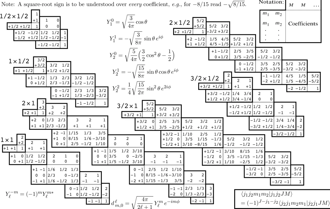
34. CLEBSCH-GORDAN COEFFICIENTS, SPHERICAL HARMONICS, AND d FUNCTIONS

Note: A square-root sign is to be understood over every coefficient, e.g., for −8/15 read −!

8/15.

Y₁⁰ =

"

3

4π cosθ Y₁¹ =−

"

3

8π sinθe^iφ Y₂⁰ =

"

5 4π

#3

2 cos²θ− 1 2

$

Y₂¹ = −

"

15

8π sinθcosθe^iφ Y₂² = 1

4

"

15

2π sin²θe^2iφ

Y_"^−m = (−1)^mY_"^m∗ "j₁j₂m₁m₂|j₁j₂JM#

= (−1)^J−j1−j2"j₂j₁m₂m₁|j₂j₁JM#

d^"_m,0 =

"

4π

2#+ 1 Y_"^me^−imφ

d^j_m!,m = (−1)^m−m!d^j_m,m! = d^j

−m,−m^! d¹_0,0 = cosθ d^1/2_1/2,1/2 = cos θ

2 d^1/2_1/2,

−1/2 = −sin θ 2

d¹_1,1 = 1 + cosθ 2 d¹_1,0 = −sinθ

√2 d¹_1,−1 = 1 −cosθ

2

d^3/2_3/2,3/2 = 1 + cosθ

2 cos θ 2 d^3/2_3/2,1/2 =−√

31 + cosθ

2 sin θ 2 d^3/2_3/2,

−1/2 = √

31−cosθ

2 cos θ 2 d^3/2_3/2,−3/2 = −1−cosθ

2 sin θ 2 d^3/2_1/2,1/2 = 3 cosθ−1

2 cos θ 2 d^3/2_1/2,−1/2 = −3 cosθ + 1

2 sin θ 2

d²_2,2 = #1 + cosθ 2

$₂

d²_2,1 = −1 + cosθ 2 sinθ d²_2,0 =

√6

4 sin²θ d²_2,−1 = −1−cosθ

2 sinθ d²_2,−2 = #1−cosθ

2

$₂

d²_1,1 = 1 + cosθ

2 (2 cosθ −1) d²_1,0 = −

"

3

2 sinθ cosθ d²_1,−1 = 1−cosθ

2 (2 cosθ + 1) d²_0,0 = #3

2 cos²θ− 1 2

$

+1

5/2 5/2

+3/2 3/2 +^3/2 1/5 4/5

4/5

−1/5 5/2

5/2

−^1/2 3/5 2/5

−1

−² 3/2

−^1/2

2/5 5/2 3/2

−3/2

−3/2 4/5

1/5 −4/5 1/5

−1/2

−2 1

−5/2 5/2

−3/5

−1/2 +1/2 +¹−^{1/2 2/5 3/5}

−^2/5

−1/2 2

+² +^3/2 +^3/2

5/2

+^{5/2 5/2}

5/2 3/2 1/2 1/2

−^1/3

−¹ +1 0 1/6 +1/2

+1/2

−1/2

−3/2 +1/2

2/5 1/15

−^8/15 +1/2

1/10 3/10

3/5 5/2 3/2 1/2

−^1/2 1/6

−1/3 5/2

5/2

−5/2 1 3/2

−3/2

−3/5 2/5

−3/2

−3/2 3/5 2/5 1/2

−1

−1 0

−^1/2 8/15

−1/15

−2/5

−1/2

−3/2

−^1/2 3/10 3/5 1/10 +3/2

+3/2 +^1/2

−^1/2 +3/2

+1/2 +2+1

+²

+¹ +⁰1

2/5 3/5

3/2 3/5

−2/5

−1 +¹ 0 +3/2 +1 1

+3

+¹ 1 0

3 1/3 +² 2/3

2 3/2

3/2 1/3 2/3 +1/2

0

−¹ 1/2 +1/2 2/3

−^1/3

−^1/2 +1/2 1

+^{1 1} 0 1/2 1/2

−1/2 0 0 1/2

−1/2 1 1

−¹

−^1/2 1

1

−1/2 +^1/2 +1/2+1/2

+1/2

−1/2

−1/2

+1/2 −1/2

−1 3/2

2/3 3/2

−3/2 1 1/3

−1/2

−1/2 1/2 1/3

−2/3 +1 +1/2

+1 0

+^3/2

2/3 3

3

3

3

3

−1 1

−2

−3 2/3

1/3

−2 2 1/3

−2/3

−2 0

−1

−2

−¹ 0 +1

−¹ 2/5 8/15 1/15

2

−¹

−¹

−2

−¹ 0 1/2

−1/6

−1/3

1

−¹ 1/10

−3/10 3/5 0

2 0

1 0 3/10

−^2/5 3/10 0

1/2

−^1/2 1/5 1/5 3/5 +¹

+1

−¹ 0 0

−1 +¹ 1/15

8/15 2/5

2

+^{2 2} +1 1/2 1/2

1 1/2 2

0 1/6 1/6 2/3

1 1/2

−1/2 0

0 2

2

−²

−1 1

−1 1

−1 1/2

−^1/2

−1 1/2 1/2 0 0

0

−¹ 1/3 1/3

−^1/3

−1/2 +1

−¹

−¹ 0 +¹

0 0

+1

−1 2

1 0 0 +1 +1 +1

+¹ 1/3 1/6

−1/2

1 +¹ 3/5

−3/10 1/10

−1/3

−1 +1 0

0 +²

+1 +2 3

+3/2

+1/2 +¹

1/4 2

2

−¹ 1

2

−² 1

−¹ 1/4

−1/2 1/2

1/2

−^1/2 −^1/2 +^1/2

−^3/2

−3/2 1/2

1 0 0 3/4

+1/2

−^1/2 −^1/2

2 +¹ 3/4

3/4

−^3/4 1/4

−1/2 +^1/2

−1/4 1

+1/2

−^1/2 +1/2 1

+1/2 3/5

0

−1 +^1/2

0

+1/2

3/2 +1/2 +^5/2

+² −^1/2 +2 +1/2

+1 +1/2 1

2×1/2

3/2×1/2

3/2×1 2×1

1×1/2 1/2×1/2

1×1

Notation: ^{J J}

M M

...

...

.. . ..

.

m₁ m₂

m₁ m₂ Coefficients

−^1/5

2 2/7 2/7

−3/7 3 1/2

−1/2

−1

−2 −2

−1

0 4

1/2 1/2

−3 3 1/2

−^1/2

−2 1

−44

−2 1/5

−^27/70 +^1/2

7/2 +7/2 7/2

+5/2 3/7 4/7 +2 +1 0 1 +2 +1

+4 1

4

4 +² 3/14 3/14 4/7

+² 1/2

−^1/2 0

+²

−1 0 +1 +2 +2 +¹ 0

−1

3 2

4 1/14 1/14 3/7 3/7 +¹

3

1/5

−^1/5 3/10

−3/10 +¹

2

+² +¹ 0

−¹

−2

−²

−¹ 0 +1 +2 3/7 3/7

−^1/14

−^1/14 +¹

1

4 3 2

2/7

2/7

−^2/7 1/14

1/14 4

1/14 1/14 3/7 3/7

3 3/10

−^3/10 1/5

−^1/5

−1

−²

−2

−1 0 0

−1

−2

−1 0 +1 +¹

0

−¹

−²

−1

2

4 3/14 3/14 4/7

−² −² −² 3/7

3/7

−1/14

−^1/14

−1

1 1/5

−3/10 3/10

−1

1 0

0 1/70

1/70 8/35 18/35 8/35

0 1/10

−1/10 2/5

−^2/5 0

0 0

0 2/5

−2/5

−^1/10 1/10

0 1/5 1/5

−^1/5

−^1/5 1/5

−1/5

−^3/10 3/10 +¹ 2/7

2/7

−3/7 +3

1/2 +² +1 0 1/2 +2 +2

+² +¹ +²

+¹

+3 1/2

−^1/2 0 +1 +2 3 4

+1/2 +3/2 +3/2

+2 +5/2

4/7 7/2 +3/2 1/7 4/7 2/7

5/2 +3/2

+² +1

−¹ 0 16/35

−^18/35 1/35

1/35 12/35 18/35 4/35 3/2

+3/2 +3/2

−^3/2

−1/2 +1/2 2/5

−2/5 7/2

7/2 4/35 18/35 12/35 1/35

−^1/2

5/2 27/70 3/35

−5/14

−6/35

−^1/2 3/2

7/2

7/2

−^5/2 4/7 3/7

5/2

−^5/2 3/7

−4/7

−3/2

−2 2/7

4/7 1/7

5/2

−3/2

−1

−2 18/35

−1/35

−^16/35

−3/2 1/5

−2/5 2/5

−3/2

−1/2 3/2

−3/2

7/2 1

−7/2

−^1/2 2/5

−1/5 0 0

−1

−² 2/5

1/2

−^1/2 1/10 3/10

−1/5

−^2/5

−3/2

−1/2

+1/2 5/2 3/2 1/2

+^1/2 2/5 1/5

−3/2

−1/2 +1/2 +3/2

−^1/10

−3/10 +^1/2

2/5 2/5 +1

0

−1

−2 0 +³³ 3 +²

2 +² +^3/2 1

+^3/2 +^1/2

+^{1/2 1/2}

−^1/2

−^1/2 +1/2 +3/2

1/2 3 2

3 0 1/20 1/20 9/209/20

2 1

3

−1 1/5 1/5 3/5

2

3

3 1

−³

−² 1/2 1/2

−3/2 2 1/2

−1/2

−3/2

−²

−1 1/2

−^1/2

−1/2

−^3/2 0

1

−1 3/10 3/10−2/5

−3/2

−1/2 0

0 1/4 1/4

−1/4

−1/4

0 9/20 9/20 +^1/2

−1/2

−^3/2

−1/20

−1/20 0 1/4

−1/41/4

−1/4

−^3/2

−1/2 +^1/2 1/2

−1/2 0

1 3/10 3/10

−3/2

−^1/2 +^1/2 +^3/2 +3/2

+^1/2

−^1/2

−^3/2

−2/5 +¹ +¹

+¹ 1/5 3/5 1/5 1/2

+^3/2 +1/2

−1/2 +^3/2 +^3/2

−^1/5 +^1/2 6/35 5/14

−^3/35 1/5

−3/7

−1/2 +1/2 +3/2

2×3/2 5/2

2×2

3/2×3/2

−3

Figure 34.1: The sign convention is that of Wigner (Group Theory, Academic Press, New York, 1959), also used by Condon and Shortley (The

From Particle Data Group