DEPARTMENT OF PHYSICS TECHNISCHE UNIVERSITÄT MÜNCHEN

DEPARTMENT OF PHYSICS

TECHNISCHE UNIVERSITÄT MÜNCHEN

Master’s Thesis in Applied and Engineering Physics

Calibration and monitoring of the energy scale in the KATRIN experiment

Author: Vikas Gupta

Supervisor: Prof. Dr. Susanne Mertens

Submission Date: 18 Dec 2020

I confirm that this master’s thesis in applied and engineering physics is my own work and I have documented all sources and material used.

Munich, 18 Dec 2020 Vikas Gupta

Abstract

The KArlshrue TRItium Neutrino (KATRIN) experiment is probing the absolute mass scale of neutrinos using precise measurement of electron energy close to the end-point of tritium beta decay. The final sensitivity goal of KATRIN on the effective mass of electron anti-neutrino is 0.2 eV at 90 % C.L. Achieving this goal requires high statistics and unprecedented understanding of systematic effects. An important contribution to the systematic uncertainty comes from the instabilities of the energy scale of KATRIN.

The work in this thesis focuses on two important aspects of this energy scale, namely the main spectrometer high voltage and the source potential in the Windowless Gaseous Tritium Source (WGTS) of KATRIN.

The main spectrometer high voltage is set to 18.6 kV in the β scans and must be measured with precision of 3 ppm or better over one measurement campaign. The stability of this voltage is independently assessed by electrically coupling the monitor Spectrometer to the high voltage and measuring the K-32 line of ^83m Kr at monitor spectrometer in parallel to β scans at the main spectrometer. The measurements in the second and fourth neutrino mass measurement campaign are analyzed to provide an upper limit on the main spectrometer high voltage fluctuations. Further, different systematic effects at the monitor spectrometer setup are studied using the K-32 and the L ₃ lines of ^83m Kr and the analysis of these measurement provides additional knowledge on the energy scale of the monitor spectrometer.

The second component that determines the energy of β electrons is the source potential experienced in the WGTS. The source potential is modified by the existence of plasma in the WGTS during β scans. The characterization of the plasma potential is achieved by introducing gaseous ^83m Kr in the WGTS and measuring the L ₃ -32 and N _2,3 -32 lines. The L ₃ -32 measurements from the third neutrino mass measurement campaign are analyzed in this thesis with focus on the systematic effect of background slope on the line width.

The results of this analysis provide insight into the plasma potential fluctuations and its

evolution with various experimental parameters, an invaluable input for the future of

KATRIN.

Contents

Abstract iii

1. Introduction 1

1.1. Neutrino Physics . . . . 1

1.2. The KATRIN experiment . . . . 4

1.2.1. MAC-E filter . . . . 5

1.2.2. Experimental setup . . . . 7

1.2.3. Response function . . . . 10

1.3. Energy scale of KATRIN . . . . 11

2. ^83m Kr as a calibration tool in KATRIN 13 2.1. Modeling of ^83m Kr conversion electron spectrum . . . . 14

2.2. Additional effects . . . . 14

2.2.1. Doppler effect . . . . 15

2.2.2. Synchrotron loss . . . . 15

2.3. Parameter Inference from data . . . . 16

3. Monitoring the main spectrometer high voltage 17 3.1. Motivation . . . . 17

3.2. Experimental setup of MoS . . . . 17

3.3. Possible sources of drift in MoS . . . . 20

3.4. Krypton measurements at MoS . . . . 21

3.5. Measurement campaigns . . . . 23

3.5.1. KNM-2 . . . . 23

3.5.2. KNM-3 . . . . 27

3.5.3. KNM-4 . . . . 30

3.6. Long term evolution of K-32 line position . . . . 31

3.7. Conclusion . . . . 32

4. Source potential characterization 33 4.1. Origin of source potential variations . . . . 33

4.2. Krypton characterization using GKrS . . . . 34

4.2.1. Krypton parameters relevant to KATRIN . . . . 35

4.2.2. Impact on neutrino mass sensitivity . . . . 36

4.3. Krypton measurements at MS . . . . 36

4.4. Results . . . . 37

4.4.1. Time evolution . . . . 37

Contents

4.4.2. Impact of non-adiabatic effects on line width . . . . 40

4.4.3. Impact of column density and temperature . . . . 43

4.4.4. Impact of the rearwall material . . . . 45

4.4.5. Impact of the potential at rearwall . . . . 47

4.4.6. Line width from alternative Kr+Tr mode at 75% column density . 51 4.4.7. Plasma broadening estimation from krypton measurements . . . . 52

4.5. Conclusion . . . . 53

5. Conclusion and Outlook 55 A. Appendices 57 A.1. Monitoring the main spectrometer high voltage . . . . 57

A.1.1. Fitted parameters of K-32 measurement in KNM-2 . . . . 57

A.1.2. Parameter correlations of K-32 measurement in KNM-2 . . . . 58

A.2. Source potential characterization . . . . 59

A.2.1. Time evolution . . . . 59

A.2.2. Rear wall dependence . . . . 63

List of Figures 67

List of Tables 69

Bibliography 71

1. Introduction

1.1. Neutrino Physics

Discovery

Neutrinos were first postulated in 1930 by Wolfgang Pauli [1] to explain the conservation of spin angular momentum and the continuous energy spectrum observed in the β ⁻ decay.

n → p + e ⁻ + ν _e

Direct evidence of the existence of electron (anti-) neutrino came from the Cowan-Reines neutrino experiment in 1956 [2] followed by confirmation of muon neutrinos in 1962 at Brookhaven National Laboratory [3]. With the discovery of the τ lepton in 1975 [4], it was expected that the corresponding neutrino ν τ should exist as well. It was discovered by the DONUT experiment in 2000 [5], finally completing the lepton group in the Standard Model.

Properties

Neutrinos are spin- ¹ ₂ fermions and carry no color charge or electric charge, interacting primarily through the weak force with other particles. Neutrinos are massless in the Standard Model due to the absence of a right handed neutrino. But, recent results from flavor oscillation experiments clearly indicate that neutrinos should have small yet non-zero masses. Further, since neutrinos are neutral, it is possible that they are Majorana particles (particle is same as anti-particle). The peculiar nature of neutrinos represent a unique opportunity of probing physics beyond the Standard Model.

Neutrino flavor oscillation

Neutrino flavor oscillation was first proposed as a solution to the solar neutrino problem, where the measured electron neutrino flux from the Sun was less than half of the expected value based on the Standard Solar Model. This observation can be explained by the fact that while the expected number of electron neutrinos originate from the Sun, some of the electron neutrinos are oscillating to the other two flavors before reaching the Earth, as confirmed later by the Sudbury Neutrino Observatory (SNO) experiment [6].

Neutrino flavor oscillation is described using the Pontecorvo–Maki–Nakagawa–Sakata

(PMNS) matrix, which relates the three flavor eigenstates (ν _e , ν _µ , ν _τ ) of neutrino to the

1. Introduction

three mass eigenstates (ν ₁ , ν ₂ , ν ₃ ).



 ν e

ν _µ ν _τ



 =





U _e1 U e2 U e3

U _µ1 U _µ2 U _µ3 U _τ1 U _τ2 U _τ3







 ν ₁ ν ₂ ν ₃





While neutrinos are created in one of the flavor states (a particular superposition of the three mass eigenstates as dictated by the PMNS matrix), the mass eigenstates travel at slightly different speed as due to their mass difference. Commonly, the PMNS matrix is parameterized using three mixing angles (θ ₁₂ , θ ₁₃ , θ ₂₃ ) and a CP violation term δ.



 ν _e ν _µ ν τ



 =





1 0 0

0 c ₂₃ s ₂₃ 0 − s 23 c 23









c ₁₃ 0 s ₁₃ e ^{− iδ}

0 1 0

− s ₁₃ e ^iδ 0 c ₁₃









c ₁₂ s ₁₂ 0

− s ₁₂ c ₁₂ 0

0 0 1







 ν ₁ ν ₂ ν 3



 , with c _ij = cos θ _ij

and s _ij = sin θ _ij

. The probability of ν _α with energy E oscillating to ν _β after traveling distance L is given as:

P _{α → β} = ∑

i

U ^∗ _αi U _βi exp

− i m ² _i L 2E

2

For the simpler case of 2 neutrino mixing (approximately true for ν _µ ↔ ν _τ and ν _e ↔ ν _µ/τ ), the probability is reduced to:

P _{α → β} = _sin ² ( 2θ ) sin ²

1.27 ∆ m ² L E

[ eV ² ][ km ] [ GeV ]

Thus, neutrino oscillation experiment are sensitive to the three mixing angles and two mass difference (∆m ² ₁₂ and ∆m ² ₂₃ ).

Neutrinoless Double beta decay

A double beta decay (2νββ) occurs when two neutrons inside a nucleus simultaneously decay to two protons.

2n → 2p + 2e ⁻ + 2ν _e

2νββ is a second order weak interaction and consequently a rare process with half-life in order of 10 ¹⁸ − 10 ²¹ years. If neutrinos are Majorana particles (ν = ν), it is possible that the decay can also occur without producing any neutrinos. The half-life of neutrinoless double beta decay (0νββ) can be related to the coherent sum of the three mass eigenstates (m _ββ ) as:

1

T _1/2 ^0ν = G _0ν · | M _oν | ² · m ² _ββ where

m _ββ = ∑

i = 1

U ² _ei m _i

,

1.1. Neutrino Physics

G _0ν is the phase space factor and M oν is the nuclear matrix element. Measuring a process with such a long half-life represents strong challenges in achieving large source volume and background suppression. Further, large uncertainties in M _oν makes it difficult to reach the required sensitivity to m _ββ . No other Majorana fermion exists in nature and 0νββ is an important test of physics beyond the Standard Model. While there has been no evidence of 0νββ yet, experiments have been able to provide lower limits on the half-life of such a decay. Recently, results from the GERDA collaboration provided a new lower limit of > 5.8 · 10 ²⁵ years at 90% C.L [7].

Sterile neutrinos

Since the weak interaction violates parity and acts only on left-handed particles, only left-handed neutrinos have been observed yet in experiments. If the right handed neutrino does indeed exists, it would only interact with other particles through gravity and with the known left handed neutrinos via mixing. This yet to be found neutrino is generally called a sterile neutrino given the limited interaction with other particles in the Standard Model. There is a strong motivation to find evidence of sterile neutrinos as:

• Sterile neutrinos would provide a natural explanation for the non-zero masses of neutrinos.

• Sterile neutrinos are potential dark matter candidates.

• Anomalies in neutrino oscillation results can be explained by existence of sterile

neutrinos.

1. Introduction

1.2. The KATRIN experiment

The KArlsruhe TRItium Neutrino (KATRIN) experiment in Karlshrue Institute of Tech- nology (KIT), Germany, is currently measuring the absolute mass of neutrinos with the final sensitivity aim of 0.2 eV at 90% C.L [8]. KATRIN is a direct neutrino mass measurement experiment, where the β decay spectrum of tritium (T or ³ H ) is analyzed to estimate the incoherent sum of the three neutrino mass eigenstates.

m _β = r ∑

i

| U _ei | ² m ² _i , i = 1, 2, 3.

Tritium decays with half-life of 12.32 years and has a relatively low endpoint energy of 18.57 keV.

3 H → ³ He ⁺ + e ⁻ + ν _e (1.1)

The differential rate for a β-decay is given as:

dΓ

dE = C · | M | ² · F ( Z + 1, E ) · p · ( E + m _e ) · ∑

f

P _f e _f ∑

i

| U _ei | ^{2 q} e ² _f − m ² _i · Θ ( e _f − m _i ) (1.2)

with

C = ^G

2 F cos ² ( θ _C )

2π ³ and e _f = E 0 − V _f − E,

where G _F is the Fermi constant, θ _C is the Cabbibo angle, M is the nuclear matrix element, F is the Fermi function, p and E are the electron momentum and energy, P _f is the probability of a final state f with excitation energy V _f and Θ is Heaviside function for energy conservation. Tritium is an ideal candidate for measuring m _β because:

• The decay is super allowed, and thus the nuclear matrix element is energy inde- pendent.

• The short half-life is necessary to reach high statistics close to the β endpoint (only 10 ^{− 13} β-decays occur in the last 1 eV region).

• Comparably low endpoint energy of tritium requires lower energy resolution for same imprint of neutrino mass on the β decay.

Figure 1.1 shows the effect of non-zero neutrino mass on the β spectrum. Tritium was used in the predecessors of KATRIN, the Mainz [10] and Troitsk [11] experiments as well. The results from these experiments set the best upper limit of neutrino mass as m ( ν _e ) < 2 eV (95% C.L.) [12] until an improved upper limit of 1.1 eV at 90% C.L.

was set by KATRIN in 2019 from the results of the first neutrino mass measurement

campaign [13].

1.2. The KATRIN experiment

(a) β spectrum (b) β spectrum close to endpoint

Figure 1.1.: Effect on neutrino mass on β decay spectrum [9].

1.2.1. MAC-E filter

Measuring the impact of neutrino mass from the tritium β spectrum requires high energy resolution and high luminosity at the same time. To achieve this, spectrometers based on Magnetic Adiabatic Collimation combined with an Electrostatic (MAC-E) filter were successfully used in Mainz and Troitsk experiments. A schematic representation of the MAC-E filter design is shown in Figure 1.2. β electrons originating from the source are guided magnetically towards the spectrometer. The source is kept in magnetic field B _s , and the magnetic field at the spectrometer boundary is B _max . The maximal acceptance angle for electrons is given as:

θ _max = arcsin

r B _s B max

!

(1.3) For KATRIN, B s = 2.52 T and B max = 4.23 T gives an acceptance angle of 51°. This

Figure 1.2.: MAC-E filter principle [14].

1. Introduction

upper limit on the angle is set to avoid electrons with larger trajectories inside the source region. The magnetic field gradually decreases until reaching the minimum value B _min in the analyzing plane of the spectrometer vessel. The magnetic gradient transforms the transverse component of electron momentum into longitudinal direction as the electrons reach the analyzing plane. If the transformation is adiabatic and non-relativistic, the magnetic moment stays constant and can be written as:

µ = ^{E ⊥}

B (1.4)

The momentum is mostly in the longitudinal direction when electrons reach the an- alyzing plane. The electrons can only pass through the analyzing plane if they have higher longitudinal energy E _k than the electrostatic barrier while lower energy electrons are reflected back. The electrons that do pass are re-accelerated to their original energy before reaching the detector. Thus, the spectrometer acts as an integrating high-energy pass filter and the energy resolution of the spectrometer is given as:

∆ E

E = ^{B min} B max

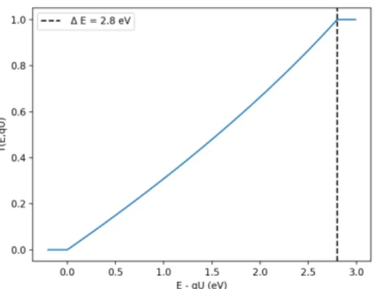
(1.5) For β scans in KATRIN with E = 18.6 keV, B _min = 0.63 mT and B _max = 4.23 T gives an energy resolution ∆ E = 2.8 eV for the main spectrometer. The transmission function of an ideal MAC-E filter at retarding potential U for an isotropic source can be written as:

T ( E, qU ) =



 

 



 

 



0 E − qU < 0

1 − r

1 −

BA

1 − r

1 −

BA

0 ≤ E − qU ≤ _∆E 1 E − qU > _∆E

(1.6)

Equation 1.6 is not valid at higher energies due to non-adiabatic effects and T ( E, qU ) < 1

for E >> qU. The ideal transmission function of a MAC-E filter with ∆E = 2.8 eV is

depicted in Figure 1.3. Assuming electron energy spectrum I ( _E ) , the integral spectrum in a MAC-E filter can be modeled as:

S ( qU ) =

Z _{+ ∞}

− _∞ I ( E ) T ( E, qU ) dE + B ( qU ) , (1.7)

with background term B ( qU ) to include all possible sources of background.

1.2. The KATRIN experiment

Figure 1.3.: Transmission function of an ideal MAC-E filter with ∆E = 2.8 eV, B _S = 4.23 T and B _A = 0.63 mT.

1.2.2. Experimental setup

Figure 1.4.: KATRIN experimental setup [13].

A schematic representation of the KATRIN experiment is shown in Figure 1.4. The setup is 70 m long and can be divided into six different sections:

a) Rear section

The rear section serves two main purposes:

• Houses the rear wall for the termination of WGTS beamtube. The rear wall is a circular disk made of stainless steel with gold-plating on the surface to create a uniform starting potential for the β electrons.

• Houses the electron gun and the Beta Induced X-ray Spectrometry (BIXS) detector.

The electron gun provides a source of mono-energetic electrons for calibration

studies and column density monitoring while the BIXS detector measures source

activity by detecting the bremsstrahlung radiation from β electrons reaching the

rear wall.

1. Introduction

b) Windowless Gaseous Tritium Source (WGTS)

The WGTS is a 10 m long and 90 mm wide beamtube made of stainless steel as shown in Figure 1.5. Molecular tritium with ≥ 95% purity is injected in the middle section of WGTS and pumped out at the ends, until a stable column density is achieved. The maximum column density in the WGTS for neutrino mass measurement is 5 · 10 ¹⁷ cm ^{− 2} . Superconducting magnets provide a homogeneous magnetic field of 2.52 T to guide β electrons toward the spectrometer. The WGTS is surrounded by a complex cryostat system to achieve temperature stability of ± 30 mK and column density stability of 0.1%.

Figure 1.5.: Cross sectional view of WGTS [15].

c) Transport section

The Transport section is divided into the Differential Pumping Section (DPS) and the Cryogenic Pumping Section (CPS). The DPS consists of five 1 m long tubes with two sections tilted at 20° to prevent direct line of sight for tritium molecules. The tritium flow is reduced by a factor of 10 ⁵ with the help of four turbomolecular pumps placed between the sections. The remaining tritium is removed in the CPS, where it is absorbed on gold plated beamtube cooled by argon frost reducing the flow further by a factor of 10 ⁷ . This drastic reduction minimizes the background from tritium present in the main spectrometer.

d) Pre-spectrometer

Most β electrons produced in the WGTS don’t carry information about the neutrino

mass but will contribute to the background in the main spectrometer. To reduce the

number of trapped electron in the main spectrometer, a smaller spectrometer made of

stainless steel, with a diameter of 1.7 m and length of 3.4 m has been placed between

the transport section and the main spectrometer. Electrons can only pass through the

pre-spectrometer if they have energy higher than 18.3 keV.

1.2. The KATRIN experiment

e) Main Spectrometer (MS)

The MS is also made of stainless steel with an inner diameter of 9.8 m and length of 23.28 m. The large diameter is necessary to conserve the magnetic flux in the analyzing plane. The MS is kept in ultra high vacuum (UHV) of 10 ^{− 11} mbar to reduce background created in the large volume of the spectrometer. A two layer electrode system is used with the inner electrodes providing the high voltage in MS while the outer electrodes keep the vessel at a relatively positive potential to the inner electrode for suppressing secondary electrons from the wall.

f) Detector section

A silicon PIN diode array of 9 cm diameter sits at the end of the flux tube. The detector is segmented into 148 equal area pixels as shown in Figure 1.6. The pixels can be analyzed individually to account for possible radial and azimuthal inhomogeneities of the electric and magnetic fields. The β electrons can also be post-accelerated to higher energies before reaching detector in order to mitigate background.

Figure 1.6.: Segmented detector of MS [9].

Monitor Spectrometer (MoS)

The MoS is an additional MAC-E filter operated in KATRIN to monitor the stability of high voltage applied in the MS during neutrino mass measurement. The monitoring is achieved by electrically coupling the MoS to the MS high voltage and measuring the energy of a conversion electron line of ^83m Kr in parallel to neutrino mass measurement.

The experimental setup at the MoS is described in chapter 3.

1. Introduction

1.2.3. Response function

Given the amount of tritium in the WGTS, the β electrons can also scatter on tritium molecules before leaving the WGTS. If the scattering is inelastic, the electron energy is changed and the transmission function must be modified to take this into account.

The probability of an electron to inelastically scatter n times at position z inside the WGTS is given by [16]:

P _n ( z ) = ¹ 1 − cos ( θ _max )

Z _θ

θ = 0 sin ( θ )

Z ₁

0 P _inel,n ( z, θ ) dθ, (1.8) with P _inel,n being the inelastic scattering probability. P _inel,n is approximated with a Poisson distribution as:

P _inel,n = ( N _eff ( z, θ ) · σ _inel ) ⁿ

n! · exp (− N _eff ( z, θ ) · σ _inel ) ,

where σ _inel is the inelastic cross section and N _{e f f} is the effective column density that electrons see while traveling through WGTS.

N _eff ( z, θ ) = ¹ cos ( θ ) ^·

Z _L/2

z ρ ( z ⁰ ) dz ⁰

The energy loss suffered by an electron in one scattering is given by : f ( e ) =







A ₁ · exp (− ₂ ( ^{e − e}

ω

2 )) e < e _c A 2 · ^ω

ω

+ 4 ( e − e

)

e ≥ e c

(1.9) The energy loss function for one scattering is shown in Figure 1.7. The energy lost in the n ^th scattering is given by convolving f ( e ) with itself ( n − 1 ) times. The convolution of the transmission function with the energy loss function is called the response function:

R ( E, qU ) =

Z _{E − qU}

0 T ( E − e, qU )

∑ ∞ i = 0

P _i · f _i ( e ) de (1.10)

1.3. Energy scale of KATRIN

Figure 1.7.: Energy loss for multiple scatterings in the WGTS.

1.3. Energy scale of KATRIN

A single measurement of the tritium β spectrum in KATRIN is taken by varying the retarding voltage applied in the MS and recording the number of electrons that reach the detector at each step. Precise knowledge of the electron energy is central to the measurement principle and unrecognized distortions of the energy scale can reduce the sensitivity to neutrino mass. The high voltage stability should be better than 3 ppm over one measurement campaign in order to reach the final neutrino mass sensitivity goal [8].

The actual potential difference seen by β decay electrons in Equation 1.6, with applied voltages V _MS at the MS and V _S at the WGTS using rear wall can be written as:

qU = ( qV _MS + φ _MS ) − ( qV _S + φ _S ) , (1.11) where q is the electric charge and φ _MS , φ _S are work function of the spectrometer and source respectively. The monitoring and calibration of the different components of the energy scale can be done by measurement of ^83m Kr conversion electrons. This thesis will focus on two particular aspects:

Main spectrometer potential

V _MS is set to about 18.6 kV in the β scans. This voltage can be measured with ppm accuracy using commercial voltmeter after scaling down to 20 V range using the K- 35 [17] and K-65 [18] voltage dividers developed for the KATRIN experiment. The stability of the voltage divider is independently monitored using measurements of ^83m Kr at the MoS and results of this measurement are summarized in chapter 3.

Source potential

The source potential V _S is provided by the rear wall and is set in the range of only a

few volts. While the applied voltage is easily measurable, the actual source potential

1. Introduction

seen by electrons is modified due to the existence of a cold low density plasma in the

WGTS. The effect of this plasma on the source potential can be estimated by dedicated

measurements of ^83m Kr at the MS as described in chapter 4.

2. ^83m Kr as a calibration tool in KATRIN

An energy scale calibration in the KATRIN experiment can be achieved by using conversion electrons of ^83m Kr [19]. The meta-stable isotope of Kr has a half-life of 1.83 h and decays through two subsequent electromagnetic de-excitation with an energy of 32.2 keV and 9.4 keV respectively. The short half-life of ^83m Kr ensures there is no long term contamination of the experimental apparatus. With an internal conversion coefficient of 2035 and 17 respectively, both decays happen primarily via the internal conversion producing electrons instead of gamma emissions.

83m Kr can be produced from electron capture decay of ⁸³ Rb. The decaying Kr atom is left in the ^83m Kr state with 74.8% probability. The half-life of this decay is 86.2 d, making it an ideal source for generating ^83m Kr for long term monitoring required in KATRIN.

83 37 Rb + e ⁻ → ^83m ₃₆ Kr + ν _e (2.1) For KATRIN, the ^83m Kr source can be produced in three different states based on the measurement goals:

• Gaseous Krypton Source (GKrS) : Gaseous ^83m Kr is introduced in the WGTS and the Kr atoms are in a very similar environment to molecular tritium in β scans.

Ideal for characterizing effects and inhomogeneities in the WGTS source potential.

• Solid Krypton Source (SKrS) : The source is produced by implantation of ⁸³ Rb into a Highly Oriented Pyrolitic Graphite (HOPG) substrate. The source is easy to manage and ideal for long term monitoring at the MoS.

• Condensed Krypton Source (CKrS) : A condensed krypton source is situated in the CPS section for energy calibration measurements in the KATRIN beamline.

Figure 2.1 shows the relative intensity of conversion electrons produced from ^83m Kr

at different energies relevant to KATRIN. The K-32 line has energy of 17.8 keV and

natural line width of 2.7 eV. Due to comparable energy to tritium endpoint, the K-32

line can be used for monitoring the Main Spectrometer HV at the Monitor Spectrometer

using the SKrS. The details of this measurement are explained in chapter 3. Further,

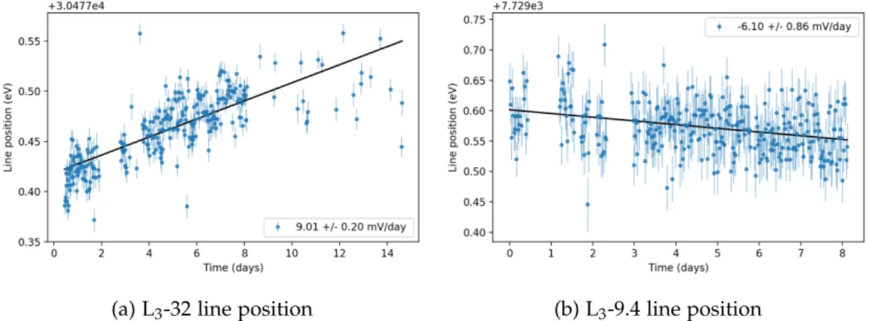
measurements of the L ₃ -32 line with energy of 30.47 keV and the N _2,3 -32 doublet at

32.14 keV will be used to estimate the space charging in the WGTS beamtube using the

GKrS. The analysis of L ₃ -32 line from this measurement is described in chapter 4.

2. ^83m Kr as a calibration tool in KATRIN

Figure 2.1.: Different mono-energetic lines of ^83m Kr [20].

2.1. Modeling of ^83m Kr conversion electron spectrum

The differential line shape of conversion electrons is a function of energy given by a Lorentzian profile:

L ( E; A, E ₀ , Γ ) = ^A π

Γ/2

( E − E ₀ ) ² + Γ ² /4 , (2.2) where Γ is the full width at half maximum (FWHM), E ₀ is line position and A is the normalization factor,

Z _{+ ∞}

− _∞ L ( E; A, E 0 , Γ ) dE = A

The line shape has an intrinsic width (Γ) due to finite lifetime of the created vacancy.

The integral spectrum for conversion electrons can then be written as S ( qU; A, E ₀ , Γ, B ) =

Z + _∞

− _∞ L ( E; A, E ₀ , Γ ) R ( E, qU ) dE + B ( qU ) , (2.3) where R is the response function and B is the background. An example integral line shape is shown in Figure 2.2.

2.2. Additional effects

While Equation 2.2 describes an ideal conversion line, few effects can modify the energy of the conversion electrons. These effects lead to additional broadening of the conversion line shape. The Lorentzian line shape is convolved with a Gaussian function G ( E; σ ) to account for the broadening. The resulting distribution is called a Voigt profile.

V ( E; A, E ₀ , Γ, σ ) =

Z _{+ ∞}

− _∞ L ( E; A, E ₀ , Γ ) G ( E − y; σ ) dy (2.4)

2.2. Additional effects

Figure 2.2.: Example differential and integral line shape for L ₃ -32 conversion electrons peak with A = 50 cps, E 0 = 30477.3 eV, B = 10 cps and MAC-E filter with B _s = 2.5 T, B _min = 2.7 · 10 ^{− 4} T and B _max = 4.2 T [21].

2.2.1. Doppler effect

For the GKrS, the decaying Kr atom has thermal motion described by the Maxwell- Boltzmann distribution. This motion also broadens the conversion electron line shape, and the broadening can be approximated by a Gaussian function of width σ dependent on the gas temperature T.

G ( E; σ ) = √ ¹ 2πσ ² e

2

2σ2

(2.5)

with

σ =

r 2Ek B Tm

M ,

where m is the mass of electron, k _B is the Boltzmann constant and M is mass of krypton atom.

2.2.2. Synchrotron loss

Energy loss due to emission of synchrotron radiation happens when electrons are traveling in a gyrational motion in magnetic fields. The energy loss can be calculated as:

∆ E = − ^{q 4}

3πc ³ e 0 m ³ _e E _⊥ γ + 1

2 B ² t, (2.6)

where E ⊥ is the transversal electron energy, t is the time spent by electron in the magnetic

field B and γ is the relativistic correction factor. As the energy loss is proportional to B ² ,

the synchrotron loss primarily happens in the WGTS and the front transport system in

KATRIN.

2. ^83m Kr as a calibration tool in KATRIN

2.3. Parameter Inference from data

The measured spectrum is fit to the theoretical prediction described above. The analysis is done using the maximum likelihood estimator. The estimator can be used to find the best set of parameters θ in a given model S(θ), after making N _obs observations. For n independent measurements in a single spectrum, the likelihood function of θ is given as:

L ( θ ) = P ( N _obs | θ )

=

∏ n i = 1

p ( N _obs,i | θ ) ^(2.7)

with p ( N _obs,i | θ ) being the probability of observing N _obs,i counts under the assumption of model parameters θ. Then, the optimal set of parameters can be obtained by maximizing the likelihood function (or minimizing the negative log likelihood function which is numerically easier). The probability of observed counts N _obs,i from a decay follows Poisson distribution. But for large values of N, the probability can be approximated with a Gaussian distribution as well:

p ( N _obs,i | θ ) = _q ¹ 2πσ _i ²

e ⁻

(_Nobs,i−S(_θ))² 2σ2

i

, (2.8)

and the negative log likelihood is given as (dropping the constant term):

− ln L ( θ ) = ¹ 2

∑ n i = 1

( N _obs,i − S _i ( θ )) ² σ _i ²

= ¹ 2 χ ² ( θ )

(2.9)

Thus, the best set of parameters can be found by minimizing the chi-square function (χ ² ). Assuming an underlying multivariate normal distribution, the uncertainties on the best fit can be determined for n standard deviations by finding the value of parameters θ that satisfies:

χ ² ( θ ) − χ ² _min = n ² (2.10)

3. Monitoring the main spectrometer high voltage

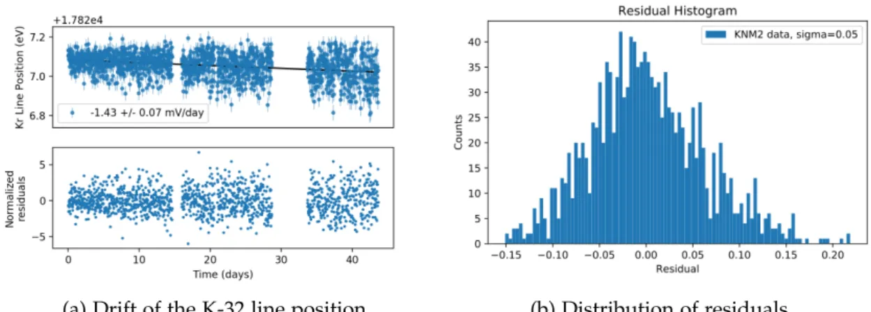
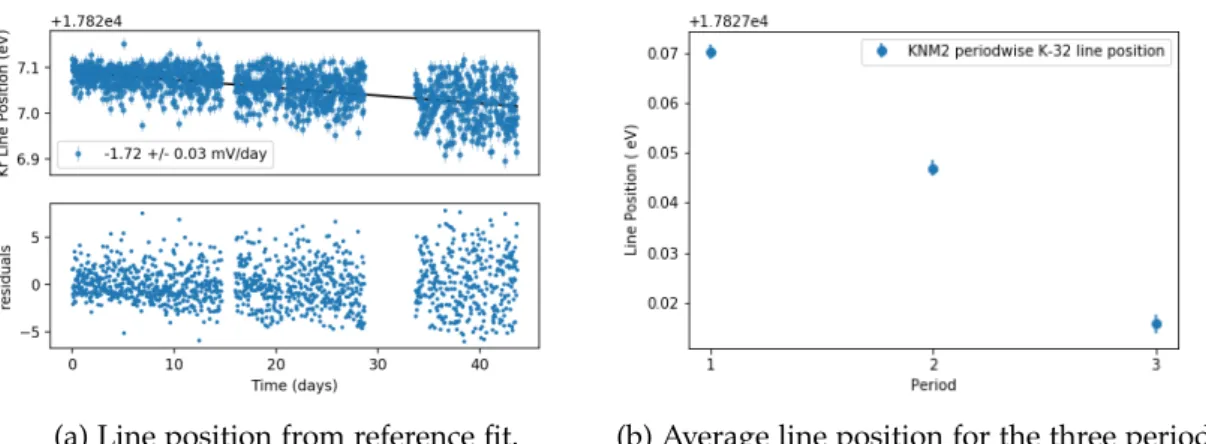
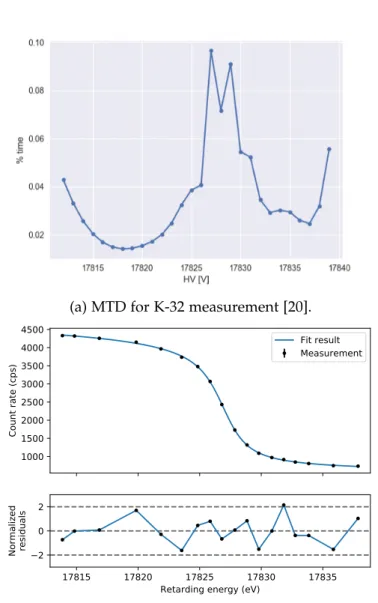
The spectrometer used in the Mainz neutrino mass experiment has been refurbished in KATRIN as the monitor spectrometer (MoS). The main goal of the MoS operation is to assess the long-term stability of the main spectrometer high voltage (MS HV) in parallel of the neutrino mass measurement. To do so, the K-32 line of ^83m Kr is scanned at the MoS while being electrically coupled to the MS HV. The line position of the K-32 line provides an independent assessment of the MS HV stability during the β scans in the neutrino mass measurement.

3.1. Motivation

Commercial high precision voltmeter can be used to measure voltages with ppm accuracy but only in the 20 V range while the voltage applied at the MS is set to 18.6 kV in the tritium β scans. To scale down the voltage from 18 kV to 20 V, very precise voltage dividers named K-35 (and K-65) have been developed in KATRIN. Once the voltage has been scaled down using the divider, a Fluke 8508A voltmeter is used to measure the voltage with ppm precision.

The voltage divider is calibrated before every neutrino mass measurement campaign but the stability of the divider must be monitored during the actual measurement as well to ensure the . This monitoring is achieved by coupling the MoS retarding electrode to the MS HV and performing regular measurements of ^83m Kr conversion electrons in the MoS.

For this measurement, the K-32 line of ^83m Kr has an important advantage. Since the energy of K-32 conversion electron (17.8 keV) is close to the tritium endpoint (18.6 keV), it is possible to scan the K-32 line at MoS in parallel to β scans in the MS. This provides an unique opportunity to monitor the stability of the voltage divider while in operation, an important cross-check for HV stability in KATRIN.

3.2. Experimental setup of MoS

Spectrometer vessel

A drawing of the MoS setup is shown in Figure 3.1. The spectrometer vessel is made of

stainless steel with a length of 3 m and diameter of 1 m. The vessel itself is grounded and

a set of solid filter electrodes is used to apply retarding potential inside the vessel. The

vessel is kept in ultra-high vacuum (UHV) of 10 ^{− 10} mbar with the help of turbomolecular

3. Monitoring the main spectrometer high voltage

pumps to reduce inelastic scattering of the electrons on residual gas in the vessel.

Superconducting coils generate magnetic field B _max of 6 T at the boundaries while the magnetic field in the analyzing plane B _min is set by the low field correction system (LFCS) at 0.35 mT. Another set of coils called the Earth magnetic compensation system (EMCS) correct for the Earth magnetic field inside the spectrometer vessel. Using Equation 1.5, the energy resolution of MoS at the K-32 line energy (17.8 keV) is 1.04 eV.

Figure 3.1.: CAD drawing of MoS setup [20].

Source

The source for MoS is produced by implantation of ⁸³ Rb into a Highly Oriented Pyrolitic Graphite (HOPG) solid substrate. The holding structure is made of ceramic disk with four independent slots for mounting different sources as shown in Figure 3.2. The base flange of the chamber is mounted in a cross table to allow axial movement. It is possible to switch between the different sources without breaking the source chamber vacuum.

Figure 3.2.: Source holder of MoS [22].

Detector

The detector consists of a single circular silicon PIN-diode (Canberra PD-150-12-500AM)

surrounded by four auxiliary windowless PIN-photo diodes (Hamamatsu S3590-09) as

shown in Figure 3.3a. The auxiliary pixels are used for aligning the central detector with

3.2. Experimental setup of MoS

the source. The deadtime of the detector is estimated by injecting a pulser of frequency 200 Hz in the detector. If N _e is the measured electron count, and N _p is the pulser count, the true electron count can be calculated as

N = ^{f · t}

N _p N _e , (3.1)

with t being the measurement time. An example ADC histogram of the K-32 line taken using the detector is shown in Figure 3.3b.

(a) Photo of the detector [23]

DetectorAdc

Entries 43564 Mean 93.26 Std Dev 19.05

0 50 100 150 200 250

ADC 0

200 400 600 800 1000 1200 1400 1600 1800

2000

DetectorAdc

Entries 43564 Mean 93.26 Std Dev 19.05

mos00192025.1

(b) Example histogram from one measurement Figure 3.3.: Detector of the MoS.

High voltage

For the SKrS, the analyzing voltage V _ana does not depend on the source work function φ _source , since the Kr atom is sitting inside the solid substrate environment. V _ana can be then written as:

qV _ana = qV _vessel + φ _vessel − qV _source , (3.2)

where V _vessel is the potential in the MoS vessel set by the retarding electrodes, V _source is the potential at the MoS source and φ _vessel is the work function of the MoS vessel. The source voltage can be set in the range of 0 − 1 kV and measured using a Fluke 8508A voltmeter after scaling down by a commercial voltage divider (Fluke 752A). For setting the vessel voltage, there are two options available:

• stand-alone mode: MoS vessel voltage is provided by a local power supply (up to 35 kV). The voltage is measured by a Fluke 8508A voltmeter after scaling down using a commercial JRL divider ¹ . This mode is useful for MoS operation independent to neutrino mass measurements at MS.

1 Julie Research Laboratories, model KV-50

3. Monitoring the main spectrometer high voltage

• coupled mode: MoS vessel is electrically coupled to the MS HV ( 18.6 kV in β scans) for monitoring the stability. The vessel voltage is independently measured by the JRL divider as well.

3.3. Possible sources of drift in MoS

A possible drift in the K-32 line position can either be due to the K-35 divider or due to different systematics related to the MoS. Identifying the source of drift is crucial for meaningful assessment of HV stability in the MS. Following sources of drift can be expected in the MoS setup:

Source drift

The SKrS can have inherent drift in the energy of conversion electron due to changing substrate environment over time. The line position stability for the possible choices was studied and the HOPG-substrate based source were found to be stable at sub-ppm level [20]. For the new batch of sources used at the MoS, the measurement of L 3 -lines and measurements with two different HOPG sources can be used to examine the source stability.

Time synchronization drift

If there are time synchronization issues in the data acquisition from slow control param- eters like the voltmeter readings, the net effect on line position adds over continuous measurements. The effect can be identified by scanning the K-32 line consecutively in up and down direction. Scanning in the up direction means the spectrum is measured by monotonically increasing the analyzing voltage and vice versa.

MoS work function drift

The work function of the retarding electrode in the MoS vessel can change due to adsorption of residual gases in the MoS vessel. As the actual retarding voltage seen by the conversion electrons will change according to Equation 3.2, even if the externally applied voltage at source and vessel are same, the K-32 line position will also drift.

Voltage divider drift

For a voltage divider with dividing ratio M, the output voltage U _out is related to the input voltage U as:

U = MU out (3.3)

Assuming the voltage divider is drifting and the dividing ratio is changed to M’ in a

later measurement. The measured electron energy in the first measurement would be

3.4. Krypton measurements at MoS

qU = qMU out and in the second measurement qU ⁰ = qMU _out ⁰ , with qU = qM ⁰ U _out ⁰ if the actual electron energy is constant. The difference in observed line position would be:

q ( U ⁰ − U ) = q ( MU _out ⁰ − U )

∆ qU = qU ( ^M

M ⁰ − 1 ) ^(3.4)

Thus, the observed drift ∆ qU is dependent on the energy scale (U) of the measured line.

In contrast, a drift of the spectrometer work function (ϕ) will be independent of energy scale according to Equation 3.2. Thus, measurements of two different energy scales can be used to distinguish between a voltage divider drift and a MoS systematic drift.

3.4. Krypton measurements at MoS

Line shape

The Voigt line shape was found to be insufficient for explaining the observed conversion electrons line at MoS due to asymmetry at lower energies [22]. The Doniach-Sunjic line shape ( f _DS ) was identified as a suitable choice in [24] with parameter α to account for the observed asymmetry. For α = 0, the line shape is equivalent to a Lorentzian line shape. To account for the broadening, f _DS is convolved with a Gaussian to give the final line shape ( f _DSG ),

f _DS ( E; a, E _i , Γ _i , α ) = ^a

π [( E − E _i ) ² + Γ _i ² /4 ]

^cos πα

2 + ( 1 − α ) arctan

E − E _i Γ _i /2

f _DSG ( E; a, E _i , σ, Γ _i , α ) =

Z + _∞

− _∞ G ( E − y; σ ) f _DS ( y; a, Ei, Γ _i , α ) dy,

(3.5)

where a is the amplitude (normalization factor), E _i is the line position, σ is the Gaussian broadening of line width and Γ _i is the intrinsic line width.

K-32 line

A single measurement of the spectrum is called a run and consists of measuring the number of electrons at retarding voltages around the line position. The retarding voltages and the time spent at each step are defined by the measuring time distribution (MTD).

For K-32 line, the MTD used for scanning the K-32 line is shown in Figure 3.4a. A single

run with enough statistics for measuring stability at ppm level requires approximately

500 s given the activity of the available source (with additional 3 s waiting time for

switching voltage at each step). In coupled mode, the vessel voltage is kept constant for

the full duration and scanning is achieved by varying the source voltage. On average,

three K-32 scans are performed at the MoS for each β scan in the MS. An example K-32

spectrum fitted using the χ ² -minimization is shown in Figure 3.4b.

3. Monitoring the main spectrometer high voltage

L ₃ lines

Measurements of L ₃ lines can be used to explore the line position stability in MoS at another energy scale apart from the K-32 line. This measurement is an important input for differentiating between an energy dependent drift due to the K-35 divider and a constant drift due to other MoS systematic effects. Further, the L ₃ -9.4 (7.73 kV) and L ₃ -32 (30.48 kV) line come from the same atomic shell and thus experience similar atomic affects in the source. Thus, the comparison of L-lines is useful for absolute scale calibration of the MoS setup.

(a) MTD for K-32 measurement [20].

1000 1500 2000 2500 3000 3500 4000 4500

Count rate (cps)

Fit result Measurement

17815 17820 17825 17830 17835

Retarding energy (eV) 2

0 2 Normalized residuals

(b) Fitted K-32 line using the Doniach-Sunjic line shape.

Figure 3.4.: Measurement of K-32 line of ^83m Kr at MoS.

3.5. Measurement campaigns

3.5. Measurement campaigns

The data analyzed in this thesis include measurements:

• in the coupled mode for monitoring the stability of MS HV in the second and fourth neutrino mass measurement campaign (KNM-2 and KNM-4).

• for understanding the MoS systematic effects in the stand-alone mode during the third neutrino mass measurement campaign (KNM-3).

3.5.1. KNM-2

The MoS was coupled to the MS HV and continuous K-32 scans were performed for approximately 44 days between 1 ^st of Oct. 2019 and 14 ^th of Nov. 2019. The source used for this measurement is denoted as HOPG-8-8 and the surface activity of this source is shown in Figure 3.5. The source activity from this measurement was determined to be 1.9 MBq. A total of 1412 runs were fitted in the KNM-2 measurement and the

0 50 100 150 200 250

0 50 100 150 200 250

0 500 1000 1500 2000 2500 3000 3500 4000 4500 5000

HOPG-8-8, 17.07.2019

Figure 3.5.: Surface activity of HOPG-8-8 [25].

distribution of the reduced χ ² is shown in Figure 3.6. A few runs show exceptionally high reduced χ ² and an upper limit of 5 was chosen to remove the outliers. Further, some runs also suffered from numerical stability issue in the fitting procedure and had to be removed since the parameter estimation was not reliable. The total number of runs removed was 49, giving a selection efficiency of 93.4%.

The fitted line position of the K-32 spectrum is shown in Figure 3.7a and the distribution

of line position with the reduced χ ² is shown in Figure 3.7b and it can be observed that

3. Monitoring the main spectrometer high voltage

Figure 3.6.: Reduced χ ² of K-32 runs in KNM-2.

the line position does not show strong dependence on the fit quality. Evolution of the other 4 fitted parameters and some important parameter correlations are also plotted in Figure A.1 and Figure A.2. The fitted line position shows good stability considering

(a) Line position evolution over time (b) Distribution of line position vs reduced χ ²

Figure 3.7.: K-32 line position from KNM-2 measurement.

the long measurement duration. The fluctuations of line position show an increase over time, which can be attributed to lower activity of the source. A linear drift of

− 1.43 ± 0.07 mV/day can be fitted to the line position as shown in Figure 3.8a. The

drift translates to line position stability of 3.5 ppm over KNM-2, proving that the MoS is

capable of measuring MS HV stability at ppm level. The distribution of residuals from

the linear fit can be approximated with a Gaussian distribution with variance of 0.05

eV as shown in Figure 3.8b. The statistical error bar on the line position from a single

3.5. Measurement campaigns

fit is 0.03 eV, which means that there are unaccounted systematic effect broadening the observed distribution.

(a) Drift of the K-32 line position. (b) Distribution of residuals.

Figure 3.8.: Fitting linear drift in K-32 line position from KNM-2 measurement.

Rate estimation

The count rate of electrons in a subrun is estimated by integrating the ADC histogram.

The integration boundary is manually fixed to 50-120 and the effect of changing the integration boundaries on the line position drift was studied. A maximum variation of 0.05 mV/day was observed in the line position drift for the KNM-2 data for different integration boundaries. Thus, the observed deviation is found to be negligible compared to the observed drift.

Consistency check

The K-32 data was also reanalyzed using the following two methods:

• Reference method:

Ideally, the shape of the spectrum is not expected to change drastically between measurements with the same source. Fixing the shape (σ and α) to a reference spectrum reduces the fit to only three free parameters and thus give smaller uncertainty on line position. With σ _avg = 0.48 eV and α _avg = 0.05 as input ² , drift of − 1.72 ± 0.03 mV/day is observed from the reference fit shown in Figure 3.9a.

• Period wise averaged data:

Multiple consecutive measurements is stacked together before fitting to reduce the error on fitted line position. Difference of 54.28 mV is observed between the average line position in the first and third period as shown in Figure 3.9b, in agreement with the earlier observed drift.

2 average values of the 5 parameter fit

3. Monitoring the main spectrometer high voltage

(a) Line position from reference fit. (b) Average line position for the three periods.

Figure 3.9.: K-32 line position from reference fit and periodwise fit in KNM-2.

Comparison with JRL divider

Since the vessel voltage is also independently measured using the JRL divider, the K-32 measurements can also be analyzed using the JRL readings. First four days of measurements were excluded from the comparison because the JRL divider is expected to take some days for voltage stability at the required precision. The line position fitted with JRL data is compared to the K-35 results by analyzing runs available in both datasets as sown in Figure 3.10a. A constant shift of > 1 eV can be seen in the line position from K-35 vs JRL divider due to known calibration difference. The strong correlation between the line position from two dividers clearly indicates that the MoS setup should be the primary cause of the observed line position drift. The profile likelihood scan of relative drift between the two dividers is also shown in Figure 3.10b, giving 1σ upper limit of 0.22 mV/day (0.5 ppm over KNM-2) on the relative drift between the two dividers.

(a) K-32 line position. (b) Profile likelihood for a relative drift.

Figure 3.10.: K-32 runs analyzed using K-35 and JRL voltage dividers.

3.5. Measurement campaigns

L ₃ measurements in KNM-2

While there were few measurements of L 3 lines in KNM-2, the data was not useful for the following reasons:

• L ₃ measurements were only done on the 1 ^st of Oct. 2019 and 22 ^nd of Oct. 2019.

Measurements at only two time points are not enough for estimating stability at the required precision.

• L ₃ -9.4 suffered from low count rate and high background noise. An example spectrum is shown in Figure 3.11

• L 3 -32 measurements were not reliable as the source voltmeter was disconnected and no voltmeter readings were recorded for the first L ₃ -32 measurement.

Figure 3.11.: Fitted L ₃ -9.4 spectrum in KNM-2

The result from analysis of MoS operation in KNM-2 were summarized for the col- laboration in [26]. The following recommendations were identified for the future measurements:

• Scans should be done in consecutive up and down direction to identify if there is a time synchronization effect.

• Two ⁸³ Rb source should be used in the same measurement campaign to understand source effects on the line stability.

• Regular L ₃ measurements with high statistics are necessary for better understand- ing of the observed drift.

3.5.2. KNM-3

A new source (HOPG-8-9) was installed in the MoS on 10 ^th of Mar. 2020 with activity of

3.79 MBq. Further, the data acquisition system of MoS was upgraded to ensure proper

3. Monitoring the main spectrometer high voltage

time synchronization between the different MoS components. The measurements in the stand-alone mode started on 20 ^th of May. 2020 and lasted until 08 ^th of Sept. 2020. The same MTD (Figure 3.4a) was used for L 3 measurement but with 0.5 V steps around the L ₃ line position due to the sharper line width. The goal of these measurements was to understand the effect of different MoS components on the line position.

Effect of various MoS systematics on observed drift

The evolution of line position in different settings for the K-32 line is shown in Fig- ure 3.12 and for the L ₃ lines in Figure 3.13. Further, the observed line position drift are summarized in Table 3.1.

Table 3.1.: MoS measurement in KNM-3 using JRL voltmeter in stand-alone mode

Line V _source range Time (days) Drift (mV/day)

HOPG-8-9 (new source)

K-32 750 V 10 − 1.32 ± 0.17

50 V 5 − 15.79 ± 0.52

L ₃ -32 750 V 10 9.01 ± 0.20

L 3 -9.4 750 V 8 − 6.10 ± 0.86

HOPG-8-8 (old source)

K-32 50 V 5 − 2.86 ± 2.16

The following observations can be made:

• Measurements were performed in consecutive up and down scans and no time synchronization issue were found.

• Measurements with source voltmeter at 750 V and 50 V show that the drift is independent of the source voltmeter scale.

• Measurement using HOPG-8-9 and HOPG-8-8 show that the drift is not originating from the source.

• Measurements for L ₃ -32 and L ₃ -9.4 drift in opposite directions.

The L 3 line position behavior is not expected from the sources of drift identified in sec-

tion 3.3. New systematic measurements at MoS would be necessary to understand

the L ₃ measurements. Further, a detailed review of L ₃ measurement is also required

to understand whether there is some unaccounted physical effect in the L 3 analysis

introducing the observed deviation.

3.5. Measurement campaigns

(a) HOPG-8-9 source, V source at 750 V (b) HOPG-8-9 source, V source at 50 V

(c) HOPG-8-8 source, V source at 50 V

Figure 3.12.: Line position from K-32 measurement in KNM-3.

(a) L 3 -32 line position (b) L 3 -9.4 line position

Figure 3.13.: L ₃ -32 measurement in KNM-3 with HOPG-8-9 source, V _source at 750 V.

3. Monitoring the main spectrometer high voltage

3.5.3. KNM-4

The MoS was coupled to the MS again and the K-32 line was continuously measured using the HOPG-8-9 source from 11 ^th of Sept. 2020 until 21 ^st of Oct. 2020. Due to temperature stabilization issue in the K-35 voltage divider, it was switched with the K-65 divider in the MS on 22 ^nd of Sept. 2020. The fitted line position for the data with the standard 5 parameter fit is shown in Figure 3.14. The overall drift is fitted for two different scenarios:

• A common slope in the data with an additional offset due to K-35/K-65 switch (red line).

• A common slope in the data but no offset (black line).

(a) Line position evolution (b) Histogram of line position

Figure 3.14.: K-32 measurements in KNM-4.

Using the average values of σ _avg = 0.464 eV and α _avg = 0.089, the data was refitted using the reference method and the result is shown in Figure 3.15.

(a) Line position evolution (b) Histogram of line position

Figure 3.15.: Reference fit of K-32 measurement in KNM-4.

3.6. Long term evolution of K-32 line position

From the K-32 data in KNM-4, one can see that:

• The MS HV shows stability of 0.15 ppm over 38 days of measurement from the reference fit.

• Both voltage dividers are in very good agreement and do not introduce a HV fluctuation in β scans due to switching.

3.6. Long term evolution of K-32 line position

The K-32 line position measured from KNM-2 to KNM-4 is shown in Figure 3.16. The line position in KNM-3 is higher by approx. 1.1 eV as the data was analyzed using the JRL divider. The line position shows a reset after continuous measurements are stopped.

This behavior clearly excludes the voltage divider used in MS as the source of drift. The most likely explanation for such a behavior would be a work function drift of the MoS vessel. Further, from the combination of measurement in the coupled mode in KNM-2 and KNM-4, a drift of 0.14 ± 0.003 mV/day can be fitted to the data. The drift translates to 3 ppm stability over a long duration of 380 days, confirming that the MS HV meets the stability requirement during the β scans.

Figure 3.16.: Line position of K-32 line from MoS measurements.

3. Monitoring the main spectrometer high voltage

3.7. Conclusion

The MS HV stability is an important systematic component of KATRIN with a strict requirement of ≤ 3ppm variation over one measurement campaign lasting 2 months.

The MS HV stability is essentially dependent on the voltage divider used for diving the voltage down from 18.6 keV to 20 V before it can be measured with precise voltmeters.

The MoS was coupled to the MS HV and continuous measurement of K-32 line of ^83m Kr were taken to assess the HV stability in parallel to β scans in the MS. Following drifts were seen in the K-32 line position in the coupled mode:

• 3.5 ppm over 44 days in KNM-2 reduced to 0.5 ppm when compared with JRL divider.

• 0.15 ppm over 38 days in KNM-4.

• 3 ppm over 380 days combining the KNM-2 and KNM-4 measurement.

Further, systematic measurements of K-32 and L ₃ lines were performed at the MoS in the stand alone mode to understand the origin of the small drift observed. The analysis of these measurements is useful in excluding the following systematic sources of drift:

• Time synchronization.

• ⁸³ Rb source.

• Source voltmeter energy scale.

The K-32 line position in the coupled mode shows much better stability in KNM-4 compared to KNM-2. This observation could be explained by possible time synchro- nization issue in KNM-2 measurements as the MoS DAQ was only updated afterwards.

The agreement in the combined dataset also provides additional evidence of long term

stability of the MS HV as well as the MoS components. Yet, the analysis of L 3 line in

the stand alone mode using the JRL divider shows a strong positive drift in L ₃ -32 line

but negative drift in the L ₃ -9.4 line. This behavior can not be explained by the known

sources of drift but it is important to note that the L 3 measurement is limited by short

term instabilities of the JRL divider. Thus, better systematic studies would be needed in

the future to completely understand the MoS energy scale.

4. Source potential characterization

An equally important part of the energy scale of KATRIN is the source potential in the Windowless Gaseous Tritium Source (WGTS). There can be spatial or temporal fluctuations in the source potential due to existence of a cold low density plasma, leading to broadening of the tritium spectrum. If not quantified precisely, this broadening will lead to a bias in the resulting neutrino mass. Measurements of mono-energetic lines of ^83m Kr in the main spectrometer (MS) can be used to estimate the broadening of the source potential using the Gaseous Kr Source (GKrS) in the WGTS. These measurement are also useful for understanding the evolution of plasma with different experimental parameters of KATRIN, an important input for optimizing the operation of KATRIN in future measurement campaigns.

4.1. Origin of source potential variations

The WGTS has been briefly described in section 1.2. Highly energetic electron from the β decay can ionize the neutral T ₂ molecules, creating many secondary electrons and positive ions (T ⁺ , He ⁺ , ( ³ _HeT ⁺ ) ). This process leads to formation of a cold low energy plasma in the WGTS. The source potential experienced by electrons in the WGTS thus becomes dependent on both the plasma and the boundary conditions (rearwall and the WGTS beam tube). The plasma potential can show following inhomogeneities:

• Spatial Inhomogeneity:

The gas density profile in the WGTS has a strong gradient from the center towards the outer boundary on both sides as shown in Figure 4.1. The plasma potential is expected to have spatial variations driven by the gas density profile. The inhomogeneities can be in both radial and longitudinal direction due to the large size of WGTS beamtube. The segmented detector used in KATRIN can account for the radial differences but estimating the broadening due to the longitudinal component is still necessary.

• Temporal Inhomogeneity:

Time dependent surface potential in the WGTS can be either due to changing

boundary conditions (work function of the beamtube or rearwall) or because of

plasma fluctuations. The plasma fluctuations will create time dependent electric

field inside the WGTS. If the time scale of these oscillation is similar to the time of

flight of the β electrons in the WGTS, this effect will also broaden the signal.

4. Source potential characterization

Figure 4.1.: Gas density profile at 35% column density in WGTS for tritium (blue) and krypton (orange) [27].

4.2. Krypton characterization using GKrS

Using the GKrS, ^83m Kr measurement can be performed in the MS in the following ways:

• Kr+Tr mode:

Both krypton and tritium are circulated together and thus share the same volume in the WGTS. The conversion electrons of ^83m Kr are affected by the plasma created due to β decay of tritium. Measurements in this mode can be used to estimate the effect of plasma on the source potential.

• Kr-only mode:

Only krypton is circulated in the WGTS. The measurement in Kr-only mode provides the line position and width of the conversion electrons without plasma effects. This measurement is useful for characterizing the source potential in the absence of tritium plasma.

The K-32 line of ^83m Kr is superimposed on tritium background in the Kr+Tr mode and

cannot be used for plasma measurements. The L ₃ -32 line at 30.47 keV is interesting due

to the high line intensity and sharper line width (approx. 1 eV). Further, the N 2,3 -32 line

doublet is also useful due to its negligible line width but requires higher measurement

time due to the low intensity of the doublet.