JOURNAL OF GEOPHYSICAL RESEARCH
Supporting Information for ”Variability of the Atlantic North Equatorial Undercurrent and its impact on oxygen”
K. Burmeister1, J. F. L¨ubbecke1,2, P. Brandt1,2, and O. Duteil1
1GEOMAR Helmholtz Centre for Ocean Research Kiel, D¨usternbrooker Weg 20, 24105 Kiel, Germany
2Christian-Albrechts-Universit¨at zu Kiel, Christian-Albrechts-Platz 4, 24118 Kiel, Germany
Contents of this file
1. Figures S1 to S4 Introduction
The supplementary information contains four figures (Fig. S1-S4). These figures are realized using simulation SIM1 and SIM2 of the conceptual model, ship observations along 23◦W, the MIMOC climatology (Schmidtko et al., 2017), and HadISST data (retrieved from https://climatedataguide.ucar.edu/climate-data/sst-data-hadisst-v11).
Corresponding author: Kristin Burmeister, GEOMAR Helmholtz Centre for Ocean Research Kiel, D¨usternbrooker Weg 20, 24105 Kiel, Germany (kburmeister@geomar.de)
X - 2 BURMEISTER ET AL.: NEUC VARIABILITY AND ITS IMPACT ON OXYGEN
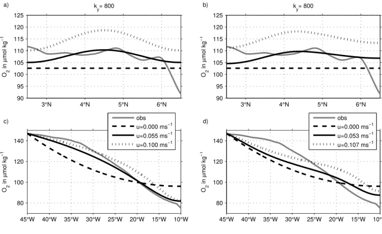
Figure S1. Black lines show (a,b) the meridional and (c,d) the zonal oxygen distribution along 23◦W and 4.5◦N, respectively, as simulated from Equ. 3 with kx = ky = 800 m2s−1 and three different u (velocity maximum) using (a,c) only the background flow field (Eq. 4, where u0 = 0 m s−1, 0.055 m s−1, and 0.1 m s−1 for the dashed, solid, and dotted line, respectively) and (b,d) superimpose a recirculation on the background flow field (Eq. 4+7, where u0 = u1 = 0 m s−1, 0.035 m s−1, and 0.14 m s−1 for the dashed, solid, and dotted line, respectively). The observations (gray lines) are oxygen concentrations along the 26.5 kg m−3 isopycnal from (a,b) the mean ship section along 23◦W and (c,d) the MIMOC climatology (Schmidtko et al., 2017).
BURMEISTER ET AL.: NEUC VARIABILITY AND ITS IMPACT ON OXYGEN X - 3
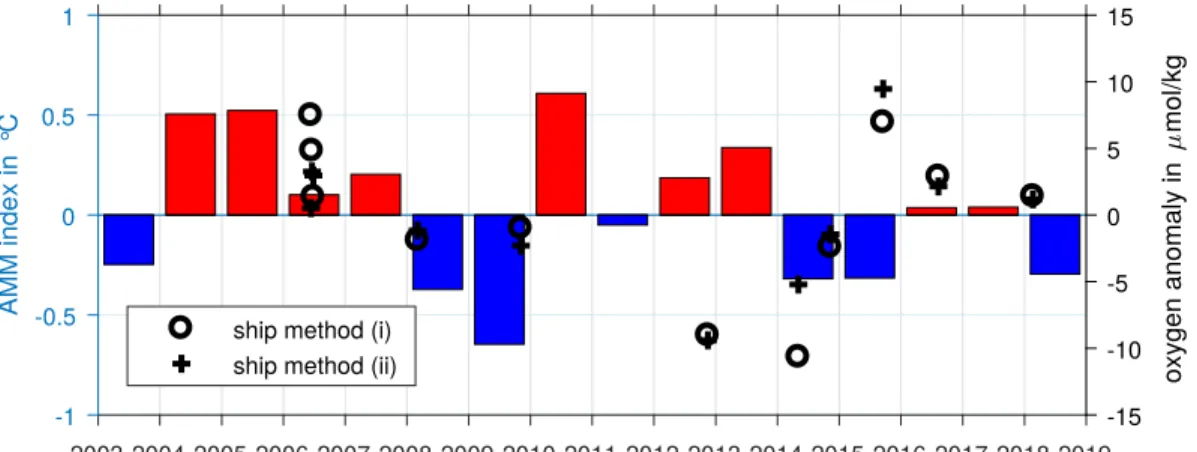
Figure S2. Left y-axis shows the monthly mean AMM index after Servain (1991) derived from HadISST data (red and blue bars, retrieved from https://climatedataguide.ucar.edu/climate- data/sst-data-hadisst-v11). Right y-axis shows oxygen anomalies derived from ship sections (total mean is substracted) averaged in NEUC region using 2 methods. (i) The values are average in a meridionally varying frame (100-300 m depth, (YCM−1.5)◦ - (YCM+ 1)◦N) (crosses).
(ii) The values are averaged in a fixed box (100-300 m depth, 3◦-6.5◦N) (circles).
X - 4 BURMEISTER ET AL.: NEUC VARIABILITY AND ITS IMPACT ON OXYGEN
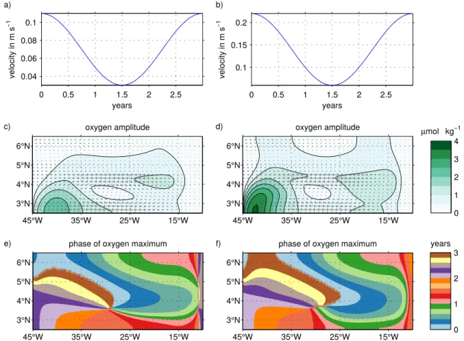
Figure S3. Amplitude of the time varying forcing (a,b), distribution of oxygen amplitude (shading in c,d) and distribution of phase of oxygen maximum (e,f) simulated by two experiments with the conceptual model (Eq. 3). Gray arrows in c-d) show the mean horizontal flow field. Both experiments study oxygen changes associated with a steady mean flow that is superimposed by a temporally varying recirculation. They are based on SIM 2. The following velocity amplitudes are used for a,c,e: the velocity amplitude of the steady mean field (Eq. 4) isu0 = 0.035 m s−1, the velocity amplitude of the time varying recirculation (Eq. 7) isu1 = 0.07 m s−1+0.04 m s−1·sin(t).
The following velocity amplitudes are used for b,d,f: the velocity amplitude of the steady mean
BURMEISTER ET AL.: NEUC VARIABILITY AND ITS IMPACT ON OXYGEN X - 5
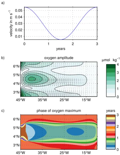
Figure S4. Amplitude of the time varying forcing (a), distribution of oxygen amplitude (shading in b) and distribution of phase of oxygen maximum (c) simulated with the conceptual model: This experiment studies oxygen changes associated with a time varying mean flow that is superimposed by a temporally constant recirculation. It is based on SIM 2. Here, a sinusoid withA= 0.025 m s−1 is superimposed onu1 of the background flow field (Eq. 7, Fig. 11b). Gray arrows in b) show the mean horizontal flow field.