Wind stress forcing of the freshwater distribution in the Arctic and North Atlantic Oceans

(1)

Wind stress forcing of the freshwater distribution in the Arctic and North Atlantic Oceans

by

Tamás Kovács

a Thesis submitted in partial fulfillment of the requirements for the degree of

Doctor of Philosophy in Geosciences

Approved Dissertation Committee

Prof. Dr. Rüdiger Gerdes

(Jacobs University Bremen; Alfred Wegener Institute)

Prof. Dr. Joachim Vogt

(Jacobs University Bremen)

Prof. Dr. Gerrit Lohmann

(Alfred Wegener Institute)

Dr. Michael Karcher

(Alfred Wegener Institute)

Dr. Benjamin Rabe

(Alfred Wegener Institute) Date of Defense: November 18, 2019

Department of Physics & Earth Sciences

(2)

(3)

iii

Statutory Declaration

Family Name, Given/First Name Kovács, Tamás

Matriculation Number 20331752

Kind of thesis submitted PhD-Thesis

English: Declaration of Authorship

I hereby declare that the thesis submitted was created and written solely by myself without any external support. Any sources, direct or indirect, are marked as such. I am aware of the fact that the contents of the thesis in digital form may be revised with regard to usage of unauthorized aid as well as whether the whole or parts of it may be identified as plagiarism. I do agree my work to be entered into a database for it to be compared with existing sources, where it will remain in order to enable further comparisons with future theses. This does not grant any rights of reproduction and usage, however.

The Thesis has been written independently and has not been submitted at any other university for the conferral of a PhD degree; neither has the thesis been previously published in full.

German: Erklärung der Autorenschaft (Urheberschaft)

Ich erkläre hiermit, dass die vorliegende Arbeit ohne fremde Hilfe ausschließlich von mir erstellt und geschrieben worden ist. Jedwede verwendeten Quellen, direkter oder indirekter Art, sind als solche kenntlich gemacht worden. Mir ist die Tatsache bewusst, dass der Inhalt der Thesis in digitaler Form geprüft werden kann im Hinblick darauf, ob es sich ganz oder in Teilen um ein Plagiat handelt. Ich bin damit einverstanden, dass meine Arbeit in einer Datenbank eingegeben werden kann, um mit bereits bestehenden Quellen verglichen zu werden und dort auch verbleibt, um mit zukünftigen Arbeiten verglichen werden zu können. Dies berechtigt jedoch nicht zur Verwendung oder Vervielfältigung.

Diese Arbeit wurde in der vorliegenden Form weder einer anderen Prüfungsbehörde vorgelegt noch wurde das Gesamtdokument bisher veröffentlicht.

...

Date, Signature

(4)

iv

(5)

v

Abstract

Observations from recent decades suggest an opposing variability between salinity anomalies in the Arctic Ocean and in the Subarctic North Atlantic, often expressed as changes in their freshwater budgets. However, due to the still too short time periods covered by observations, the temporal robustness of this covariability remains an open question. Moreover, certain patterns of freshwater variability have been linked to different atmospheric circulation regimes, but the drivers of freshwater redistribution between the two basins are still not completely understood.

The hypothesis of this study was that there is a potential for an oscillating covariability between the freshwater content of the Arctic Ocean and the Subarctic North Atlantic, and the redistribution between their basins is governed by wind stress forcing associated with large-scale patterns of atmospheric variability. In order to test this hypothesis, numerical model simulations were performed with different coupling configurations of the Max Planck Institute Earth System Model (MPI-ESM) with the objectives to 1) analyze the link between Arctic and Subarctic North Atlantic freshwater anomalies, to 2) identify key patterns of atmospheric variability that govern these anomalies through wind forcing, and to 3) explain the physical mechanisms of coupling between freshwater and near-surface winds associated with these key patterns.

The results showed that even though there is a stable sign of freshwater redistribution between the Arctic and the Subarctic North Atlantic on a multidecadal time scale, this sign is mostly obscured by large anomalies in the North Atlantic that are transported from the south, and are not directly related to the freshwater exchange with the Arctic Ocean. This suggests that the observed anticorrelation is not likely to persist in the future, but can possibly occur again for a period of a few decades.

A comprehensive statistical analysis revealed that although the Arctic Oscillation or the North Atlantic Oscillation describe the main statistical modes of the large-scale atmospheric variability, they do not represent those modes that are best connected to freshwater anomalies. Such modes were identified in this work by performing a redundancy analysis of atmospheric variability and freshwater content, separately for its liquid and solid components.

(6)

vi

up unconstrained fully coupled runs, they could reproduce the observed freshwater anomalies of the 1990s. This confirmed the key role of wind stress forcing. Additional experiments with prescribed idealized wind perturbations enabled the isolation of the effect of certain wind forcing patterns on freshwater variability. The results showed that liquid freshwater is accumulated in (released from) the Beaufort Gyre that inflates (deflates) due to Ekman dynamics driven by an overlying anticyclonic (cyclonic) wind regime. Changes in this wind regime over the Canada Basin were also found to affect Arctic sea ice distribution, favoring the accessibility of either the Northeast or the Northwest Passage against the other, but did not result in anomalous export of freshwater into the Subarctic North Atlantic. This is suspected to be driven rather by the local cyclonic wind system over the Greenland Sea, but the simulated linear response to perturbations of its strength was unclear and inconsistent. Only in the Nordic Seas could a robust response be evaluated, where an overlying anticyclonic wind anomaly leads to a significant increase in the extent and volume of sea ice.

(7)

vii

1. Introduction

The structure of this thesis is centered around the presentation of results that are shown in three different chapters where they are discussed and summarized separately. These are framed by further chapters providing a general introduction and a final collective summary.

Chapter 1 gives a broad overview of the main characteristics of the Arctic and North Atlantic Oceans, and provides a detailed description of their sea ice cover and salinity distribution by introducing the measure of freshwater content. After reviewing the current state of the art in its research, Chapter 2 identifies key knowledge gaps in freshwater variability and its atmospheric momentum forcing, and states the main objectives of this study. These are followed by the introduction of the methods, including the description of the applied numerical model and the experiment design.

Chapters 3–5 present the results, separated according to the three main objectives of this study. Chapter 6 summarizes the main findings of this thesis, and gives suggestions for future studies that could further deepen our understanding of the freshwater variability in the Arctic and North Atlantic Oceans, its driving forces and its possible atmospheric feedbacks.

1.1. Main Characteristics of The Arctic and North Atlantic Oceans

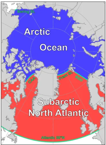
The northern polar region of Earth is mostly covered by a large water body enclosed by continents from almost all sides. This mediterranean sea is bordered by the Bering Strait from the Pacific and by the Davis Strait and the Greenland-Scotland Ridge from the Atlantic Ocean, and is often referred to as the Arctic Mediterranean. As described by Sverdrup et al. (1942), this term includes the waters of the Canadian Arctic Archipelago and Baffin Bay, as well as the Nordic Seas (a collective name for the Greenland, Iceland, and Norwegian Seas) in addition to the Arctic Ocean. Although this is considerably smaller than the definition given by the International Hydrographic Organization that includes even the Hudson Bay as part of the Arctic Ocean (IHO, 2002), this study follows its nomenclature, and considers the Arctic Ocean as the waters bounded by the Bering Strait, the Canadian Arctic Archipelago, Fram Strait, and the Barents Sea Opening.

(12)

The Subpolar North Atlantic Ocean in this study means the waters between America and Europe, bounded by the Canadian Arctic Archipelago and the Greenland-Scotland Ridge on the north, and the 50°N latitude on the south, and thus it includes the Hudson and Baffin Bays, but not the Nordic Seas. For the analysis of freshwater content and fluxes this study also uses the term Subarctic North Atlantic. This domain consists of the Subpolar North Atlantic Ocean, and the Nordic Seas and the North Sea and the Baltic Sea as well.

1.1.1. Bathymetry

The Arctic Ocean is the smallest and shallowest of the world oceans. Its bathymetry, along with the nomenclature of its most prominent features is presented on Figure 1.1. The basin of the Arctic Ocean covers an area of roughly 9.4 million km² and consists of the deep Arctic Basin, and shelf areas not deeper than 300 meters. These shelf seas are the Barents Sea, the Kara Sea, the Laptev Sea, the East Siberian Sea, and the Chukchi Sea. The deep basin is divided into the Eurasian Basin and the Canadian or Amerasian Basin by the Lomonosov Ridge, an underwater ridge that crosses the Arctic with a highest point at 1600 meters below sea level. The Eurasian Basin is further separated by the Gakkel Ridge into the 4000 meters deep Nansen Basin and the 4500 meters deep Amundsen Basin. The Amerasian Basin is also divided into two parts by the Alpha Ridge and the Mendeleyev Ridge. These are the Makarov Basin with a maximum depth of 4000 meters, and the Canada Basin, the largest and shallowest basin with a maximum depth of 3800 meters (Rudels, 2009).

The Arctic Ocean is mostly enclosed by continents and has a limited connection to other oceans. It is connected to the Pacific Ocean through the shallow (50 m) and narrow (85 km) Bering Strait. The connection to the Atlantic Ocean is through the Canadian Archipelago west of Greenland linking the Arctic Ocean to Baffin Bay and to the North Atlantic Ocean through Davis Strait (1030 m deep, 330 km wide). East of Greenland, it is connected to the Nordic Seas through the much deeper (2600 m) and wider (580 km) Fram Strait and the Barents Sea Opening (480 m deep, 820 km wide). Through these gates the Arctic Ocean exchanges water (and ice) with the world oceans (Haine et al., 2015).

The domain of the Nordic Seas is part of the Arctic Mediterranean, and is situated east of Greenland between the Arctic Ocean and the Subpolar North Atlantic Ocean (Figure 1.1). It is separated from the Arctic Ocean by the Fram Strait between Greenland and Svalbard, and by the Barents Sea Opening between Svalbard and Scandinavia. The Nordic Seas comprise the Greenland Sea, the Iceland Sea, and the Norwegian Sea, covering a total area of 2.5 million km² (Drange et al., 2005). Its deepest point, about 4800 meters underwater is located in the Greenland Sea, although on average the Norwegian Sea is the deepest, with a mean depth of about 2000 meters. The Iceland Sea is

(13)

1.1 – Main Characteristics of The Arctic and North Atlantic Oceans 3

the smallest and shallowest part of the Nordic Seas. On the south, the Nordic Seas are bound by the shallow waters of the North Sea, and on the southwest by the Greenland- Scotland Ridge that forms a natural barrier between the Nordic Seas and the Subpolar North Atlantic Ocean (Blindheim and Østerhus, 2005).

Figure 1.1. The Arctic Mediterranean and the Subpolar North Atlantic. Bathymetry data is from ETOPO1 Global Relief Model (Amante and Eakins, 2009).

The Atlantic Ocean is the second largest ocean enclosed between the American continents from the west, and Europe and Africa from the east. It is open to the south to the Southern Ocean, while in the north it is connected to the Arctic Ocean through several straits. Here focus is on its northern subpolar part and on the complex system it forms with the Arctic Ocean. The main features of its bathymetry can be seen on Figure 1.1.

The long basin of the Atlantic Ocean is divided into a western and eastern part by the Mid-Atlantic Ridge situated about 2000 meters underwater, following the border between divergent tectonic plates. The highest point of this ridge reaches a depth of 1000 meters. It acts as a divider between the deep basins on either sides, and therefore has a significant effect on the circulation of deeper waters. Both the western and the eastern basins have a depth of around 4–5000 meters, but they are shallower at higher latitudes, where their marginal seas are located. The Labrador Sea is situated in the northwest, connecting the

(14)

North Atlantic Ocean to the Arctic through Baffin Bay. It is more than 3000 m deep in the south and becomes shallower as it narrows towards Davis Strait. On the eastern side of Greenland is the Irminger Sea, bordered by Greenland, Iceland, and the northern part of the Mid-Atlantic Ridge called the Reykjanes Ridge. On the northeast the North Atlantic Ocean is open to the Nordic Seas through the Greenland-Scotland Ridge. The opening between Greenland and Iceland is called the Denmark Strait, and it has a sill depth of approximately 600 meters. The water is somewhat shallower between Iceland and the Faroe Islands (400 m), and deeper in the Faroe Bank Channel (800 m), between the Faroe Islands and Scotland.

1.1.2. Main Currents

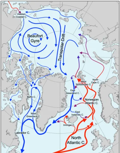
Most of the water in the Arctic Ocean is of Atlantic origin, especially the mid-depth and deep waters, but a substantial part of the water in the Amerasian Basin also comes from the Pacific Ocean. This is possible due to a network of currents transporting large volumes of water at different depths. The main surface currents of the Arctic Mediterranean and the Subpolar North Atlantic Ocean are shown on Figure 1.2.

Figure 1.2. Surface currents in the Arctic Mediterranean and in the Subpolar North Atlantic Ocean.

(15)

In the North Atlantic Ocean, warm and saline water is transported northwards by the Gulf Stream, a strong western boundary current. Reaching the latitude of about 40°N, it detaches from the American coast and turns eastwards. This part of the stream, called the North Atlantic Current, crosses the Atlantic and transports a large amount of tropical water that is significantly warmer than its surroundings towards Europe. It is characterized by a meandering flow that carries about 20 Sv (Sverdrups; 1 Sv = 10⁶ m³s^-1) of water across the Mid-Atlantic Ridge (Rossby, 1996). The North Atlantic Current forms the northern part of the subtropical gyre, a large-scale quasi-permanent anticyclonic circulation at mid-latitudes, mainly in the upper 1000 meters depth range. At the same time, it forms the southern part of the cyclonic subpolar gyre, (Schmitz, 1996).

Flowing towards Europe, the North Atlantic Current gradually weakens as other streams branch from it before it reaches the Nordic Seas. A total amount of about 8 Sv crosses between Greenland and Scotland: 1 Sv carried by the Irminger Current across Denmark Strait, and 7 Sv carried by the North Atlantic Current split between the two parts of the Iceland-Scotland Channel. Altogether, the Faroe-Scotland branch carries almost half of the water into the Nordic Seas, and it is also warmer and more saline than the others;

therefore it is the most dominant in terms of Atlantic Water import (Hansen and Østerhus, 2000).

After entering the Nordic Seas, Atlantic Water continues flowing northeast in two branches of the Norwegian Atlantic Current. Part of the eastern branch crosses the Barents Sea Opening, carrying about 2 Sv of Atlantic Water into the Arctic Ocean, where it continues as the North Cape Current (Skagseth, 2008). The rest of the eastern branch flows northwards and joins the western branch that also loses water to westward recirculating branches in the Iceland and Greenland Seas. By the time it reaches Fram Strait, the amount of Atlantic Water carried by the West Spitsbergen Current is about 3 Sv, roughly half or third of the total water flux of the current (Beszczynska-Möller et al., 2012).

Part of the Atlantic water crossing Fram Strait also recirculates westwards and joins the East Greenland Current, while most of it enters the Arctic Ocean. This warm and relatively saline surface water cools and freshens as it encounters and melts sea ice, and flows eastwards along the continental slope. It sinks underneath the cold and fresher surface water there, and continues its way northeast while joining with part of the water entering from the Barents Sea Opening that also goes through sinking as it becomes denser due to heat loss to the atmosphere and brine rejection during ice formation in winter.

Flowing further eastwards, these waters of Atlantic origin spread to large depths and reach the lower regions of the entire Arctic Basin, ultimately penetrating both the Eurasian and the Amerasian Basins (Jones, 2001; Rudels, 2009).

There is also a significant inflow of water crossing the Bering Strait, where about 1 Sv of Pacific Water enters the Arctic Ocean through the Chukchi Sea (Woodgate, 2018). This water is relatively fresh, especially in comparison with Atlantic Water, therefore it mostly

(16)

stays closer to the surface, as it continues to flow in multiple directions. Part of it enters the East Siberian Sea, its central branches penetrate the Amerasian Basin, while its easternmost part flows along the American continent as the Alaskan Coastal Current (Rudels, 2009).

The central Arctic Ocean has two main features of water flow on the surface, namely the Beaufort Gyre and the Transpolar Drift. The Beaufort Gyre is a large anticyclonic circulation cell in the Canada Basin, whose strength and extent varies greatly, as it is driven by wind forcing associated with an atmospheric pressure pattern that is dominated by alternating regimes. (Proshutinsky and Johnson, 1997). The Transpolar Drift is a surface current that transports water from the Siberian shelf seas across the Arctic towards Greenland and Fram Strait. It is also mainly wind-driven, and shows similarly large variations in its position and strength associated with patterns of atmospheric variability (Mysak, 2001). The role of atmospheric forcing is presented in detail in Chapter 1.2.3—

Atmospheric Forcing as a Driver of Freshwater Anomalies. The flow in the deeper layers of the Arctic Ocean is characterized by cyclonic circulation cells in the four deep basins.

Balancing the inflow of Atlantic and Pacific Water, there is also a southward export of cold and relatively fresh Arctic Water into the Nordic Seas and the North Atlantic Ocean. Most of the water that crosses the Arctic along the Transpolar Drift is carried into the Nordic Seas by the East Greenland Current, a strong western boundary current that transports about 11 Sv of water southwards through Fram Strait (Marnela et al., 2013). In addition to this outflow, there is also a significant export of sea ice to lower latitudes. This is discussed in Chapter 1.2—Freshwater Content and Fluxes. The top layers (down to 200 meters depth) of the East Greenland Current comprise predominantly fresh and cold Arctic Water, but at intermediate depths (200–1000 m) it carries recirculating Atlantic Water (Rudels et al., 2005). As it flows southwards, some part of it repeatedly recirculates to the east in branches in the Greenland Sea and in the Iceland Sea that are ultimately entrained in the West Spitsbergen and Norwegian Atlantic Currents. However, most of the water continues to flow southwards and enters the North Atlantic Ocean as an outflow in the top layers of about 1.3 Sv across Denmark Strait, and also as an overflow of intermediate waters of about 3-3 Sv respectively across Denmark Strait and the Iceland- Scotland Channel (Hansen and Østerhus, 2000). The East Greenland Current then continues to flow southwards until it rounds the southern tip of Greenland. There it follows the shore and turns northwards as the West Greenland Current, most of which branches westwards, while some of it continues flowing into the Baffin Bay. Here it meets Artic Water exported through the Canadian Arctic Archipelago.

Water from the Arctic Ocean that is primarily of Atlantic origin is exported through Fram Strait (and a much smaller amount through the Barents Sea Opening), while most the water of Pacific origin leaves the Arctic Ocean through the narrow and shallow

(17)

pathways across the Canadian Arctic Archipelago. The major pathways are the Nares Strait and Lancaster Sound, where fluxes are generally difficult to measure due to the harsh conditions of their remote locations. The volume flux across Nares Strait varies between 0.7–1.0 Sv, depending on the mobility of the ice cover (Münchow, 2015). The mean transport across Lancaster Sound is about 0.5–0.7 Sv (Prinsenberg et al., 2009;

Peterson et al., 2012). These, and also water from the recirculating West Greenland Current join in the Baffin Current, and flow southwards. By the time it reaches Davis Strait, this volume flux is about 1.6 Sv (Curry et al., 2014). Flowing southwards, the Baffin Current joins with the water of the West Greenland Current, and continues to flow southwards along the North American coast as the Labrador Current. After passing Newfoundland it continues to flow along the shore, while a part of it recirculates and gets entrained in the North Atlantic Current to begin its journey across the Atlantic towards the Arctic Ocean across the Nordic Seas.

1.1.3. Hydrography

The Arctic Ocean has a relatively low salinity in comparison with other oceans. This is a result of multiple sources low salinity water, or freshwater. Continental runoff from surrounding land surfaces contributes significantly to the freshness of the Arctic Ocean, since its upper layer accounts for 0.1% of the global ocean volume but receives 11% of global river discharge (Fichot et al., 2013). The inflow through Bering Strait is also relatively fresh. Moreover, in the Arctic the amount of precipitation exceeds evaporation, resulting in a net inflow of freshwater over the entire Arctic Ocean (Aagaard and Carmack, 1989).

In their fundamental study on Arctic salinity balance, Aagaard and Carmack (1989) estimated the mean salinity of the Arctic Ocean as 34.8. This value is widely accepted and used in the literature as a reference (Serreze et al., 2006). However, for a detailed investigation, the regional and vertical differences must also be considered. According to the PHC3.0 climatology of Steele et al. (2001), the largest spatial differences are observed at the surface. Excluding the immediate vicinity of major river mouths, where the surface can be almost completely fresh, the Arctic Ocean has a surface salinity between 29.5 and 35, but some of the Siberian shelf seas are even fresher. In general, the Amerasian Basin has lower surface salinity (29.5–31) than the Eurasian Basin (31–34.5), as its surface water is mostly of Pacific origin, while the latter is dominated by the inflow of high salinity Atlantic Water. The highest surface salinity is present in the Barents Sea, where its value can reach 35.

(18)

The Arctic Ocean is strongly stratified, and its water mass shows different characteristics at different depths. Rudels (2009) distinguishes five separate layers of Arctic Water:

• The Polar Mixed Layer is a 50 meters thick layer with low salinity (Amerasian Basin: 30–32, Eurasian Basin: 32–34). This upper layer is homogenized during winter by freezing, brine release and haline convection, while in summer the upper 10–20 m becomes freshened and stratified through dilution by sea ice meltwater. If forms the Polar Surface Water together with the halocline below.

• The halocline is 100–250 meters thick (thicker in the Amerasian Basin, thinner in the Eurasian Basin), and is characterized by a strong vertical gradient of salinity (32.5–34.5). Its temperature is close to freezing.

• The layer of Atlantic Water below the halocline is 400–700 meters thick with a salinity between 34.5 and 35, and a potential temperature above 0°C.

• The Intermediate Water in the deeper regions which can still cross the Lomonosov Ridge with a salinity between 34.87 and 34.92, and a potential temperature between -0.5 and 0°C.

• The deep and bottom waters fill the deepest basins. These are also of Atlantic origin, and have a salinity of between 34.92 and 34.96 and a potential temperature between -0.55 and -0.5°C in the Amerasian Basin. The typical values for the Eurasian Basin are 34.92–34.945 and -0.97– -0.5°C.

The surface waters of the Nordic Seas region are characterized by large salinity and temperature differences associated with the flow of warm and salty Atlantic Water in the southeast, and cold and fresh water exported from the Arctic along the coast of Greenland in the west. The typical surface salinity is between 32 and 35.2, with the higher values in the Norwegian Sea, and the lower values in the Greenland Sea, where the westernmost part of the East Greenland Current is even fresher than 30 near the coast. The surface temperature shows a similar pattern, with higher values up to 10°C in the southeast, and below 0°C in the northwest (PHC3.0 climatology of Steele et al. (2001)).

Atlantic Water entering the Nordic Seas through the Greenland-Scotland Channel fills some of the Iceland Sea and much of the Norwegian Sea down to a depth of about 500 meters. This Atlantic Water has a potential temperature between 7 and 10.5°C, and a salinity between 35.1 and 35.45. This water continues to flow northwards, while some of it recirculates in the Iceland and Greenland Seas, where it is situated below the top layers of cold and fresh waters of Arctic origin that have similar properties as the Polar Surface Water. From the Arctic there is also an export of deep water through Fram Strait at the depths of 1500–2500 meters. It has a potential temperature between -0.5 and -0.9°C, and a

(19)

salinity of 34.92–34.93, depending on whether it is coming from the Amerasian or the Eurasian Basin. But this is only one source of the intermediate and deep waters of the Nordic Seas, as there is also a local formation of deep water in the Greenland and Iceland Seas. Mixing together with the deep waters from the Arctic, this deep water in the Greenland Sea has a potential temperature below 0°C and salinity of 34.88–34.90. These deep waters then also fill the other deep basins of the Nordic Seas (Blindheim and Østerhus, 2005).

Deep water is formed locally in the Nordic Seas, which makes the Nordic Seas a key region for the global ocean circulation (Rudels and Quadfasel, 1991). Normally, the strong density gradients do not permit the vertical exchange of water in the ocean, thus insulating the deep ocean from the surface. Only in shelf areas at high latitudes, where the density can increase due to heat loss to the atmosphere and brine rejection during ice formation, can surface water sink to lower depths. However, there is another process, called open ocean convection. This can happen in weakly stratified water that is exposed to buoyancy loss to the atmosphere, and is characterized by a cyclonic circulation pattern that results in the doming of isopycnals. This favors the rising of weakly stratified underlying water to the surface. There it is readily exposed to intense surface forcing that in winter can significantly lower its temperature. This increases its density, so that it sinks, feeding a cycle of convection that can reach depths greater than 2000 meters (Marshall and Schott, 1999). In the Nordic Seas all the above conditions are met, and convection takes place in the Greenland and Iceland Seas. This forms deep water, which then spreads to great distances, filling the deep basins of the Arctic Ocean, and also ventilating the North Atlantic (Aagaard et al., 1985). Besides the Nordic Seas, the only location in the Northern Hemisphere where deep water formation takes place is the Labrador Sea in the North Atlantic.

The Subpolar North Atlantic Ocean is characterized by an east-west gradient of surface salinity and temperature due to the dominance of the warm and salty North Atlantic Current in the east and the cold and fresh Labrador Current in the west.

Therefore, both surface salinity and temperature are lower in the western basin, where near the coast along the Labrador Current they can be lower than 32 and 2°C, respectively.

The values quickly increase off the shore, and the typical values in the open western basin are 34–35 for salinity, and 4–9°C for temperature. In the eastern basin the surface salinity reaches 35.4 and the temperature reaches 13°C close to Ireland (PHC3.0 climatology of Steele et al. (2001)).

1.1.4. Sea Ice

The polar regions of the Earth are exposed to harsh conditions, including extremely low temperatures. At high latitudes, cold air causes the sea surface to freeze, creating a layer

(20)

of sea ice that forms at the boundary of ocean and atmosphere. Sea ice can grow to a thickness of multiple meters, and covers part of the Arctic Ocean throughout the year. Its physical properties differ from those of water, therefore it plays an important role as a mediator that can influence the interactions between ocean and atmosphere.

Ice forms when the water temperature reaches its freezing point. In clear, fresh water this is at 0°C, but in seawater with a salinity of 32, which is typical for the surface layers in the polar regions, freezing starts at -1.8°C. The ice that forms has lower salinity; while seawater freezes, most of the salt in it is rejected, leaving behind water with a high salt concentration called brine. Some salt does get trapped in the forming ice, but it gradually drains over time. Therefore, the mean salinity of younger (0.5 m thick) sea ice is around 7, and thicker multi-year Arctic ice has a salinity of about 3 (Cox and Weeks, 1974). Sea ice floats on the water surface and can drift to large distances driven by ocean currents and the wind (see Chapter 1.2.3.1—Wind Stress). When the ice melts, the meltwater is much fresher and thus lighter than the water from which the ice formed. This means that it stays on the surface, insulated from deeper waters by a strong halocline. This explains the strong stratification in the Arctic Ocean, where sea ice is forming and melting following the seasonal cycles.

The extent of sea ice, which is the area with at least 15% of ice concentration, exhibits a strong seasonal variability. This can be seen on Figure 1.3 which presents the mean ice extent of the winter maximum (blue line) and the summer minimum (orange line) in the Arctic and the North Atlantic Ocean during the period 1979–2000. In winter, sea ice covers almost the entirety of the Arctic Ocean, with the exception of a large part of the Barents Sea. There is an extensive sea ice cover in the Nordic Seas, mostly along the pathway of the Arctic sea ice export following the East Greenland Current. This can extend as far south as the southern tip of Greenland. Baffin Bay is also completely frozen over in winter, and the ice edge is in the Labrador Sea, and even further south along the continent where the cold Labrador Current dominates. In summer, most of the sea ice outside the Arctic Ocean melts. Only in the Canadian Arctic Archipelago and in the western Greenland Sea some ice remains. Within the Arctic Ocean, the ice also melts along the continents and in some of the shelf seas, while the central Arctic has a permanent, year-round ice cover. Due to the lack of seasonal melt, this ice is thicker, as it can be seen on Figure 1.3 that also shows the mean sea ice thickness for March in the period 2011–2017. The thickest ice is observed north of the Canadian Arctic Archipelago and Greenland, where it extends to 3.5 meters, but a large part of the central Arctic has an ice cover thicker than 2 meters. In the shelf seas the typical maximum thickness is 1–1.5 meters, except for the Kara Sea (0.5–1 m) and the Barents Sea which is mostly ice-free even in winter. The ice exported through Fram Strait contains a large amount of multiyear ice, therefore the mean thickness is rather high (up to above 3 m) along the East Greenland Current. In other lower latitude seas, the thickness usually does not exceed 1 meter.

(21)

Figure 1.3. Arctic and North Atlantic sea ice cover. The lines contour the average winter maximum (blue) and summer minimum (orange) extent of sea ice during the period 1979–2000 based on data from the National Snow and Ice Data Center. The map shows average March sea ice thickness during the period 2011–2017 based on CryoSat-2/SMOS data downloaded from www.meereisportal.de (Grosfeld et al., 2016).

The seasonal changes and time series of sea ice extent in the Northern Hemisphere are plotted on Figure 1.4. The large seasonality is clearly visible on the left panel, as the maximum extent in March (almost 16 million km²) is twice the size of the September minimum (7.3 million km²). The right-side panel depicts temporal changes of the March maximum and the September minimum from 1979 until 2016. Both show a decreasing trend that is also stronger in the last two decades than before. The summer extent has been declining at a higher rate than the winter extent. Overall, observations show that Arctic sea ice is retreating, with less ice forming in winter, and more ice melting during summer, as the same reduction has been observed for the ice thickness and thus the total volume of the ice (Kwok et al., 2009).

(22)

Figure 1.4. Sea Ice Extent in the Northern Hemisphere. Left: seasonal cycle averaged over 1979–

2010. Right: time series of March and September means. Data is based on EUMETSAT OSI SAF ice concentration (Tonboe et al., 2016).

The strong seasonal cycle of sea ice influences the salinity of the upper water layers as the process of freezing extracts freshwater from the ocean, while the melting provides a source of it. Sea ice can drift to great distances and can melt in a different region than where it was formed, thus it also plays an important role as a freshwater vector in the ocean. The following chapter introduces the concept of oceanic freshwater content, and reviews the state of the art of its research in the Arctic and North Atlantic Oceans.

1.2. Freshwater Content and Fluxes

The salinity of a water solution can be modified by adding or subtracting either salt or water. In the world oceans the total amount of salt varies very little and only very slowly, and therefore can be considered constant even on millennial time scales. Although the total volume of water can change faster by the build-up and melt of great ice sheets during glacial and interglacial periods, they can be ignored here as this study investigates variability in decadal time scales, over which these processes are not significant. On decadal time scales the total volume of water is also very stable due to a global balance of sources (river runoff and precipitation) and sinks (evaporation). However, on a regional scale these are often not balanced.

In the North Atlantic Ocean evaporation exceeds precipitation, removing freshwater and thus increasing salinity. In the Arctic Ocean it is the other way around; river runoff and precipitation supply much more freshwater than what is removed by evaporation, contributing to a low salinity. These differences are somewhat balanced by the exchange of water. The transport of Atlantic Water brings saltier water into the Arctic Ocean, from where fresher Arctic Water is exported to the North Atlantic. Local variations in the salinity, especially in the upper layers, are thus driven by changes associated with river runoff, precipitation, evaporation, oceanic currents—fluxes of water. That is why it is

(23)

1.2 – Freshwater Content and Fluxes 13

useful to define a metric for salinity that makes the contribution of these sources and sinks easier to assess. This metric is the oceanic freshwater content.

1.2.1. Concept

The general concept of oceanic freshwater content is that the salinity of a volume of sea water is described by how much freshwater is stored in it, including the amount stored in sea ice. These two phases (liquid and solid freshwater content) are investigated separately in this study, because of the differences in their variability and their driving forces.

Liquid freshwater content is the amount of zero salinity water that is required to reach to observed salinity of a volume of seawater starting from a reference salinity. It is essentially an alternate metric for salinity, and does not assume a body of actual freshwater within the seawater, but illustrates how much fresher or saltier the sample of seawater is compared to a reference salinity. Freshwater content can also be negative, when the sample is saltier than the reference. It is a useful metric because freshwater anomalies have a very limited effect on the mean salinity even locally, but they play an important role in a wide range of physical and biogeochemical processes in the ocean with local and global consequences. A few examples are stratification, vertical mixing, deep convection, ocean heat flux, sea ice formation, and also nutrient supply, primary production, ocean acidification (Carmack et al., 2016).

Liquid freshwater content (𝐿𝐹𝑊𝐶) in a volume of water with a surface 𝐴 and depth 𝑧 can be calculated according to the following formula:

𝐿𝐹𝑊𝐶 = ( ) 𝑆_+,-− 𝑆 𝑆_+,- 𝑑𝑧 𝑑𝐴

1

234 5 (1.1)

where the vertical integration is from the surface (𝑧 = 0 m) down to depth level ℎ, 𝑆 is the observed salinity, and 𝑆_+,- is the reference salinity. Similarly, the freshwater flux (𝐿𝐹𝑊𝐹) across an oceanic section 𝐴 is defined as the equivalent flux of zero salinity water, and is given by

𝐿𝐹𝑊𝐹 = ) 𝑣𝑆_+,-− 𝑆

𝑆_+,- 𝑑𝐴 (1.2)

where 𝑣 is the velocity component normal to the section 𝐴.

As it is apparent from both Equations (1.1) and (1.2), the value of freshwater content and flux depend on the choice of ℎ and 𝑆_+,-. While calculating the freshwater content, ℎ is usually selected as the depth where 𝑆 = 𝑆_+,-., therefore the integration in the vertical is done in the upper layers where the salinity is lower than the reference. In this case the

(24)

freshwater content is non-negative. Another common value for ℎ is the full depth of the water column. In this case the freshwater content can be negative as well, when 𝑆 > 𝑆_+,-in a large part of the water column. The choice of 𝑆_+,- affects both the freshwater content and fluxes as well. In their fundamental study of Arctic freshwater content, Aagaard and Carmack (1989) used 𝑆_+,- = 34.8 based on an approximate value of mean Arctic salinity.

This is the most commonly used reference (Serreze et al., 2006), although there are studies that use different values for the freshwater content, such as for example 35.0 (Rabe et al., 2014) and for the fluxes, for example 34.9 (Holfort and Meincke, 2005) or 35.2 (Dickson et al., 2007).

The impact of the applied reference salinity is particularly important for the calculation of freshwater fluxes. According to Tsubouchi et al. (2012), the ideal choice is to use a reference salinity that equals to the mean salinity of the investigated ocean basin.

Although an arbitrary 𝑆_+,- in the denominator of Eq. (1.2) violates the conservation of mass, this leads to an insignificant error while calculating the total net flux for an enclosed region. This is because when all the boundaries are considered in the integration, an underestimation in one direction is compensated by an overestimation in another direction. In this case, the range of error in the total net freshwater flux arising from using different reference values (within reasonable limits, for example 34.8 < 𝑆_+,- < 35.2) is within 1%, and therefore can be ignored. But as pointed out by Tsubouchi et al. (2012), there is no compensation for the error when a single freshwater flux is calculated across a section, and in that case reference salinity must be chosen with care. The ideal choice is the mean salinity of the investigated flux, which varies from section to section.

The amount of freshwater stored in sea ice is referred to as solid freshwater content.

Its value depends on the volume and the age of the ice, as generally the salinity of frozen seawater is gradually declining over time as it continues to grow (Cox and Weeks, 1974).

Likewise, drifting sea ice is considered a solid freshwater flux.

1.2.2. Observed mean values

A complete freshwater budget of the Arctic Ocean is provided by Haine et al. (2015). As they state in their introduction, the global cycle of water in the atmosphere is characterized by a high rate of evaporation in the tropics, a transport of moisture to higher latitudes, and precipitation in the polar regions. This makes the Arctic Ocean a terminus of the atmospheric water circulation, which leads to the accumulation of freshwater.

(25)

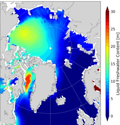
Figure 1.5. Liquid freshwater content (Sref = 34.8, integrated from surface down to Sref) in the Arctic Ocean and in the Subarctic North Atlantic. Calculated from salinity data from PHC3.0 climatology (Steele et al., 2001).

The Arctic Ocean (plus Baffin Bay) holds about 93,000 km³ of liquid freshwater relative to a reference salinity of 34.8 (Haine et al., 2015). The spatial distribution of this amount is depicted on Figure 1.5, which shows the thickness of a freshwater layer whose volume is equivalent to the freshwater content integrated in the water column below. Most of the liquid freshwater is stored in the Amerasian Basin, where values reach 18 meters in the Beaufort Gyre, a major reservoir of freshwater. Although their surface salinity is lower, the shelf seas contain much less freshwater due to their shallow depths. There are lower values in the Eurasian Basin too (2–9 m), due to the dominance of high salinity Atlantic Water inflow. Most of the Subarctic North Atlantic contains no freshwater, as the local surface salinity is higher than 34.8. Only along the export pathway of Arctic Water is some freshwater present, for example along the East Greenland Current (2–10 m) and in the coastal regions of the Labrador Sea (3–12 m).

(26)

Mean values for 1980–2000 Freshwater content [km³]

Liquid 93,000

Solid 17,800

Net freshwater flux [km³yr^-1]

River runoff 3900 ± 390

Precipitation - Evaporation 2000 ± 200 Bering Strait liquid 2400 ± 300 Bering Strait solid 140 ± 40

Greenland ice melt 330 ± 20

Davis Strait liquid -3200 ± 320

Davis Strait solid -160 ± ?

Fram Strait liquid -2700 ± 530

Fram Strait solid -2300 ± 340

Barents Sea Opening -90 ± 90 Fury and Hekla straits -200 ± ?

Total fluxes [km³yr^-1]

Inflow sources 8800 ± 530

Outflow sinks -8700 ± 700

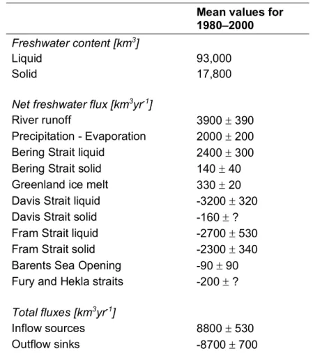
Table 1. Freshwater budget of the Arctic Ocean relative to a reference salinity of 34.8.

Negative values indicate southward transport. From Haine et al. (2015).

The contribution of the solid component (sea ice) in most parts of the Arctic Ocean is smaller. On average there is about 17,800 km³ of freshwater stored in sea ice (Haine et al., 2015). Assuming an average salinity of 5, the freshwater content of a 1 meter thick ice is 0.76 meters. Considering the typical mean ice thickness of 1–2 meters, this translates to a 0.7–1.5 meters thick layer of freshwater, which is about an order of magnitude smaller than the liquid component.

The individual components of sources and sinks of Arctic freshwater are listed in Table 1. The largest source of freshwater is river runoff, discharging about 3,900 km³ of freshwater into the Arctic Ocean per year. In the Arctic, precipitation exceeds evaporation;

their net rate yields a freshwater supply of 2,000 km³yr^-1. Considering the lateral fluxes, the inflow of Pacific Water through Bering Strait carries 2,400 km³of freshwater annually.

Together with a few minor components, the total inflow adds up to about 8,800 km³yr^-1. Balancing this inflow, there is a significant export of freshwater from the Arctic to lower latitudes, into the Nordic Seas and the North Atlantic Ocean. The largest outflow component is the liquid freshwater flux through Davis Strait, about 3,200 km³yr^-1. The solid component in this section is not significant (160 km³yr^-1). The other major export pathway is on the eastern side of Greenland, through Fram Strait. Here the liquid component (2,700 km³yr^-1) is comparable to that of the Davis Strait, but the total export is

(27)

even higher, as Fram Strait is the main gateway for the Arctic sea ice export. Together with the solid component the total freshwater flux is about 5,000 km³yr^-1. The sum of freshwater sinks, including those through the Barents Sea Opening and some further minor sections in the Canadian Arctic Archipelago, is about 8,700 km³yr^-1.

Comparing the sources and the sinks a dynamic balance is apparent. However, it must be noted that the harsh conditions of the above locations make observations challenging, and in some cases they have considerable uncertainties. Furthermore, all the above freshwater content and fluxes are mean values for the period 1980–2000. As reviewed by Haine et al. (2015), the observational estimates for 2000–2010 show significant changes. This is particularly true for the solid components that show a negative trend due to the gradually shrinking Arctic sea ice cover. River runoff and precipitation are increasing. Recent observations suggest that the sources increased and the sinks decreased in the period of 2000–2010, with a residual of 1,200 km³yr^-1 freshening the Arctic Ocean.

In recent decades there has been a growing interest in observing and also modeling the Arctic Ocean freshwater budget, and the anomalies of its components. The variabilities of the system have been the focus of many studies, but there is still much that is not understood. What is the relationship of the Arctic freshwater system to anomalies observed in the Subarctic North Atlantic, its main export target? What are the key physical processes governing Arctic freshwater storage and release? In particular, what are the driving forces of the observed anomalies? The next chapter briefly reviews the state of the art in Arctic and North Atlantic freshwater research with a focus on wind stress forcing associated with large-scale modes of atmospheric variability.

1.2.3. Atmospheric forcing as a driver of freshwater anomalies

1.2.3.1. Wind stress

Air-sea interactions play a critical role in the climate system. Winds with a characteristic horizontal speed two orders of magnitude higher than that of the water surface below exert a strong momentum forcing on the ocean due to friction. This wind stress forcing drives an ocean circulation from local to global scales (Munk, 1950).

During his pioneering Arctic expedition, Nansen (1902) noted that the speed of sea ice drift was 2% of the wind speed, and its direction deviated to the right from the wind direction. Motivated by these observations, Ekman (1905) described the physics of the wind-driven transport near the ocean surface as the effect of wind forcing, ice-water stress, and the Coriolis force. This atmospheric momentum forcing can be estimated by a quadratic drag formula. According to Yang (2006), when wind directly blows over the water, the air-water stress is described by

(28)

𝜏_; = 𝜌_;𝐶₌|𝑢_;@|(𝑢_;@) (1.3)

where 𝜌_; is the density of air (1.25 kgm^-3) and 𝐶₌ is a drag coefficient (0.00125). The term 𝑢_;@ is the relative velocity between the wind and the water at the surface: 𝑢_;@ = 𝑢_;C+− 𝑢_@;D,+. As 𝑢_@;D,+ is much smaller than 𝑢_;C+, it can be ignored for large-scale studies (but should be taken into account for coastal currents, in fronts, and in some channels and straits).

The formula is different when sea ice is present. In this case, it is not the air, but the sea ice that directly drags the water. The ice-water stress is described by

𝜏_C= 𝜌_@𝐶_C@|𝑢_C@|(𝑢_C@) (1.4)

where 𝜌_@ is the water density, 𝐶_EC is a drag coefficient (0.0055). The relative velocity in this case is between the ice and the surface water: 𝑢_C@= 𝑢_CF,− 𝑢_@;D,+. Here 𝑢_@;D,+ must not be ignored, as its characteristic values are comparable to those of 𝑢_CF,.

In the Arctic Ocean, the water surface is often not fully ice-free or completely frozen over; sea ice concentration (𝛼) can vary between 0 and 100%. Therefore, the total surface stress can be written as

𝜏 = 𝛼𝜏_C+ (1 − 𝛼)𝜏_; (1.5)

The effect of wind stress on the velocity in the Ekman layer, which is the upper water column where the effect of wind stress forcing is the most dominant, is calculated by the following equations:

−𝑓𝑣_KL = 𝜏_M

𝜌𝐷_K 𝑎𝑛𝑑 𝑓𝑢_KL = 𝜏_Q

𝜌𝐷_K (1.6)

where 𝑓 is the Coriolis parameter (𝑓 = 2Ω𝑠𝑖𝑛𝜑, Ω is the rotation rate of the Earth, 𝜑 is the geographical latitude), about 1.45 x 10^-4 s in the Arctic Ocean. The parameter 𝐷_K is the Ekman layer depth, typically around 20 meters in the Arctic Ocean (Hunkins, 1966). As the wind stress and the Ekman velocity are co-dependent, the equations (1.3), (1.4), and (1.6) are solved iteratively.

The wind-driven Ekman transport occurs at an angle to the wind forcing. In the Northern Hemisphere, the transport vector deviates about 45° to the right at the surface, and about 90° in the total vertical column of the Ekman layer. This means that the curl in the forcing wind field creates vertical motion. Negative wind stress curl in an anticyclone leads to convergent Ekman transport. Convergent water domes and is also pushed

(29)

downwards. This wind-driven vertical motion is called Ekman pumping. The opposite is called Ekman suction, when the divergent Ekman transport leads to upwelling in the upper water layers. The rate of this vertical motion (𝑤_KL) depends on the curl of the wind stress:

𝑤_KL=(∇ × 𝜏)

𝜌𝑓 (1.7)

where 𝜌 is the density of the water and 𝑓 is the Coriolis parameter.

Wind on a small scale is rather turbulent, but on a larger scale it follows the spatial trends of sea level pressure, driven by a geostrophic balance between the pressure gradient force and the Coriolis force. The large, basin-scale wind-driven structures in the ocean are driven by these geostrophic winds; therefore, for the investigation of wind- driven anomalies in the ocean, the understanding of the large-scale variability of atmospheric sea-level pressure is essential.

1.2.3.2. Large-scale Atmospheric Variability

Features of the large-scale atmospheric variability are presented through variations of sea-level pressure, due to its relevance for geostrophic winds that drive the basin-scale transport of upper layer waters in the ocean. Although variations of sea-level pressure show no particular periodicity, there are certain hemispheric patterns of its dominant modes. These often resemble teleconnections between different centers of action, and are described by oscillation indices. In the Northern Hemisphere, the most robust are the Arctic Oscillation (AO) and the North Atlantic Oscillation (NAO).

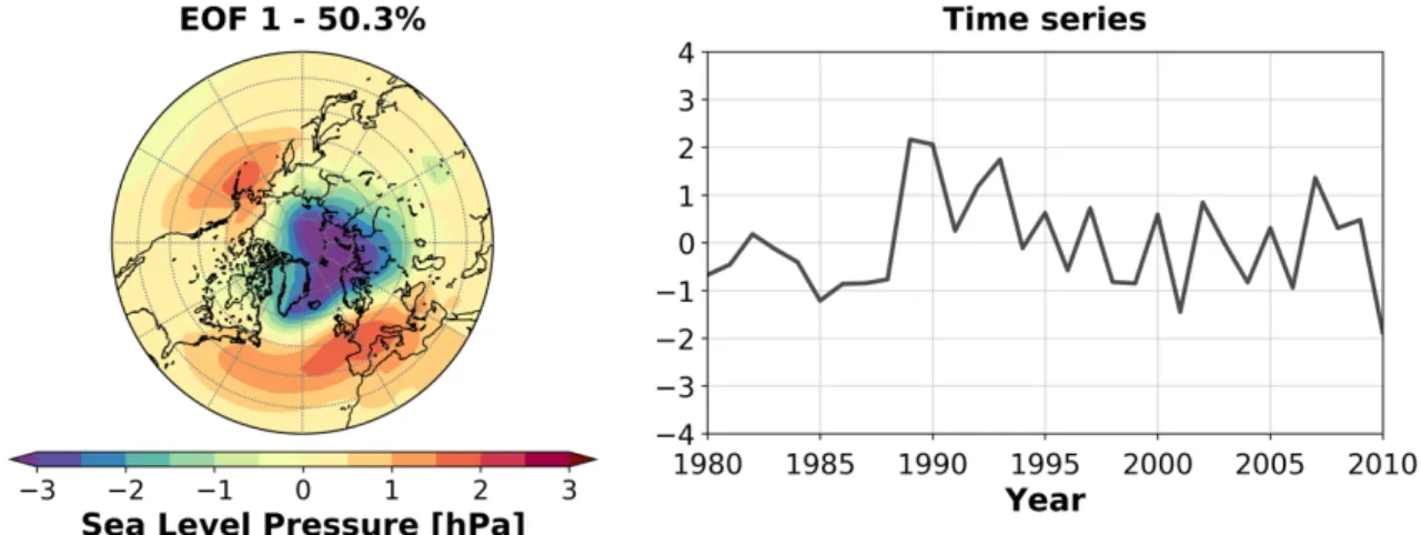
The AO is the main mode of variability in the Arctic troposphere that strongly affects Arctic circulation. In this study, the AO was calculated following the definition of Thompson and Wallace (1998): it was based on a principal component analysis or an Empirical Orthogonal Function analysis (EOF; see details in the Appendix) of the detrended November–April seasonal mean sea-level pressure anomaly field north of 20°N. Its pattern and time series are presented on Figure 1.6. The AO is characterized by a pattern of sea level pressure that has a center of action over the Arctic Ocean, and counterparts of opposite sign at lower latitudes in the Northern Pacific and Atlantic. This pattern can be interpreted as the surface signature of the variations in the polar vortex. Its strength is described by and index, whose time series show high correlations with hemispheric geopotential height and Eurasian surface air temperature anomalies on an interannual time scale (Thompson and Wallace, 1998).

During the negative phase of the AO, air pressure is high across the Arctic, which is associated with a strong Beaufort High, a prominent anticyclone over the Amerasian

(30)

Basin. This leads to the strengthening of the Beaufort Gyre that can store freshwater more efficiently due to enhanced Ekman transport from stronger anticyclonic winds inflating it.

River runoff from Siberia is directly transported towards Fram Strait by a strong Transpolar Drift. During a positive phase of the AO, air pressure is lower in the Arctic.

Siberian river runoff is brought towards the Amerasian Basin before leaving the continental shelf. At the same time, stored freshwater volume reduces in the Beaufort Sea, as the Beaufort Gyre is typically weaker (Mauritzen, 2012). As Haine et al. (2015) concludes, these processes suggest that the AO and the Beaufort High control the interannual variability of the freshwater system. The surface circulation redistributes freshwater by changing its pathways and residence times: the AO determines the freshwater source and delivery to the Amerasian Basin while the Beaufort High determines the freshwater storage of the Beaufort Gyre. This is consistent with the Arctic liquid freshwater content anomalies reported by Rabe et al. (2014), as their time series show a high correlation with the so-called Arctic Ocean Oscillation, a measure for the wind stress curl in the Arctic (Proshutinsky and Johnson, 1997). This suggests that the changes in Arctic liquid freshwater content are connected to regional changes in sea-level pressure fields rather than hemispheric-scale changes described by the AO.

Figure 1.6: Arctic Oscillation (AO) for winter (November–April) in NCEPcfsr reanalysis (Saha et al., 2010) as the (left) eigen vector and (right) principal component time series of the first empirical orthogonal function (EOF) of Northern Hemispheric sea-level pressure for the period 1980–2010.

The Arctic Oscillation is closely related to the atmospheric pressure differences of the North Atlantic that also show a distinct pattern (Figure 1.7). This is called the North Atlantic Oscillation, a major source of low-frequency atmospheric variability in the North Atlantic that describes the co-variability of the strength of the Icelandic Low and the Azores High (Hurrell, 1995).

There are different methods to calculate an index that describes the North Atlantic Oscillation, but they are similar in that they derive the NAO index from normalised sea- level pressure time series of the North Atlantic sector (Greatbatch, 2000). Here it was

(31)

calculated following Hurrell et al. (2003) as the leading EOF mode of sea-level pressure variability in the region 20°N–70°N, 90°W–40°E (Figure 1.7). This method uses detrended sea-level pressure anomalies of the winter season (mean of December–February), as this teleconnection is present throughout the year, but its effects are most significant in winter (Barnston and Livezey, 1987).

Figure 1.7: North Atlantic Oscillation (NAO) for winter (December–February) in NCEPcfsr reanalysis (Saha et al., 2010) as the (left) eigen vector and (right) principal component time series of the first empirical orthogonal function (EOF) of Northern Hemispheric sea-level pressure for the period 1980–2010.

The variability of the NAO influences the climate of the North Atlantic region, the underlying ocean, and the surrounding continents on interannual to decadal time scales (Marshall et al., 2001). The NAO can be interpreted as a measure of the strength of the westerly winds blowing across the North Atlantic Ocean. A high NAO situation means stronger than average westerly winds that especially in winter cause a negative temperature anomaly in the Canadian Arctic, and bring warmer than normal conditions over the Eurasian continent (Greatbatch, 2000). The NAO has a significant impact on oceanic processes as well. The long-term fluctuations of the sea surface temperature (SST) of the North Atlantic region correspond to atmospheric fields of sea-level pressure and surface winds (Kushnir, 1994). The NAO influences convection and deep water forming in the North Atlantic Ocean and the Nordic Seas (Dickson et al., 1996), as well as the North Atlantic gyre circulation (Curry and McCartney, 2001; Bersch et al., 2007). It also affects the transport of Atlantic Water into the Arctic, and affects temperature, salinity, sea ice cover, and thus freshwater in the Arctic Ocean (Dickson et al., 2000; Kwok, 2000).

The AO and the NAO have a high temporal correlation and are nearly indistinguishable (Deser, 2000). Considering their structure and applicability, the statistical arguments of Huth (2007) suggest that for interpreting the hemispheric circulation variability, the NAO should be preferred. Other studies also suggest that the AO is a rather statistical artifact, and the NAO is more physically consistent (Ambaum et

(32)

al., 2001), although the non-winter AO might be a true teleconnection separate from the NAO (Rogers and McHugh, 2002). Either AO or NAO, the large-scale wind variations are strongly associated with patterns of atmospheric sea-level pressure variability. The corresponding changes in oceanic circulation can among others impact salinity and sea ice, thus ultimately the freshwater content. The following chapter presents the state of the art of the research in the anomalies of Arctic and North Atlantic freshwater with a focus on their wind stress forcing associated with the above patterns of atmospheric variability.

1.2.3.3. Freshwater anomalies and the role of wind stress forcing

Observations from recent decades show significant anomalies in the freshwater content of the Arctic Ocean (Rabe et al., 2014) and also the Subarctic North Atlantic (Boyer et al., 2007). The anomalies in these two domains have a corresponding size and time scale.

Moreover, the annual amount of freshwater communicated between their basins mostly through Fram Strait (Spreen et al., 2009; Rabe et al., 2013) and the Canadian Arctic Archipelago and Davis Strait (Curry et al., 2014) is also of similar order.

Synthetizing previous studies, (Aagaard and Carmack, 1989) created the first complete freshwater budget of the Arctic Ocean, and discussed its role in the regional and global circulation. The following advances in research were summarized by Serreze et al.

(2006) combining terrestrial and oceanic observations, reanalysis data, and model results of Arctic freshwater, and by Dickson et al. (2007) reviewing the observations of its fluxes through the Arctic Ocean and subarctic seas. An overview of the growing attention to Arctic freshwater is presented by recent reviews focusing on its export to lower latitudes (Haine et al., 2015), on its role in the marine system (Carmack et al., 2016), and on modeling activities in its research (Lique et al., 2016).

Studies on the mechanisms controlling Arctic freshwater storage suggest the importance of wind stress forcing. Modeling the response of the Arctic Ocean to changes in atmospheric sea-level pressure, Proshutinsky and Johnson (1997) identified two wind- driven circulation regimes alternating with a period of 10-15 years. During an anticyclonic regime freshwater accumulates in the Beaufort Gyre, and it is released during a cyclonic regime (Proshutinsky et al., 2002). This is due to the varying strength of the Ekman pumping of freshwater, dependent on the wind field associated with the strength of the Beaufort High, a prominent anticyclone over the Amerasian Basin (Serreze and Barrett, 2011). The strength of the Beaufort High is also associated with the AO. In the Atlantic sector the AO is represented by the NAO, to which variations of Arctic freshwater have also been linked (Dickson et al., 2000). The effects of the AO and the NAO are rather similar since they are closely related (Deser, 2000). Overall, freshwater distribution in the Arctic Ocean is controlled by the combined effect of these features. The source of

(33)

freshwater and its pathways are determined by the AO, while the rate of its accumulation in the Beaufort Gyre depends on the strength of the Beaufort High (Mauritzen, 2012).

Proshutinsky et al. (2002) hypothesized a connection between Arctic freshwater content and export driven by atmospheric circulation regimes. It has been confirmed that the storage and export of both Arctic sea ice and liquid freshwater are linked and they are influenced by said regimes reminiscent of the AO (Zhang et al., 2003) and the NAO (Condron et al., 2009). Recent coupled model studies suggest their relationship and its link to atmospheric forcing. According to Lique et al. (2009) there is no significant correlation between liquid freshwater fluxes across the two pathways, although their volume transports are strongly anti-correlated. Jahn et al. (2010) showed that liquid freshwater export though the Canadian Arctic Archipelago and Fram Strait follow Arctic atmospheric circulation changes associated with the AO in 1 and 6 years, respectively, and discussed the major role that large-scale wind forcing plays by modifying sea surface height and freshwater content upstream in the Arctic. Wang et al. (2017) found this forcing to be associated with the fluxes being out of phase in the Canadian Arctic Archipelago and Fram Strait.

Changes in Arctic freshwater export can be connected to anomalies in lower latitudes.

Variabilities in the Nordic Seas and the Subpolar North Atlantic Ocean are characterized by major freshening episodes in recent decades (Curry and Mauritzen, 2005), the first of which happened in the 1970s and was named the Great Salinity Anomaly (GSA) by Dickson et al. (1988). Aagaard and Carmack (1989) reported that the origin of this event must have been an anomalously large Arctic freshwater (both sea ice and liquid) discharge through Fram Strait. This was confirmed by Häkkinen (1993) using a coupled ocean-sea ice model, who also identified high latitude wind field changes as a source of this discharge anomaly. The 1970s GSA was followed by similar events in the 1980s (Belkin et al., 1998) and the 1990s (Belkin, 2004). According to Haak et al. (2003), these anomalies were also a result of an excess of Arctic freshwater export mainly through Fram Strait due to wind forcing. Karcher et al. (2005) also linked the 1990s GSA to an increased freshwater export through Fram Strait, and showed that it was a response to the prolonged high NAO state of the early 1990s.

But even if the link between the Arctic and the Subarctic North Atlantic freshwater contents is accepted, it is still not clear what drives the redistribution within their joint system, as its response to atmospheric forcing on a longer time scale is still not fully understood. The freshwater content of the Beaufort Gyre seems to have stabilized at a high level in recent years (Zhang et al., 2016), concurrent with an unusually long anticyclonic circulation pattern in the Arctic (Proshutinsky et al., 2015). Some studies found that an eventual switch to a cyclonic regime could result in its release, possibly causing another GSA (Giles et al., 2012; Stewart and Haine, 2013). Past GSAs have mostly been associated with changes in large-scale Arctic circulation, especially in the wind field over the Beaufort

(34)

Gyre, but this link is still not clearly understood. For example, the 1970s event occurred during an anticyclonic regime, and as Dickson et al. (2000) concludes, an anomalous freshwater export from the Arctic can occur during both extrema of the NAO.

Nevertheless, the size and timing of observed freshwater anomalies in the Arctic Ocean and in the Subarctic North Atlantic during the last 20 years might suggest a multidecadal oscillation between their basins (Horn, 2018), although it is difficult to assess due to the still too short history and the uncertainty of observations. The fluxes between their basins are also particularly difficult to measure. To overcome these limitations there have been successful attempts at simulating their freshwater content with forced ice-ocean models (e.g. Häkkinen, 1993; Gerdes and Koberle, 1999; Haak et al., 2003; Karcher et al., 2005; Gerdes et al., 2008; Stewart and Haine, 2013), but still not sufficient research has been done considering them together as a joint system using fully coupled models with a dynamic atmospheric component.