JournalofGeophysicalResearch:Oceans PUBLICATIONS

(1)

RESEARCH ARTICLE

10.1002/2014JC010384

The impact of mean state errors on equatorial Atlantic interannual variability in a climate model

Hui Ding¹, Noel Keenlyside², Mojib Latif^1,3, Wonsun Park¹, and Sebastian Wahl¹

1GEOMAR Helmholtz Centre for Ocean Research Kiel, Kiel, Germany,²Geophysical Institute, University of Bergen and Bjerknes Centre for Climate Research, Bergen, Norway,³University of Kiel, Kiel, Germany

Abstract

Observations show that the Equatorial Atlantic Zonal Mode (ZM) obeys similar physics to the El Ni~no Southern Oscillation (ENSO): positive Bjerknes and delayed negative feedbacks. This implies the ZM may be predictable on seasonal timescales, but models demonstrate little prediction skill in this region. In this study using different conﬁgurations of the Kiel Climate Model (KCM) exhibiting different levels of systematic error, we show that a reasonable simulation of the ZM depends on realistic representation of the mean state, i.e., surface easterlies along the equator, upward sloping thermocline to the east, with an equatorial SST cold tongue in the east. We further attribute the differences in interannual variability among the simulations to the individual components of the positive Bjerknes and delayed negative feedbacks. Differ- ences in the seasonality of the variability are similarly related to the impact of seasonal biases on the Bjerknes feedback. Our results suggest that model physics must be enhanced to enable skillful seasonal predictions in the Tropical Atlantic Sector, although some improvement with regard to the simulation of Equa- torial Atlantic interannual variability may be achieved by momentum ﬂux correction. This pertains especially to the seasonal phase locking of interannual SST variability.

1. Introduction

The zonal mode (ZM) or Atlantic Ni~no dominates interannual variability in the Equatorial Atlantic [Xie and Carton, 2004;Zebiak, 1993]. ZM events primarily peak in boreal summer, but similar variability is also found in November–December [Okumura and Xie, 2006]. Associated sea surface temperature (SST) anomalies can exceed 1C in the eastern Equatorial Atlantic (20W and 0W, 3S and 3N). Equatorial Atlantic variability has major socioeconomic impacts, exerting a significant influence on surrounding countries [Folland et al., 1986;Carton and Huang, 1994;Nobre and Srukla, 1996;Chang et al., 2006]. Recently, the ZM was also shown to even influence the El Ni~no Southern Oscillation (ENSO) in the Tropical Pacific [Jansen et al., 2009;Losada et al., 2009;Wang, 2006;Wang et al., 2009;Rodrıguez-Fonseca et al., 2009;Ding et al., 2011] and has the potential to improve ENSO prediction skill [Frauen and Dommenget, 2012;Keenlyside et al., 2013].

Numerous studies [e.g.,Zebiak, 1993;Keenlyside and Latif, 2007] have shown that the zonal mode resembles ENSO in the Tropical Paciﬁc, suggesting that it may arise from similar coupled ocean-atmosphere interaction. The Bjerknes positive feedback, involving equatorial zonal winds, SST, and upper ocean heat content is prominent in the structure of peak phase anomalies in observations and reanalysis [e.g.,Ruiz-Barradas et al., 2000;Ding et al., 2010]. However, each of its three elements explains less variance than in the Paciﬁc [Keenly- side and Latif, 2007]. Furthermore, several studies [Zebiak, 1993;Wang and Chang, 2008;Jansen et al., 2009;

Ding et al., 2010] have shown that a delayed negative feedback involving a recharge of the upper ocean heat content plays an important role in the Equatorial Atlantic variability. Other mechanisms for SST variability may also exist in the Equatorial Atlantic [Narvaez et al., 2003;Richter et al., 2012], but here we concentrate on the ZM.

The simulation of Equatorial Atlantic variability deserves more attention [Mu~noz et al., 2012;Liu et al., 2013;

Richter et al., 2014a] given that almost all state-of-the-art coupled general circulation models (CGCM) exhibit a large warm bias in the climatological eastern Tropical Atlantic SST [e.g.,Richter and Xie, 2008;Wahl et al., 2009;Richter et al., 2014a;Wang et al., 2014].Mu~noz et al. [2012] analyze Tropical Atlantic variability from simulations of the fourth version of the Community Climate System Model (CCSM4). Their results show that the CCSM4 captures Atlantic Ni~no in terms of the leading rotated empirical orthogonal function (EOF) of

Key Points:

A reasonable simulation of Atlantic Nino depends on realistic mean state

Model physics must be enhanced to enable skillful predictions of Atlantic Nino

Correspondence to:

H. Ding, hding@geomar.de

Citation:

Ding, H., N. Keenlyside, M. Latif, W. Park, and S. Wahl (2015), The impact of mean state errors on equatorial Atlantic interannual variability in a climate model, J. Geophys. Res. Oceans,120, 1133–

1151, doi:10.1002/2014JC010384.

Received 13 AUG 2014 Accepted 16 JAN 2015

Accepted article online 27 JAN 2015 Published online 23 FEB 2015

Journal of Geophysical Research: Oceans

PUBLICATIONS

(2)

Tropical Atlantic SST anomalies even though there are signiﬁcant SST bias. Furthermore, bothLiu et al.

[2013] andRichter et al. [2014a] investigate the simulations of Atlantic Ni~no in terms of the models partici- pating in the Coupled Model Intercomparison Project Phase 5 (CMIP5).

Theoretical and observational studies indicate that the mean state has a strong control on interannual variability in the Tropical Pacific [e.g.,Battisti and Hirst, 1989;Fedorov and Philander, 2001;L€ubbecke and McPha- den, 2013]. However, it is still not clear what is the influence of the warm bias on the interannual variability in the Equatorial Atlantic given that some coupled model can capture Atlantic Ni~no while others cannot, as reported in recent studies [Mu~noz et al., 2012;Liu et al., 2013;Richter et al., 2014a]. Can simulation of interannual variability be improved in a CGCM if the bias is reduced? In particular, what is the influences of the warm bias on the mechanism of Atlantic Ni~no? There are practical interests to address these questions. For instance,Stockdale et al. [2006] investigated the prediction skill of Equatorial Atlantic variability in six CGCMs (from the EU-DEMETER project) and found that none of them show skill. The warm bias may be partly responsible for low decadal forecast skill in the Tropical Atlantic [Smith et al., 2007;Hazeleger et al., 2012;

Guemas et al., 2013].

Here we address the questions presented above by investigating a set of experiments conducted with a CGCM with perturbed parameters and momentum ﬂux correction. In section 2, we brieﬂy describe the data, model, experiments, and mean states. In section 3 and 4, we present the results and a summary and discussion of the main results, respectively.

2. Data, Model, Experiments, and Mean States

Sea surface temperature data are taken from the Hadley Center Sea Ice and Sea Surface Temperature data set version 1.1 (HadISST 1.1), which is an EOF-based reconstruction of observations extending from 1870 to present [Rayner et al., 2003], and are provided by the British Atmospheric Data Center (http://badc.nerc.ac.

uk/home/). Surface zonal winds and wind stress data sets are taken from the ERA Interim reanalysis [Dee et al., 2011]. The REOF method is employed to calculate the ZM, as motivated byMu~noz et al. [2012] andLiu et al. [2013].

Besides observations and reanalysis mentioned above, a fully coupled atmosphere-ocean-sea ice model, the Kiel Climate Model (KCM;Park et al. [2009]) is employed in this study. It consists of an atmospheric general circulation model (ECHAM5,Roeckner et al. [2003]) coupled to an ocean/sea-ice general circulation model, NEMO (version 2.0;Madec[2008]) using the OASIS3 coupling software [Valcke et al., 2006]. In the current configuration, the atmospheric component uses T31 (3:7533:75) horizontal resolution with 19 vertical levels up to 10 hPa. The ocean model resolution is based on a 2Mercator mesh with an equatorial latitudinal refinement to 0:5within 10of the equator (ORCA2 grid). In the vertical, there are 31 levels (z coordinate) with 17 levels in the upper 200 m. The turbulent eddy kinetic energy (TKE) is calculated based on a turbulent closure scheme without taking surface wave breaking effect into account. The scheme was first developed for atmosphere [Bougeault and Lacarrere, 1989] and then adjusted for use in the ocean [Gas- par et al., 1990]. The scheme was first introduced byBlanke and Delecluse[1993] to NEMO, and then further modified byMadec and Levy[1998]. In the Tropical Pacific, the KCM reasonably well simulates the observed mean state, seasonal cycle, and interannual variability [Park et al., 2009]. The KCM has been used to study long-term internal variability [Park and Latif, 2008] and forced variability [Latif et al., 2009;Park and Latif, 2011] and errors in the Tropical Atlantic climatological state [Wahl et al., 2009] and to perform partially coupled model experiments [Ding et al., 2013, 2014a, 2014b]. More detailed information about the models standard configuration can be found inPark et al. [2009].

Three experiments are analyzed: (1) a reference run using the models standard configuration (REF) with Tropical Atlantic bias similar to most state-of-the-art CGCMs; (2) a run that employs modifications in the physical parameterization of the atmospheric model that mainly influence the turbulent transfer of heat and moisture at the ocean surface, leading to an improved simulation of the Atlantic mean state (MOD;

described below); and (3) a momentum flux corrected version of the KCM using its standard configuration (Mflux; described below) that exhibits climatological SST and thermocline depth variations similar to observations. MOD and REF (Mflux) simulations are of 120 (51) years length, and data only from the last 100 (30) years are analyzed. The three model configurations are used in this study because they represent Equatorial Atlantic climate to different degrees of fidelity. Mflux is used to assess the impact of (somewhat artificially

Journal of Geophysical Research: Oceans

10.1002/2014JC010384

(3)

achieved) near perfect simulation of the climatology on interannual variability while MOD provides an indi- cation of the impact of more modest reductions in mean state error.

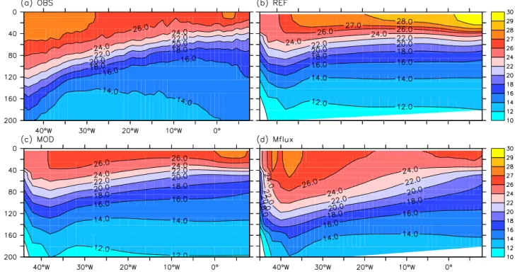
Figure 1 shows the long-term annual mean rainfall in the Tropical Atlantic from observation and the different experiments. The reference run simulates a wetter climate than observed in the east, and drier one in the west. Associated with the bias in rainfall, the zonal wind stress in REF displays much weaker easterly stress in the western to central Equatorial Atlantic compared to the ERA Interim reanalysis, and in the east, unrealistic westerly stress (the westerly bias) is simulated (Figure 2b). The westerly bias even exists in atmospheric GCMs (AGCM) with observed SST prescribed and has been attributed to erroneously weak diabatic heating in the western Equatorial Atlantic [Richter and Xie, 2008] and insufficient zonal momentum flux across the top of the boundary layer [Zerme~no-Diaz and Zhang, 2013;Richter et al., 2014b]. Correspondingly, REF shows much too warm SST in the eastern Equatorial Atlantic (Figure 2a) and the east-west SST gradient is reversed compared to observations. This bias is common to basically all state-of-the-art CGCMs [e.g., Richter and Xie, 2008;Richter et al., 2014a;Wang et al., 2014]. The thermocline in REF is too flat (Figure 3b) compared to the observed shoaling of the thermocline toward the east; this is consistent with the westerly wind bias (Figure 3a). The 20C isotherm (Z20) is situated in the middle of the highly stratified upper thermocline; for this reason this isotherm is used to measure the thermocline depth in this study, as in many other studies [e.g.,Keenlyside and Latif, 2007;Richter and Xie, 2008;Wahl et al., 2009].

In MOD, the computation of turbulent fluxes differs from REF as follows. In ECHAM5, the turbulent flux of a variableXis calculated according to the bulk transfer relation2CXjVLjðXL2XSÞ[Roeckner et al., 2003]. Here,X represents heat (h) or moisture (q), andCXis the transfer coefficient. The subscriptLandSdenote the lowest level in the atmospheric model and the surface level in the ocean model, respectively, andjVLjis surface wind speed. The transfer coefficient for heat and moisture can be expressed asCh5CNfhandCq5CNfq, respectively. Here,CNis the neutral transfer coefficient andfh(fq) is the stability function representing the ratio ofCh(Cq) to the value under neutral condition. The functionsfhandfqdepend on surface roughness (for instance land, ice, and sea) and atmospheric stability. For unstable conditions above sea surface, the stability function is given asf5ð11C^1:25_R Þ^1:25¹ whereCR5b^ðDH^v^Þ

1=3

CNjVLj. Here,Hvdenotes the virtual potential temperature difference between atmosphere and ocean at sea surface. In MOD, the parameterbinCRis increased in order to increase the transfer coefﬁcient of heat and moisture at sea surface for low wind speeds and large instabilities. The reader is referred toWahl et al. [2009] for more details on MOD.

Figure 1.Climatological mean state of precipitation is shown for (a) observations [Xie and Arkin, 1997] (b) REF run (c) MOD run, and (d) Mﬂux run. The unit is mm/day.

Journal of Geophysical Research: Oceans

10.1002/2014JC010384

(4)

The modiﬁcations in the turbulent transfer of heat and moisture at the ocean surface in MOD increase and reduce rainfall in the west and east, respectively, and thus lead to a better simulation of annual mean precipitation (Figure 1c). There are also striking differences in the mean zonal wind stress (Figure 2b) and SST (Figure 2a) between MOD and REF. MOD is about 2C (1C) colder with respect to REF (Figure 2a) in the eastern (western) Equatorial Atlantic, showing a ﬂat east-west SST structure. The westward wind stress at the equator (Figure 2b) is correspondingly enhanced in MOD compared with REF. Consistent with the enhanced zonal wind stress, upper ocean temperatures are improved (Figure 3c), amplifying the east-west tilt in the thermocline (Figures 2c and 3c).

Previous studies [Richter and Xie, 2008;Wahl et al., 2009] have shown that errors in the seasonal cycle of surface winds in the Equatorial Atlantic are the major source of error in SST there. Therefore, the third experiment (Mflux) employs flux correction in both zonal and meridional wind stress in the Tropical Atlantic between 10S and 10N. In this experiment, the climatological mean seasonal cycle of wind stress from the reference run (REF) is subtracted from the wind stress to obtain anomalous wind stress, which is transferred from atmospheric model to oceanic model. And then, the anomalous wind stress is added to NCEP/NCAR [Kalnay et al., 1996] monthly climatological wind stress and used to drive the ocean model. The flux correction in wind stress, by definition, strongly reduces the error in the mean seasonal cycle of the Equatorial Atlantic wind stress field, but still allows for coupled feedbacks and thus interannual variability. As a result, the SST warm bias is substantially reduced, so that the mean SST is very close to that observed (Figure 2a).

As a result, the precipitation pattern is also closer to observed with one pronounced rain band over the Atlantic to the North of the equator (Figure 1d). The mean thermocline depth in Mﬂux is considerably

Figure 2.Climatological mean state of (a) sea surface temperature, (b) zonal wind stress, and (c) thermocline depth calculated from observations and model experiments. In Figure 2a, observed reconstructed SST [Rayner et al., 2003] is shown. In Figure 2b, zonal wind stress from ERA Interim [Dee et al., 2011] and NCEP reanalysis [Kalnay et al., 1996] are shown. In Figure 2c, thermocline depth calculated from the World Ocean Atlas 2005 (WOA05;Locarnini et al. [2006]) is plotted. The units in Figures 2a, 2b, and 2c are Celsius, 10²²Pa andm, respectively.

Journal of Geophysical Research: Oceans

10.1002/2014JC010384

(5)

deeper than observed (Figure 2c) and the thermocline is too diffuse as in all the model configurations (Fig- ure 3). Note the momentum flux correction has a fixed seasonal cycle and does not depend on the model state. The improvement seen in Mflux is attributed to indirect effect of the momentum flux correction, which reduces the warm bias.

Apart from the errors in wind stress, there are other sources for the Tropical Atlantic SST bias. In particular, in the southeast, Tropical Atlantic SST bias has been attributed to excessive shortwave radiation at the surface [Huang et al., 2007;Hu et al., 2008], underestimation of coastal upwelling [Large and Danabasoglu, 2006], and low entrainment efficiency into the mixed layer [Hazeleger and Haarsma, 2005]. The formation of spurious barrier layers is shown to prevent surface cooling through strong salinity stratification and a subsurface temperature maximum, and may be responsible for a significant part of the eastern and southeastern Tropical Atlantic SST warm bias [Breugem et al., 2008].Haarsma et al. [2011] show that interruption of the Agulhas leakage can impact the simulation of mean state and interannual variability in the Tropical Atlantic. In addition, the KCM is a low-resolution model and cannot resolve lateral eddy fluxes which have been shown to be important for mean state and variability in the Tropical Atlantic [Jochum et al., 2004, 2005]. Recently,Wang et al. [2014] show that biases in special regions can be linked with other bias at far away locations so that it may not suffice to take only into account local effects for gaining an overall better model performance. Therefore, it is unlikely to achieve a realistic simulation of Tropical Atlantic variability in all regions by correcting only the momentum flux in the Equatorial Atlantic, even though the SST bias there is greatly reduced.

3. Results

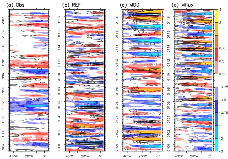
Figure 4 shows the SST and surface zonal wind anomalies along the Equatorial Atlantic for 20 year periods from observations during 1986–2005 and the three experiments. The observed SST anomalies are located in the central to eastern Atlantic, while surface zonal wind anomalies are located mostly in the west (Figure 4a), as revealed by previous studies [e.g.,Zebiak, 1993;Keenlyside and Latif, 2007]. The preferred locations for SST and surface zonal wind anomalies are further conﬁrmed through their standard deviations along the equator (see section 3.3). In REF, SST anomalies (Figure 4b) are located mainly in the western to central Atlantic. The relative position of SST and surface zonal wind anomalies in REF is less clear than in the

Figure 3.Climatological mean state of ocean temperature at the equator is shown for (a) observations (WOA05;Locarnini et al. [2006]) (b) REF run (c) MOD run, and (d) Mﬂux run. The unit isC.

Journal of Geophysical Research: Oceans

10.1002/2014JC010384

(6)

observations. In MOD (Figure 4c), the relative position of SST and surface zonal wind anomalies becomes clearer than in REF. We note that SST anomalies tend to occur in the east as in the observations, but surface zonal wind variability is still located in the middle of the basin. The best zonal structures of SST and surface zonal wind variability are seen in Mflux (Figure 4d), in which SST anomalies in the east are often accompa- nied by surface zonal wind stress anomalies in the west, indicating that they are coupled in a similar way as in observations (Figure 4a;Keenlyside and Latif[2007]). The major discrepancy to observations in Mflux and to a less extent MOD is that they simulate much too strong variability. In addition, the frequency of the variability seems higher in MOD and Mflux, but the mechanisms for this remain to be clarified.

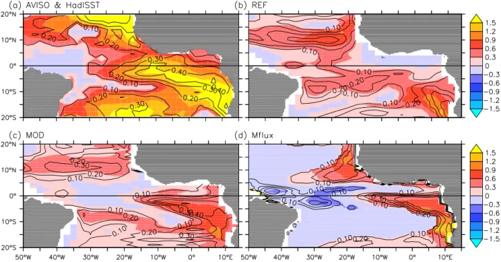
FollowingMu~noz et al. [2012] andLiu et al. [2013], we perform REOF analysis of Tropical Atlantic monthly mean (using all months) SST anomalies from 20S to 20N to extract the ZMs (Figure 5). Here, we use a nar- rower region than that (30S to 30N) used inMu~noz et al. [2012] andLiu et al. [2013] for analysis because we focus on variability at and near the equator. In observations, the first mode accounting for 26.4% of the variance corresponds to the ZM featuring maximum SST anomalies on the equator (Figure 5a). The second and third modes describe northern Tropical Atlantic mode (NTA; not shown) and subtropical South Atlantic mode (SSA; not shown) explaining 23.5% and 13.4% of the variance, respectively. We will discuss only the ZM (REOF1) in the following, since it is the main focus of this study. The ZM is captured by the third mode in REF accounting for 14.2% of the variance (Figure 5b), which is not surprising given that some CMIP5 models can also capture it [Mu~noz et al., 2012;Liu et al., 2013;Richter et al., 2014a]. In REF, it is expected that the ZM is not the first mode and explains less variance than in observations given maximum SST variability is seen in the western to central Equatorial Atlantic (Figure 4b) whereas the ZM describes SST variability in the eastern Equatorial Atlantic (Figure 5b). In contrast to REF, both MOD and Mflux capture the ZM as the first modes with explained variances of 29.4% and 35%, respectively. The higher explained variance in Mflux

Figure 4.Anomalies of SST (shading) and surface zonal winds (contours) at the equator in the Atlantic for periods of 20 years from (a) observations, (b) REF run, (c) Mod run, and (d) Mﬂux run. The interval of contours of surface zonal winds anomalies is 0:5 ms²¹. The unit of SST anomalies is Celsius. In Figure 4a, observed reconstructed SST [Rayner et al., 2003] and surface winds of ERA Interim [Dee et al., 2011] are plotted.

Journal of Geophysical Research: Oceans

10.1002/2014JC010384

(7)

compared with REF and MOD may be associated with the stronger Bjerknes feedback, as will be discussed next.

3.1. Bjerknes Feedback

The Bjerknes feedback loop consists of three elements: forcing of surface winds in the west by SST anomalies in the east, forcing of subsurface temperature anomalies in the east by winds to the west, and the forcing of SST anomalies in the east by subsurface temperature anomalies there. Previous studies have established the existence of the Bjerknes positive feedback loop in the Equatorial Atlantic [e.g.,Zebiak, 1993;Ruiz-Barradas et al., 2000;Keenlyside and Latif, 2007]. In this section, the three elements are investigated in the three KCM experiments and compared to those in observations.

The first element of the Bjerknes feedback is assessed by regressing surface zonal wind stress anomalies onto SST anomalies averaged over the Atl3 region (20W-0, 3S-3N). In the observations, zonal wind anomalies are to the west of the eastern Equatorial Atlantic SST anomalies, and only weak easterly anomalies are seen in the east (Figure 6a). The relation of zonal wind stress anomalies in the west to SST anomalies in the east is much weaker in REF (Figure 6b) than that in the ERA Interim reanalysis (Figure 6a). There are also unrealistically strong easterly wind stress anomalies in the central to eastern Atlantic (Figure 6b). These contribute to weaken the unrealistic westerly winds (Figure 2b), reducing heat flux and turbulent mixing and thus warming the ocean (see below). The link is somewhat improved in MOD (Figure 6c) compared with that in REF (Figure 6b) and comparable to that obtained from data (Figure 6a). However, the area with westerly wind stress anomalies (Figure 6c) corresponding to positive SST anomalies in the east is not con- fined to the west, but also extends northeastward to Africa and covers the Atl3 region. Therefore, the relative position of SST and surface zonal wind anomalies in MOD (Figure 4c) is improved compared to REF (Figure 4b), but is still less clear than in the observations (Figure 4a). In Mflux (Figure 6d), zonal wind stress in the west is related to SST variability in the east, but the relation is stronger than in the ERA Interim and other experiments: a 1C change in SST corresponds to maximum wind stress anomalies of above 0:01 Nm²²; while in the ERA Interim and MOD, this value is about 0:00820:01 Nm²²and

0:00620:008 Nm²², respectively. Furthermore, the local explained variance in Mﬂux is around 30–40%, which is higher than the 20–30% in observations, the 5–10% in REF, and the 20–30% in MOD. In summary, the three experiments exhibit rather different relationships between zonal wind stress and SST anomalies in the Equatorial Atlantic, consistent with a strong sensitivity of the interannual variability to the mean state, and all three simulations depict noticeable differences to the observed relationship.

Figure 5.Rotated EOF mode of SST anomalies in the Tropical Atlantic calculated from (a) observations [Rayner et al., 2003] (b) REF run (c) MOD run, and (d) Mﬂux run. Here, only Zonal- mode like REOF modes are shown. Explained variances are shown in brackets. See text for details.

Journal of Geophysical Research: Oceans

10.1002/2014JC010384

(8)

The Atlantic intertropical convergence zone (ITCZ) (Figure 1), where the northeast and southeast trade wind systems converge, is intimately coupled with SST in the eastern Equatorial Atlantic, and the meridional excursion of the ITCZ impacts surface zonal winds at the equator [e.g.,Xie and Carton, 2004;Richter et al., 2014a]. We note that the response of zonal wind stress to SST variability in the east (Figure 6) seems to be linked with the mean position of the Atlantic ITCZ (Figure 1). In the observations, the ITCZ covers the western Equatorial Atlantic and extends northeastward to Africa. Thus, zonal wind stress response to SST variability in the east is mainly located in the west (Figure 6a). In REF, the mean rainfall is located to the east of the Atl3 region, but very weak to the west (Figure 1b). Accordingly, zonal wind stress response is very weak in the west, and an unrealistic easterly anomalies is seen in the east (Figure 6b). The mean position of the ITCZ is improved in MOD compared with REF. In MOD (Figure 1c), the main rainfall belt is seen to the west of the Atl3 region, but still covers the central part of the Equatorial Atlantic between 40W and 10W; consis- tently, the zonal wind stress anomalies associated with Atl3 SST variability occur in the east (Figure 6c). The mean position of the ITCZ in Mﬂux (Figure 1d) is quite similar to that in the observations, and thus the pattern of zonal wind stress related to Atl3 SST is also similar to that in the observations, despite being too strong (Figure 6).

The second element of the Bjerknes feedback is estimated by regressing Z20 anomalies onto surface zonal wind stress anomalies averaged over the western Equatorial Atlantic (Watl, 40W-20W, 3S-3N) (Figure 7;

Keenlyside and Latif[2007]). Here, observed sea surface height (SSH) variations are employed as a proxy of Z20 variations, whereas thermocline depth is used from the models. The 20C isotherm (Z20) is situated in the middle of thermocline (Figure 3) and this makes it a measure of thermocline depth. In the equatorial oceans, SSH is closely related to Z20 [e.g.,Cane, 1984]. In fact, SSH is highly correlated with Z20 (up to 0.9) in the Equatorial Atlantic and a change in SSH of 1 cm is equivalent to a change of approximately 3 m in Z20 [Bunge and Clarke, 2009]. Western Equatorial Atlantic zonal wind stress anomalies are associated with an increase (decrease) in SSH in the east (west), particularly at (off) the equator (Figure 7a), indicating the effects of equatorial waves [Zebiak, 1993;Illig et al., 2004;Ding et al., 2009]. The regression patterns in the three KCM experiments (Figures 7b, 7c and 7d) closely resemble each other and that of observations (Figure 7a). This indicates that the second element of the Bjerknes feedback exists in the models. This result is expected, as the effect of model bias hardly affects equatorial shallow water dynamics, which is to

Figure 6.Regression (shading) of zonal wind stress anomalies onto the SST anomalies averaged over the Atl3 region (20W-0, 3S-3N) calculated from (a) observations, (b) REF run, (c) MOD run, and (d) Mﬂux run. The contours are the explained variances and the values of 0:05;0:1;0:2;0:3, and 0.4 are shown. The unit of regression coefﬁcients is Nm²²C²¹. In Figure 6a, observed reconstructed SST [Rayner et al., 2003] and ERA Interim [Dee et al., 2011] are plotted.

Journal of Geophysical Research: Oceans

10.1002/2014JC010384

(9)

first-order linear. Despite similarities in pattern, regression values and explained variances differ among the three KCM experiments. In REF, a 0:01 Pa anomaly over the WAtl region corresponds to a 224 m increase in thermocline depth with explained variances of about 20% in the east; in MOD and Mflux, these values are 628m and 40%, respectively. In the observations, the regression values are 1:221:6 cm for a 0:01 Pa anomaly in zonal wind stress, which corresponds 3:624:8 m [Bunge and Clarke, 2009]; the explained variances amount to about 20%. The higher explained variances in MOD and Mflux is consistent with the too strong ZMs simulated in the two experiments. The high regression values and explained variances may be associated with errors in the vertical ocean stratification (Figure 3), which impacts equatorial wave dynamics, and the pattern of zonal wind stress. Understanding the sensitivity of the second element to ocean stratification is beyond the scope of the current study.

The last element of the Bjerknes feedback is estimated by regressing SST anomalies onto local Z20 anomalies (Figure 8;Keenlyside and Latif[2007]). In the eastern Equatorial Atlantic, SSH and SST variability are tightly coupled (Figure 8a); SSH is again used as a proxy for Z20 [e.g.,Cane, 1984]. Regression values show that a 10 cm rise in SSH corresponds to a warming of 1:2C in SST with an explained variance of about 30%–40% (Figure 8a). In terms of the relationship between SSH and Z20 in the Equatorial Atlantic [Bunge and Clarke, 2009], this is equivalent to a warming of 0:4C in SST in association with a deepening of 10 m in Z20. In contrast to the observations, subsurface and surface variability at the equator in REF is only weakly coupled in the east (Figure 8b). This is consistent with the climatological mean surface winds being biased westerly to the east of 20W that implies Ekman downwelling rather than upwelling according to equation (9.4.2) inGill[1982], as explained further in section 3.3. Therefore, mean downwelling cannot advect subsurface temperature anomalies upward to impact SST variability in the east. To some extent both MOD (Figure 8c) and Mﬂux (Figure 8d), capture the observed relation between subsurface temperature and SST variability in the east. In MOD and Mﬂux, a 10 m increase in Z20 depth corresponds to a warming of SST about 0:320:4C, and explained variances are in the range of 30–40%.

Regression analysis using observations (Figure 8a) also shows that surface and subsurface temperature variations are coupled along the African coast, in particular between 10S and 20S. SST variability there is also important for climate [e.g.,Rouault et al., 2003;Huang et al., 2004;Hu and Huang, 2007]. Many Benguela

Figure 7.The regression (shading) of SSH/Z20 anomalies onto wind stress anomalies averaged over western equatorial Atlantic (Watl, 40W-20W, 3S-3N) calculated from (a) observations, (b) REF run, (c) MOD run, and (d) Mﬂux run. The contours are the explained variances and their interval is 0.1. In Figure 7a, zonal wind stress is from ERA Interim [Dee et al., 2011]

and sea surface height from satellite is used as an agent for thermocline depth. In Figures 7b–7d, thermocline depth is used for subsurface. The unit of the regression coefﬁcients in Fig- ures 7a and 7b–7d are cmN²¹m²and mN²¹m², respectively.

Journal of Geophysical Research: Oceans

10.1002/2014JC010384

(10)

Ni~no’s are associated with the relaxation of the trade winds in the western Equatorial Atlantic; the relaxation excites equatorial Kelvin waves that propagate to the African coast and then down to the Benguela Ni~no upwelling region [e.g.,Florenchie et al., 2004;Hu and Huang, 2007;L€ubbecke et al., 2010]. Local physical pro- cess may also explain some Bengula Ni~no events [Richter et al., 2010]. In contrast to distinct performance at the equator, all the model experiments capture to some extent the subsurface and surface coupling in the southeast Atlantic. Detailed analysis of simulation of interannual variability along the African coast is beyond the scope of this study, which focuses on Equatorial Atlantic variability.

In summary, the three elements of the Bjerknes feedback exist to some degree in all the three experiments.

In the REF, the first and third elements are much weaker than those in MOD and Mflux, consistent with less variance of the ZM in REF. In Mflux, the first element of the Bjerknes feedback is slightly stronger than observed, and much stronger than in MOD. In MOD and Mflux, the second and third elements of the Bjerknes feedback resembles each other. The stronger Bjerknes feedback in Mflux than in MOD is consistent with the ZM greater explained in Mflux.

3.2. Delayed Negative Feedback

A delayed negative feedback is necessary for an oscillatory behavior, as has been documented for the El Ni~no Southern Oscillation in the Equatorial Pacific [Zebiak and Cane, 1987;Jin, 1997]. In the Equatorial Atlantic, previous studies showed that the delayed negative feedback is also an important element of the interannual variability in intermediate coupled [Zebiak, 1993], conceptual [Jansen et al., 2009], and theoretical [Wang and Chang, 2008] models and observations [Ding et al., 2010]. For instance,Ding et al. [2010] document the build-up of heat content in the Equatorial Atlantic prior to the mature phase of the ZM from both observations and a forced ocean model integration (Figure 9a), and show the net surface heat flux acts mainly to damp SST anomalies in the eastern Equatorial Atlantic (Figure 9b;Hu and Huang[2006, 2007]). In this section, we explore the roles of upper ocean heat content and net surface heat flux in the interannual variability of the Equatorial Atlantic in the three KCM experiments and also depict the links from observations and the ORA-S4 ocean reanalysis.

In REF, the cross correlation between equatorial heat content and eastern equatorial SST anomalies (Figure 9a) is always negative, indicating that there is no build-up of heat content prior to warm SST anomalies and

Figure 8.The regression (shading) of sea surface temperature anomalies onto local SSH/Z20 anomalies calculated from (a) observations, (b) REF run, (c) MOD run, and (d) Mﬂux run. The contours are the explained variances and their interval is 0.1. In Figure 8a, observed reconstructed SST [Rayner et al., 2003] is employed and sea surface height from satellite is used as a measure of subsurface variability. In Figures 8b–8d, thermocline depth is used as a measure of subsurface variability. The units of the regression coefﬁcients in Figures 8a and 8b–8d are Ccm²¹and Cm²¹, respectively.

Journal of Geophysical Research: Oceans

10.1002/2014JC010384

(11)

vice versa. This is not surprising consid- ering that the thermocline is only weakly coupled to local SST variability (Figure 8b). To shed light on the mechanism for SST variability in the east in this experiment, the relationship between net surface heat ﬂux and SST is further analyzed; their cross correlation (Figure 9b) displays a positive (negative) peak when the former leads (lags) the latter by 2 (two) months, indicating that net surface heat ﬂux anomalies drive SST anomalies in REF.

The heat ﬂux forcing is consistent with the weakening of the unrealistic westerly winds by easterly wind anomalies (Figures 2b and 6b).

In MOD, there is clear link between heat content in the equatorial wave guide and eastern equatorial SST anomalies that can be inferred from the maximum positive correlation when heat content leads SST by 2 months (Figure 9a). This phase relationship is in accord with the delayed action/recharge oscillator mechanism [Jin, 1997]. Principal oscillation pattern (POP) analysis of monthly Z20, SST, and wind stress reveals one dominant POP mode (not shown) that is consistent with results presented here, and further supports the delayed action/

recharge oscillator mechanism in MOD.

The role of ocean dynamics in driving SST variability is further supported by the simultaneous anticorrelation between net surface heat flux and SST anomalies in the east (Figure 9b). In Mflux, the phase relationship between equatorial upper ocean heat content and SST averaged over Atl3 region (Figure 9a) is also consistent with the delayed action/recharge oscillator mechanism. But the link between the prior build-up of heat content and SST in Mflux is weaker than that in MOD. On the other hand, the delayed negative feedback is stronger in Mflux (r5 20.5) than in MOD (r5 20.4). Consistent with ocean dynamics driving SST variability, the net surface heat flux acts mainly to damp the cold eastern equatorial SST anomalies (Figure 9b).

3.3. Seasonality of Equatorial Atlantic Variability

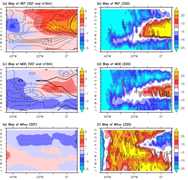
We now investigate the seasonality of Equatorial Atlantic variability in the simulations, beginning with SST, surface zonal wind, and Z20 biases at the equator (Figure 10). In REF (Figure 10), a strong westerly wind bias appears during boreal spring (MAM) that extends almost across the entire Equatorial Atlantic. The westerly wind bias induces deeper thermocline than observed in the east. The positive Z20 bias peaks in May and June, with maximum positive bias of more than 25 m. The bias is so large in May and June that the seasonal cycle of Z20 in the east is almost opposite to that in the observations (Figures 11a and 11b). The unrealistically deep thermocline in the east inhibits upwelling of cold water, causing the maximum warm SST bias during boreal summer (JJA). The seasonal evolution of the bias in REF is consistent with that inRichter and Xie[2008], as described inWahl et al. [2009].

Figure 9.The cross correlation between (a) SSH/Z20 averaged over the Equatorial Atlantic and SST anomalies averaged over Atl3 region and (b) net surface heat ﬂux anomalies and SST anomalies averaged over Atl3 region. In Figure 9a, ORA-S4 denotes 20C isotherm depths, a measure of subsurface variability, from ECMWF Ocean Reanalysis System 4 (ORAS4;Balmaseda et al. [2013]) and AVISO denotes satellite measurement of SSH (http://www.aviso.oceanobs.com/). In Figure 9b, OBS denotes cross correlation between net surface heat ﬂux [Kalnay et al., 1996] and observed reconstructed SST [Rayner et al., 2003].

Journal of Geophysical Research: Oceans

10.1002/2014JC010384

(12)

While the biases in MOD are somewhat reduced compared with REF, they exhibit similar seasonal evolution:

there is a maximum westerly wind bias from April to June in the west, a maximum positive Z20 bias in May and June in the east, and the largest SST bias from June to August in the east (Figures 10c and 10d). The seasonal cycle of Z20 is still almost opposite to that in observations (Figures 11a and 11c). In particular, thermocline shoaling in the east occurs in August–September in MOD, but in June–July in the observations. The lag of about 2 months (compared with observations) in the thermocline shoaling in the east may cause some phase lag in the Bjerknes feedback and thus SST variability between MOD and observations, as discussed below.

In Mflux, the seasonal cycle of both zonal and meridional wind stress from the NCEP reanalysis (see Figure 2b for zonal wind stress) is employed via momentum flux correction. The deeper Z20 bias in the east seen in May and June in both REF and MOD is largely reduced (Figures 10e and 10f), because of the more realistic surface zonal wind stress. Correspondingly, the warm SST bias from June to August seen in both REF and MOD is also largely reduced in the east. In general, Mflux displays the best phase of the seasonal cycle of Z20 of all the simulations, with shallower thermocline from June to September in the east (Figures 11a and 11d). Nevertheless, the simulated seasonal cycle of Z20 is stronger than observed and some moderate SST errors remain.

Figure 10.Longitude-time sections of biases of surface zonal winds (contours shown in left), SST (shading shown in left side) and Z20 (right side) at the equator (averaged between 2S and 2N) calculated from (a and b) REF, (c and d) MOD, and (e and f) Mﬂux experiments. The units of surface zonal winds, SST, and Z20 are ms²¹, Celsius, and m, respectively.

Journal of Geophysical Research: Oceans

10.1002/2014JC010384

(13)

Monthly stratified standard deviations of SST at the equator shows there are also marked differences in the seasonality of SST variability among the simulations and observations (Figure 12). In observations, the maximum SST variability is in the east from June to July (Figure 12a), as has been reported by many previous studies [e.g.,Xie and Carton, 2004;Keenlyside and Latif, 2007;Richter et al., 2014a]. The observations show a second peak in SST variability in November and December that has been referred to as the second Atlantic Ni~no [Okumura and Xie, 2006]. In REF, SST variability peaks around May, but the maximum is found in the central Atlantic to the west of the observed maximum (Figures 12a and 12b); as was noted from the Hov- moeller diagrams of equatorial SST anomalies (Figures 4a and 4b). In MOD and Mflux, SST variability is located mainly in the eastern part of the Equatorial Atlantic (see also Figures 4c and 4d), and is more consistent with observations than REF. However, MOD simulates maximum SST variability from July to Septem- ber, about 2 months later than that in the observations and Mflux. This may be associated with the delayed seasonal cycle of Z20 (Figure 11c). Mflux has the best simulation in terms of phase, capturing the maximum SST variability in June and July. A notable deficiency of MOD and Mflux is that they simulate stronger SST variability than observed: the maximum SST variability in MOD is 0:821C and in Mflux is 1:221:5C, while the observed is 0:620:7C.

We further investigate if seasonal variations of the Bjerknes feedback is able to explain the seasonality of observed and simulated variability [Keenlyside and Latif, 2007]. Figure 13 shows monthly stratiﬁed correlations of SST anomalies averaged over the eastern Equatorial Atlantic (Atl3 region) with zonal wind stress and monthly stratiﬁed pointwise correlations between SST and SSH/Z20 anomalies along the equator. The observations (Figure 13a) depict that zonal wind stress and SST anomalies are most strongly related during

Figure 11.Longitude-time sections of seasonal cycle of Z20 at the equator (averaged between 2S and 2N) calculated from (a) WOA05 observations [Locarnini et al., 2006] and (b) REF, (c) MOD, and (d) Mﬂux experiments. The unit of Z20 is m.

Journal of Geophysical Research: Oceans

10.1002/2014JC010384

(14)

late spring and early summer (April–June), and the link between the subsurface and surface is strongest from May to July. The seasonality of these two components of the Bjerknes feedback explains the phase locking of ZM to boreal summer [Keenlyside and Latif, 2007]. The two components of the Bjerknes feedback strengthen in November and December (Figure 13a), which has been shown to be associated with the second Atlantic Ni~no [Okumura and Xie, 2006].

In REF (Figure 13b), zonal wind stress and SST anomalies are also related, but the correlations are weaker than observed. The strongest relation is in May, it weakens in summer, but strengthens again from October to December. There is an apparent subsurface temperature signal between 40W and 10W around May when the thermocline is shallower (Figure 11b) and related to local SST variations (Figure 8b). Eastern Atlantic SST variations are also related to subsurface temperature to the east of 10W from November to the next February when the thermocline is again closer to the surface. The seasonality of these two components of the Bjerknes feedback components is consistent with the enhanced SST variability at the equator in May, December, and January (Figure 12b). It is not consistent with the enhanced SST variability later in the summer.

In MOD (Figure 13c), the strongest link between zonal wind stress and SST anomalies is seen from June to December. The relation between eastern Equatorial Atlantic SST and subsurface temperature is strongest from July to September in the east (Figure 13c) when the thermocline is shallower (Figure 11c). The link between subsurface and surface variability is also seen from December to the next March (Figure 13c) when the thermocline is relatively shallow (Figure 11c). The seasonality of these Bjerknes feedback components is consistent with the seasonality of SST variability at the equator (Figure 12c). In particular, both the

Figure 12.Longitude-time sections of monthly stratiﬁed standard deviation of SST along the equator (averaged between 2S and 2N) calculated from (a) observation [Rayner et al., 2003], (b) REF run, (c) MOD run, and (d) Mﬂux run. The unit is Celsius.

Journal of Geophysical Research: Oceans

10.1002/2014JC010384

(15)

maximum SST variability (Figure 12c) and shallowest thermocline (Figure 11c) occur during July–September, about 2 months later than that in the observations (Figures 12a and 11a).

In Mflux (Figure 13d), zonal wind stress and SST anomalies are strongly related from April to July. In addition, the link between subsurface and surface is strongest from May to July in the east (Figure 13c) a period during which the climatological thermocline becomes shallower (Figure 11d). The relation between these two components of the Bjerknes feedback is more consistent with those in observations compared with REF and MOD (Figure 13). The more realistic seasonality of the Bjerknes feedback components is in agreement with the better seasonality of SST variability in Mflux than that in REF (Figure 12b) and MOD (Figure 12c). Although the spatial pattern of SST variability in Mflux (Figures 4d and 12d) resembles that in MOD (Figures 4c and 12c), the seasonality in Mflux (Figure 12d) is improved compared to MOD (Figure 12c). The improvement is likely because the seasonal variations of the Bjerknes feedback in Mflux (Figure 13d) is more consistent with that in observations than in MOD (Figure 13c). This in turn seems tied to primarily to the seasonal cycle of subsurface variability and the development of the cold tongue.

4. Summary and Discussion

This work was motivated by two questions: Can simulation of interannual variability be improved in a CGCM if the bias is reduced? What is the inﬂuence of the warm bias on the mechanism of Atlantic Ni~no? To

Figure 13.Longitude-time sections of monthly stratiﬁed correlation (contours) between zonal wind stress and SST anomalies averaged over the Atl3 region and point wise correlation (shading) between SSH/Z20 and SST anomalies calculated from (a) observation, (b) REF run, (c) MOD run, and (d) Mﬂux run. In Figure 13a, satellite-observed SSH (http://www.aviso.oceanobs.com/) and the ERA Interim reanalysis [Dee et al., 2011] are plotted.

Journal of Geophysical Research: Oceans

10.1002/2014JC010384

(16)

address these, we investigate the interannual variability in the Equatorial Atlantic in three experiments conducted with different formulations of the Kiel Climate Model (KCM,Park et al. [2009]) and thus different climatological states (Figure 2;Wahl et al. [2009]). In the run with the standard version of the KCM, termed REF, there is a large warm bias in SST in the eastern Tropical Atlantic (Figure 2a), whereas in a modified physics run, termed MOD, and especially in a run that employed zonal and meridional momentum flux correction, termed Mflux, the warm bias is greatly reduced (Figure 2a).

All three experiments simulate zonal mode (ZM) like variability with an SST pattern similar to that in observations, but with different explained variances (Figure 5). In REF, the ZM explains 14.2% of Tropical Atlantic SST variance, and this is only half of that in observations (26.4%). The explained variance of ZM increases to 29.4% in MOD, and to almost 35% in Mﬂux. The higher variance of the ZM is associated with the more realistic mechanisms for Equatorial Atlantic variability in MOD and Mﬂux.

Analysis of the three components of the Bjerknes feedback shows that they are all more realistic in MOD and Mflux than in REF, and that the differences can be related to the different mean states. First, an erroneous relation with easterly wind anomalies over the warm eastern Atlantic SST is simulated in REF. This appears related to the erroneous climatological precipitation and westerly winds overly an eastern Atlantic warm pool. In this configuration, an anomalous increase in precipitation leads to anomalous easterlies in the east, and thus to reduced surface heat flux cooling and upper ocean entrainment, and in turn warming of SST. In MOD and Mflux, climatological precipitation patterns are close to observed, and thus the relation between wind stress and eastern Atlantic SST resembles observations, with westerly wind anomalies to the west of warm SST anomalies. Second, in REF, there is a weak link between subsurface temperature and SST variability in the west. While in observations, MOD, and Mflux, the link is found in the east (Figure 8). In addition, the delayed negative feedback in MOD and Mflux operates in a manner consistent with observations.

But in REF, the delayed negative feedback is not found. Rather, net surface heat ﬂux leads and thus drives SST variability in the east. These differences appear related with the unrealistic climatological westerlies in REF that drive downwelling in the east, and the climatological easterlies in observations and the other models that drive upwelling (Figure 2). Furthermore, the missing of the delayed negative feedback could be the main reason that seasonal prediction is not skillful in the eastern Equatorial Atlantic in coupled models [Stockdale et al., 2006], which have large warm biases there. However, analysis of forecast experiments is needed to conﬁrm this.

The seasonality of the ZM-like variations was shown to differ among the three simulations, and these differences could also be related to the impact of mean state errors on the representation of ocean-atmosphere interaction. In particular, in REF SST variability at the equator peaks in May in the central Atlantic. The observed peak in SST anomalies further to the east and in June–August appears inhibited in REF by the erroneous seasonal cycle of thermocline depth and zonal winds: In observations in the east, the equatorial easterly zonal winds and upwelling are at their climatological strongest, and the thermocline shoals; while in REF the thermocline is at its climatological deepest, and the equatorial zonal winds in the east are westerly, driving downwelling. The seasonality of Equatorial Atlantic variability is not improved in MOD with respect to REF despite a more realistic ZM and the improved representation of the Bjerknes feedback and the delayed negative feedback. This is probably because there is still a strong bias in the simulation of the seasonal cycle in MOD. For instance, the westerly bias seen in the REF in April–May is only slightly reduced in MOD. As a result, the seasonal cycle of thermocline depth in MOD is still like that in REF, and nearly opposite to that in observations. This basically inhibits the development of an Equatorial Atlantic cold tongue.

The bias in the seasonal cycle changes the seasonality of the Bjerknes feedback, so that in REF SST variability peaks around May, while in MOD it peaks from July to September. In Mﬂux, the seasonal cycle of thermocline depth is closer to observations, as expected. As a result, the seasonality of the Bjerknes feedback is also more consistent with observations so that Mﬂux simulates maximum SST variability in June and July as observed. However, the feedback appears too strong and simulated variability is larger than observed; the model also misses the second Atlantic Ni~no.

In MOD and Mflux, the warm bias is greatly reduced with respect to REF (Figure 2a;Wahl et al. [2009]), but is achieved through different approaches: parameter tuning and momentum flux correction, respectively. The positive Bjerknes feedback and delayed negative feedback in these two experiments operate in a manner consistent with observations. As these feedbacks are linked to the mean state, it is plausible to assume that the more realistic simulation of Equatorial Atlantic interannual variability in MOD and Mflux is primarily

Journal of Geophysical Research: Oceans

10.1002/2014JC010384

(17)

achieved through the improved mean state. Furthermore, in Mﬂux, where momentum ﬂux correction is used, the changes in the feedbacks relative to those in REF can only result from changes in the mean state.

In MOD, they may result from both the changes in the mean state and the changes in the physical parameterization, where the latter has a direct influence on the dynamics of the coupled system. The two model configurations show (1) that the simulation of interannual variability remains deficient when the mean state is artificially corrected (Mflux); and (2) that moderate reductions of model mean error (MOD) will lead to substantial improvements in the simulation of interannual variability, although simulating its seasonality remains a challenge. Mflux is still deficient in many aspects. This is not surprising given that apart from wind stress, many other factors, which cannot be accounted for by momentum flux correction, contribute to SST bias in the Tropical Atlantic [e.g.,Huang et al., 2007;Hu et al., 2008;Large and Danabasoglu, 2006;

Hazeleger and Haarsma, 2005;Haarsma et al., 2011;Jochum et al., 2004, 2005;Breugem et al., 2008]. Further improvement through e.g., enhanced horizontal [e.g.,Jochum et al., 2004, 2005] and vertical resolution [e.g., Breugem et al., 2008], or the inclusion of remote effects [e.g.,Haarsma et al., 2011;Wang et al., 2014] is required. These aspects should be investigated in future studies.

In this study, we have focused on the positive Bjerknes and delayed negative feedback. However, these two mechanisms explain much less variance in the Equatorial Atlantic than in the Equatorial Pacific [Keenlyside and Latif, 2007;Ding et al., 2010]. Some other dynamics may also contribute to Equatorial Atlantic interannual variability. In particular, complex remote forcing from ENSO [e.g.,Chang et al., 2006] might contribute to mask the heat content signal remotely forced by the Equatorial Pacific through changes in the Walker Circulation. Other possible mechanisms include the western Pacific oscillator [Weisberg and Wang, 1997], the advective- reflective oscillator [Picaut et al., 1997;Wang, 2001], destabilized basin modes [Jin and Neelin, 1993;Keenlyside and Latif, 2007;Keenlyside et al., 2007], or a link between Equatorial and subtropical Atlantic [Richter et al., 2012], including with variations over the South Atlantic [L€ubbecke et al., 2010;Nnamchi et al., 2011]. Ocean dynamics may also be less important (H. Nnamchi, personal communication). Moreover, the meridional mode [e.g.,Xie and Carton, 2004], which contributes to decadal variability in the Tropical Atlantic, may also affect interannual variability. The investigation of these possible mechanisms is beyond the scope of this study.

In summary, the results of this study suggest that a better simulation of interannual variability in the Equa- torial Atlantic can be achieved through improving the mean state in coupled ocean-atmosphere general circulation models. This, however, is not trivial, because the climate system in the equatorial sector is strongly coupled, giving rise to a high sensitivity to errors in individual model components so that biases in different component models and regions could be linked with each other [Wang et al., 2014]. With respect to seasonal forecasting, momentum ﬂux correction could be an option, as long as the coupled models suffer from large biases. Nevertheless, as shown here momentum ﬂux correction cannot fully correct ocean-

atmosphere feedbacks.

References

Balmaseda, M. A., K. Mogensen, and A. T. Weaver (2013), Evaluation of the ECMWF ocean reanalysis system ORAS4,Q. J. R. Meteorol. Soc., 139(674), 1132–1161, doi:10.1002/qj.2063.

Battisti, D. S., and A. C. Hirst (1989), Interannual variability in a tropical atmosphere-ocean model: Inﬂuence of the basic state, ocean geom- etry and nonlinearity,J. Atmos. Sci.,46(12), 1687–1712, doi:10.1175/1520-0469(1989)046<1687:IVIATA>2.0.CO;2.

Blanke, B., and P. Delecluse (1993), Variability of the tropical Atlantic Ocean simulated by a general circulation model with two different mixed-layer physics,J. Phys. Oceanogr.,23(7), 1363–1388, doi:10.1175/1520-0485(1993)023<1363:VOTTAO>2.0.CO;2.

Bougeault, P., and P. Lacarrere (1989), Parameterization of orography-induced turbulence in a Mesobeta–scale model,Mon. Weather Rev., 117(8), 1872–1890, doi:10.1175/1520-0493(1989)117<1872:POOITI>2.0.CO;2.

Breugem, W.-P., P. Chang, C. Jang, J. Mignot, and W. Hazeleger (2008), Barrier layers and tropical Atlantic SST biases in coupled GCMs,Tellus Ser. A,60(5), 885–897, doi:10.1111/j.1600-0870.2008.00343.x.

Bunge, L., and A. Clarke (2009), Seasonal propagation of sea level along the equator in the Atlantic,J. Phys. Oceanogr.,39(4), 1069–1074, doi:10.1175/2008JPO4003.1.

Cane, M. A. (1984), Modeling sea level during El Ni~no,J. Phys. Oceanogr.,14(12), 1864–1874, doi:10.1175/1520-0485(1984)014<1864:

MSLDEN>2.0.CO;2.

Carton, J., and B. Huang (1994), Warm events in the tropical Atlantic,J. Phys. Oceanogr.,24(5), 888–903, doi:10.1175/1520-0485(1994)024

<0888:WEITTA>2.0.CO;2.

Chang, P., Y. Fang, R. Saravanan, L. Ji, and H. Seidel (2006), The cause of the fragile relationship between the Paciﬁc El Ni~no and the Atlantic Ni~no,Nature,443(7109), 324–328, doi:10.1038/nature05053.

Dee, D., et al. (2011), The ERA-Interim reanalysis: Conﬁguration and performance of the data assimilation system,Q. J. R. Meteorol. Soc., 137(656), 553–597, doi:10.1002/qj.828.

Ding, H., N. Keenlyside, and M. Latif (2009), Seasonal cycle in the upper equatorial Atlantic Ocean,J. Geophys. Res.,114, C09016, doi:

10.1029/2009JC005418.

Acknowledgments

This work was supported by the RACE and SACUS projects of the BMBF and GEOMAR, and the EU FP7 projects PREFACE (grant agreement 603521) and STEPS (PCIG10-GA-2011–304243).

Figures were created using Ferret, a product of NOAAs Paciﬁc Marine Environmental Laboratory. Data shown in this paper are available by email (hding@geomar.de) from corresponding author.

Journal of Geophysical Research: Oceans

10.1002/2014JC010384

(18)

Ding, H., N. Keenlyside, and M. Latif (2010), Equatorial Atlantic interannual variability: The role of heat content,J. Geophys. Res.,115, C09020, doi:10.1029/2010JC006304.

Ding, H., N. Keenlyside, and M. Latif (2011), Impact of the equatorial Atlantic on the El Ni~no southern oscillation,Clim. Dyn.,38(9–10), 1965–

1972, doi:10.1007/s00382-011-1097-y.

Ding, H., R. J. Greatbatch, M. Latif, W. Park, and R. Gerdes (2013), Hindcast of the 1976/77 and 1998/99 climate shifts in the Paciﬁc,J. Clim., 26(19), 7650–7661, doi:10.1175/JCLI-D-12-00626.1.

Ding, H., R. J. Greatbatch, W. Park, M. Latif, V. A. Semenov, and X. Sun (2014a), The variability of the East Asian summer monsoon and its relationship to ENSO in a partially coupled climate model,Clim. Dyn.,42(1-2), 367–379, doi:10.1007/s00382-012-1642-3.

Ding, H., R. J. Greatbatch, and G. Gollan (2014b), Tropical impact on the interannual variability and long-term trend of the Southern Annular Mode during austral summer from 1960/1961 to 2001/2002,Clim. Dyn.,1–14, doi:10.1007/s00382-014-2299-x.

Fedorov, A. V., and S. G. Philander (2001), A stability analysis of tropical ocean-atmosphere interactions: Bridging measurements and theory for El Nino,~ J. Clim.,14(14), 3086–3101, doi:10.1175/1520-0442(2001)014<3086:ASAOTO>2.0.CO;2.

Florenchie, P., C. Reason, J. Lutjeharms, M. Rouault, C. Roy, and S. Masson (2004), Evolution of interannual warm and cold events in the southeast Atlantic Ocean,J. Clim.,17(12), 2318–2334, doi:10.1175/1520-0442(2004)017<2318:EOIWAC>2.0.CO;2.

Folland, C., T. Palmer, and D. Parker (1986), Sahel rainfall and worldwide sea temperatures, 1901–85,Nature,320(6063), 602–607, doi:

10.1038/320602a0.

Frauen, C., and D. Dommenget (2012), Inﬂuences of the tropical Indian and Atlantic Oceans on the predictability of ENSO,Geophys. Res.

Lett.,39, L02706, doi:10.1029/2011GL050520.

Gaspar, P., Y. Gregoris, and J.-M. Lefevre (1990), A simple eddy kinetic energy model for simulations of the oceanic vertical mixing: Tests at station Papa and long-term upper ocean study site,J. Geophys. Res.,95(C9), 16,179–16,193, doi:10.1029/JC095iC09p16179.

Gill, A. (1982),Atmosphere-ocean dynamics, International Geophysics Series, vol. 30, 662 pp., Academic Press, London, U. K.

Guemas, V., F. J. Doblas-Reyes, I. Andreu-Burillo, and M. Asif (2013), Retrospective prediction of the global warming slowdown in the past decade,Nat. Clim. Change,3(7), 649–653, doi:10.1038/nclimate1863.

Haarsma, R. J., E. J. Campos, S. Drijfhout, W. Hazeleger, and C. Severijns (2011), Impacts of interruption of the Agulhas leakage on the tropical Atlantic in coupled ocean–atmosphere simulations,Clim. Dyn.,36(5-6), 989–1003, doi:10.1007/s00382-009-0692-7.

Hazeleger, W., and R. J. Haarsma (2005), Sensitivity of tropical Atlantic climate to mixing in a coupled ocean–atmosphere model,Clim. Dyn., 25(4), 387–399, doi:10.1007/s00382-005-0047-y.

Hazeleger, W., et al. (2012), EC-Earth V2. 2: Description and validation of a new seamless earth system prediction model,Clim. Dyn.,39(11), 2611–2629, doi:10.1007/s00382-011-1228-5.

Hu, Z., and B. Huang (2006), Physical processes associated with the tropical Atlantic SST meridional gradient,J. Clim.,19(21), 5500–5518, doi:10.1175/JCLI3923.1.

Hu, Z., and B. Huang (2007), Physical processes associated with the tropical Atlantic SST gradient during the anomalous evolution in the southeastern ocean,J. Clim.,20(14), 3366–3378, doi:10.1175/JCLI4189.1.

Hu, Z.-Z., B. Huang, and K. Pegion (2008), Low cloud errors over the southeastern Atlantic in the NCEP CFS and their association with lower-tropospheric stability and air-sea interaction,J. Geophys. Res.,113, D12114, doi:10.1029/2007JD009514.

Huang, B., P. S. Schopf, and J. Shukla (2004), Intrinsic ocean-atmosphere variability of the tropical Atlantic Ocean,J. Clim.,17(11), 2058–

2077, doi:10.1175/1520-0442(2004)017<2058:IOVOTT>2.0.CO;2.

Huang, B., Z.-Z. Hu, and B. Jha (2007), Evolution of model systematic errors in the tropical Atlantic basin from coupled climate hindcasts, Clim. Dyn.,28(7-8), 661–682, doi:10.1007/s00382-006-0223-8.

Illig, S., B. Dewitte, N. Ayoub, Y. du Penhoat, G. Reverdin, P. De Mey, F. Bonjean, and G. Lagerloef (2004), Interannual long equatorial waves in the tropical Atlantic from a high-resolution ocean general circulation model experiment in 1981–2000,J. Geophys. Res.,109, C02022, doi:10.1029/2003JC001771.

Jansen, M., D. Dommenget, and N. Keenlyside (2009), Tropical atmosphere–ocean interactions in a conceptual framework,J. Clim.,22(3), 550–567, doi:10.1175/2008JCLI2243.1.

Jin, F. (1997), An equatorial ocean recharge paradigm for ENSO. Part I: Conceptual model,J. Atmos. Sci.,54(7), 811–829, doi:10.1175/1520- 0469(1997)054<0811:AEORPF>2.0.CO;2.

Jin, F., and J. Neelin (1993), Modes of interannual tropical ocean-atmosphere interaction-a uniﬁed view. Part I: Numerical results,J. Atmos.

Sci.,50(21), 3477–3477, doi:10.1175/1520-0469(1993)050<3477:MOITOI>2.0.CO;2.

Jochum, M., P. Malanotte-Rizzoli, and A. Busalacchi (2004), Tropical instability waves in the Atlantic Ocean,Ocean Modell.,7(1), 145–163, doi:10.1016/S1463-5003(03)00042-8.

Jochum, M., R. Murtugudde, R. Ferrari, and P. Malanotte-Rizzoli (2005), The impact of horizontal resolution on the tropical heat budget in an Atlantic Ocean model,J. Clim.,18(6), 841–851, doi:10.1175/JCLI-3288.1.

Kalnay, E., et al. (1996), The NCEP/NCAR 40-year eeanalysis project,Bull. Am. Meteorol. Soc.,77(3), 437–471, doi:10.1175/1520- 0477(1996)077<0437:TNYRP>2.0.CO;2.

Keenlyside, N., and M. Latif (2007), Understanding equatorial Atlantic interannual variability,J. Clim.,20(1), 131–142, doi:10.1175/

JCLI3992.1.

Keenlyside, N., M. Latif, and A. Durkop (2007), On sub-ENSO variability,J. Clim.,20(14), 3452–3469, doi:10.1175/JCLI4199.1.

Keenlyside, N. S., H. Ding, and M. Latif (2013), Potential of equatorial Atlantic variability to enhance El Ni~no prediction,Geophys. Res. Lett., 40, 2278–2283, doi:10.1002/grl.50362.

Large, W., and G. Danabasoglu (2006), Attribution and impacts of upper-ocean biases in CCSM3,J. Clim.,19(11), 2325–2346, doi:10.1175/

JCLI3740.1.

Latif, M., W. Park, H. Ding, and N. Keenlyside (2009), Internal and external North Atlantic sector variability in the Kiel climate model,Mete- orol. Z.,18(4), 433–443, doi:10.1127/0941-2948/2009/0395.

Liu, H., C. Wang, S.-K. Lee, and D. Enﬁeld (2013), Atlantic warm pool variability in the CMIP5 simulations.,J. Clim.,26(15), 5315–5336, doi:

10.1175/JCLI-D-12-00556.1.

Locarnini, R., A. Mishonov, J. Antonov, T. Boyer, and H. Garcia (2006), World Ocean Atlas 2005, volume 1: Temperature, inNOAA Atlas NES- DIS 61, edited by S. Levitus, 182 pp., U.S. Gov. Print. Off., Washington, D. C.

Losada, T., B. Rodrıguez-Fonseca, I. Polo, S. Janicot, S. Gervois, F. Chauvin, and P. Ruti (2009), Tropical response to the Atlantic equatorial mode: AGCM multimodel approach,Clim. Dyn.,33(1), 1–8, doi:10.1007/s00382-009-0624-6.

L€ubbecke, J. F., and M. J. McPhaden (2013), A comparative stability analysis of Atlantic and Paciﬁc Ni~no modes,J. Clim.

L€ubbecke, J. F., C. W. B€oning, N. S. Keenlyside, and S.-P. Xie (2010), On the connection between Benguela and equatorial Atlantic Ni~nos and the role of the South Atlantic anticyclone,J. Geophys. Res.,115, C09015, doi:10.1029/2009JC005964.

Journal of Geophysical Research: Oceans

10.1002/2014JC010384