M CHALLENGES AND PROSPECTS FOR REDUCING COUPLED CLIMATE MODEL SST BIASES IN THE EASTERN TROPICAL ATLANTIC AND PACIFIC OCEANS

(1)

Warm tropical SST biases in coupled climate models can be improved through a focus on identifying and rectifying systematic biases in individual models and on the representation of

specific processes in the upwelling regions.

CHALLENGES AND

PROSPECTS FOR REDUCING COUPLED CLIMATE MODEL SST BIASES IN THE EASTERN

TROPICAL ATLANTIC AND PACIFIC OCEANS

The U.S. CLIVAR Eastern Tropical Oceans Synthesis Working Group

by Pâquita Zûidema, Pîng C^hang, b^rian mêdeiros, bên P. Kîrtman, rôberto mêChoso, edwin K. sChneider, thomas toniaZZo, ingo riChter, r. Justin small, KatinKa bellomo,

Pêter b^randt, sîmon^de s^ZoeKe, J. t^homas Fârrar, eûnsil Jûng, sêiJi Kâto, mîngKui lⁱ, Christina PatriCola, Zaiyu wang, robert wood, and Zhao Xu

M

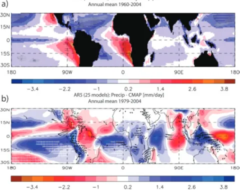
ost contemporary coupled atmosphere–ocean general circulation models (CGCMs) produce a climate that is significantly more symmetric about the equator than in observations (Mechoso et al.

1995; Davey et al. 2002; Biasutti et al. 2006; de Szoeke and Xie 2008; Richter et al. 2016; Richter 2015; Siongco et al. 2015). Outstanding features include positive sea surface temperature (SST) errors south-southeast of the equator (Fig. 1a), collocated in part with an inter- tropical convergence zone (ITCZ) precipitation band (Fig. 1b) much stronger than that observed in nature.

The “double ITCZ” error is further implicated in the simulated Hadley circulation, seasonal cycle and winds

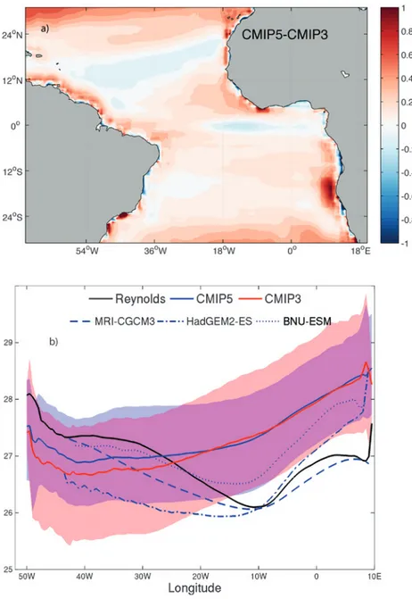
on the equator, and equatorial modes of variability, such as El Niño–Southern Oscillation (ENSO) in the Pacific, casting doubt on the ability to model and pre- dict both regional and global climate. These positive SST biases are apparent only in the Pacific and Atlantic basins (Fig. 1a), indicating the Indian Ocean’s precipitation biases have other origins. Phase 5 of the Coupled Model Intercomparison Project (CMIP5) models demonstrate only a slight improvement in the mean from CMIP3 [Fig. 2a; see also Richter et al. (2014b) and Zhang et al. (2015)], revealing the stubbornness of the biases, although some individual models are more successful (Fig. 2b; Richter et al. 2014b).

(2)

AFFILIATIONS: Zuidema, Kirtman, and Jung—University of Miami, Miami, Florida; Chang—Texas A&M, College Station, Texas, and Collaborative Innovation Center of Marine Science and Technology, Ocean University of China, Qingdao, China; medeiros and small—National Center for Atmospheric Research,* Boulder, Colorado; meChoso—University of California, Los Angeles, Los Angeles, California; sChneiderand wang—George Mason University, Fairfax, Virginia; toniaZZo—University of Bergen, Bergen, Norway; riChter—Japan Agency for Marine-Earth Sci- ence and Technology, Yokohama, Japan; bellomo—Columbia University, New York, New York; brandt—GEOMAR, Kiel, Germany; de sZoeKe—Oregon State University, Corvallis, Oregon;

Farrar—Woods Hole Oceanographic Institution, Woods Hole, Massachusetts; Kato—NASA Langley Research Center, Hampton, Virginia; liand Xu—Ocean University of China, Qingdao, China;

PatriCola—Texas A&M, College Station, Texas; wood—University of Washington, Seattle, Washington

* The National Center for Atmospheric Research is sponsored by the National Science Foundation

CORRESPONDING AUTHOR: Paquita Zuidema, Rosenstiel School of Marine and Atmospheric Science, University of Miami, 4600 Rickenbacker Causeway, Miami, FL 33149-1098

E-mail: pzuidema@rsmas.miami.edu

The abstract for this article can be found in this issue, following the table of contents.

DOI:10.1175/BAMS-D-15-00274.1 In final form 12 May 2016

Another interhemispheric asymmetry with which models have difficulty is subtropical stratocumulus clouds. The planetary stratocumulus decks are not symmetric about the equator, but rather about the ITCZ located at approximately 10°N. The equatorial climate is linked directly to the Southern Hemisphere’s subtropical highs and stratocumulus cloud decks through the westward trade winds (Ma et al. 1996;

Bellomo et al. 2014, 2015). The longwave stratocumulus radiative cooling further strengthens the tropical atmospheric circulation (Bergman and Hendon 2000;

Peters and Bretherton 2005; Fermepin and Bony 2014).

Global models have struggled to capture the low-level, geometrically thin but optically significant stratocumulus clouds. The lack of clouds may then seem to be an agent for the warm SST biases, by allowing excessive sunlight to reach the surface (e.g., Huang et al. 2007).

However, CMIP models often overcompensate by cooling excessively through their surface turbulent fluxes (de Szoeke et al. 2010; Xu et al. 2014b).

At the equator, the ocean’s thermocline structure is sensitive to atmospheric wind perturbations, and positive air–sea feedbacks amplify SST variability (Bjerknes 1966, 1969; Philander 1981; Zebiak and

Cane 1987). While Pacific zonal SST gradients tend to be realistic and have a magnitude comparable to the observation, those in the Atlantic can have the opposite sign to that observed (Fig. 2b). Gulf of Guinea SSTs can be too warm (Fig. 2b), with biases beginning in the boreal spring and peaking in summer (DeWitt 2005; Song et al. 2015). The smaller Atlantic basin means its equatorial climate is influenced by the monsoons over Africa, North America, and perhaps even Asia (Rodwell and Hoskins 1996; Okumura and Xie 2004; Siongco et al. 2015). More recently ap- preciated is that the most severe SST biases, reaching 6°–8°C, occur in the coastal southeast Atlantic (SEA) away from the equator (Xu et al. 2014a; Toniazzo and Woolnough 2014). Observational studies have suggested oceanic Kelvin waves link the equatorial and southeast Atlantic Oceans since Hirst and Hastenrath (1983), a process also diagnosed in CMIP5 models (Xu et al. 2014a).

A brief description of the two basins sets the stage for further discussing their physical processes. The Southern Hemisphere SST distributions differ, in keeping with a different spatial structure to the oceanic eastern boundary currents (Fig. 3) that reflects different bathymetry (Mazeika 1967) and land to- pography (Philander 1979). The surface winds stream toward the ITCZ in both basins (not shown), but the near-equatorial eastern basin coastal surface current is poleward in the Atlantic and equatorward in the Pacific (Fig. 3). The eastern Pacific boundary current ultimately merges with equatorial waters cooled by upwelling. In contrast, the equatorward Benguela Current off the coast of southern Africa is met by the warmer waters of the poleward Angola Current, form- ing the Angola–Benguela Front (ABF) that migrates seasonally between 15° and 17°S. Furthermore, a raised upwelling oceanic thermocline north of the ABF, the Angola Dome, has no counterpart in the southern Pacific (Doi et al. 2007).

The warm Atlantic near-equatorial waters co- incide with a reduction in the cloud fraction that does not exist in the Pacific (Fig. 4). To the south, the southern boundary of the stratocumulus decks abuts the northern edge of coastal atmospheric wind jets (Fig. 4). All basins possess significant low-level atmospheric coastal jets above oceanic upwelling regions, but these winds are most pronounced in the Southern Hemisphere. The wind spatial distribution is important for establishing the upwelling structure (Fennel and Lass 2007; Small et al. 2015).

In the southeast Pacific (SEP), the wind jet exit into the Arica Bight supports an elevated, cloudy coastal boundary layer (Zuidema et al. 2009). In the Atlantic,

(3)

the coastal surface winds south of 20°S are guided northwestward along with the Benguela Current by the convex Angolan–Namibian coastline (Nicholson 2010), and the stratocumulus deck is primarily offshore. The monthly mean SSTs are 1–2 K warmer in the southeast Atlantic than in the Pacific (Fig. 4b), reducing the monthly mean atmospheric lower-tropospheric stabilities accordingly.

Nevertheless, the SEA cloud fraction exceeds that of the SEP during the austral spring (Fig. 4c), despite being thinner clouds (Fig. 4d), coinciding with a time when the aerosol optical depth (AOD) over the SEA is also greater (Fig. 4f).

Our discussion cannot be fully comprehensive of this vast, complex, and long- studied problem (see also Richter 2015). The main goal is to articulate the ra- tionale for recommended near-future improvements in individual models’ mean

tropical climate. The following section (“The surface energy balance in models and observations”) further assesses the surface energy balance in models and observations. The “Main regional processes contributing to coupled climate model SST biases” section discusses regional error sources for the SST biases, selected for their perceived importance: the stratocumulus cloud deck, deep convection, oceanic eddies, surface winds, and model resolution. The “Model error growth attribution” section highlights attributing bias through evaluating fast versus slow SST error growth. The “Remote impacts of eastern tropical SST biases” section discusses the impact of basin-specific SST biases upon the global climate, and the “Gaps and recommendations” section concludes with recommendations.

THE SURFACE ENERGY BALANCE IN MODELS AND OBSERVATIONS. Differences in CMIP5 model-mean surface flux biases, shown in

Fig. 5 with respect to the objectively analyzed air–sea fluxes (OAFlux) product (Yu et al. 2008), suggest different processes dominate the SST biases in the two basins. The CMIP5 net radiative [shortwave (SW) and longwave (LW)] surface fluxes are more biased in the southeast Pacific, where they are spatially collocated with the thicker SEP cloud deck, than in the southeast Atlantic. In contrast, the turbulent (primarily latent heat) fluxes are more biased in the Atlantic, where they ultimately dominate the net CMlP5 surface flux biases. Analysis of Atmospheric Model Intercom- parison Project (AMIP) simulations has shown that even with observed SSTs, surface energy flux biases of the same sign remain, if reduced (Zheng et al. 2011;

Vanniere et al. 2014a; Xu et al. 2014a).

Issues with the surface flux products used to assess CGCM biases will also affect the assessment.

For example, OAFlux does not have a globally closed surface energy budget, in that the turbulent fluxes are derived from National Centers for Environmental F^ig. 1. (a) CMIP5 ensemble annual-mean SST error in the historical 1960–2004 integrations of 25 Fifth Assessment Report (AR5) coupled GCMs relative to the Hadley SST climatology. (b) CMIP5 ensemble 1979–2004 annual-mean precipitation errors in the same 25 models relative to Climate Prediction Center (CPC) Merged Analysis of Precipitation (CMAP) data, and mean wind (arrows) errors in 22 models relative to ERA-I 10-m winds. Arrows plotted only where all individual model wind errors fall within 90° from the mean. White hatching denotes areas where the sign of the error agrees in all models; black dots denote where all but one [Commonwealth Scientific and Industrial Research Organisation Mark 3.6.0 (CSIRO Mk3.6.0)] agree.

[Adapted from Toniazzo and Woolnough (2014).]

(4)

Prediction (NCEP) data and the radiation fluxes from the International Satellite Cloud Climatology Product (ISSCP). A further assessment uses data from two buoys that measure all the surface energy components of the net heat flux: the Woods Hole Oceanographic Institution Stratus buoy at 20°S, 85°W, and a Prediction and Research Moored Array

in the Tropical Atlantic (PIRATA; Bourlès et al.

2008) buoy at 10°S, 10°W (Fig. 4). Approximately 20 buoys worldwide measure the full surface energy budget, with the primary limi- tation being the availability of a pyrgeometer (longwave radiation sensor), as it is difficult to calibrate and maintain (Yu et al. 2013).

Our assessment neglects spatial weighting issues (Josey et al. 2014).

Figure 6 shows the buoys’

climatological annual cycle, the OAFlux, and the Clouds and the Earth’s Radiant Energy System (CERES) surface radiative fluxes (Kato et al. 2013). The buoy radiation measurements indicate more surface longwave radiation loss, and less shortwave radiation flux going into the ocean, than in either the CERES or OAFlux dataset, consistent with Fig. 8 of de Szoeke et al. (2010). The shortwave bias is generally larger than the longwave bias, leading to an approximate positive bias (an ocean warming) in the net heat flux of 10 W m⁻² at the cloudier Stratus site.

A more quantitative comparison of the buoy, CERES, and OAFlux annual means is shown in Table 1, and includes values from the European Centre for Medium-Range Weather Forecasts (ECMWF) interim reanalysis [ERA-Interim (ERA-I)] and the TropFlux project. TropFlux is a gridded energy-balanced surface flux product developed explicitly to drive ocean dynamical simulations.

TropFlux combines ERA-I with ISCCP shortwave fluxes and includes buoy-based bias and amplitude corrections (Kumar et al. 2012, 2013). Buoy, OAFlux, and TropFlux turbulent flux calculations all rely F^ig. 2. (a) CMIP5 minus CMIP3 model-mean SST differences reveal little

improvement, while (b) the equatorial Atlantic SST gradient is only slightly improved in CMIP5 (blue) from CMIP3 (red; solid line denotes model mean and color-fill denotes standard deviation), with the Reynolds climatological mean values as the black line. The three models capable of reproducing the correct asymmetry are highlighted [Meteorological Research Institute Coupled Atmo- sphere–Ocean General Circulation Model, version 3 (MRI-CGCM3), Hadley Centre Global Environment Model, version 2–Earth System (HadGEM2-ES), and Beijing Normal University–Earth System Model (BNU-ESM)].

(5)

on the Coupled Ocean–

Atmosphere Response Experiment (COARE), version 3, bulk algorithm (Edson et al. 1998; Colbo and Weller 2009). CERES, OAFlux, and ERA-I report a larger net radiation flux into the ocean than the buoy at both locations, with the CERES–buoy difference exceeding the reported CERES uncertainties (Kato et al. 2013). In contrast, TropFlux does not allow enough radiation to enter the ocean.

T he ove re s t i m at e d OAFlux net radiative fluxes combine with underes- timated turbulent fluxes to yield too much net surface warming, by almost 20 W m⁻², at both buoy sites.

In contrast, weak TropFlux and ERA-I net fluxes do not warm the ocean enough at

the Stratus buoy location, by 10–25 W m⁻², primarily because the turbulent fluxes overcompensate. At the Atlantic PIRATA buoy, the ERA-I net fluxes similarly do not produce enough warming, but here the individual biases in the TropFlux fluxes compensate to yield a reasonable net flux. Overall the ERA-I—and,

to a lesser extent, TropFlux—biases are similar in sign to that of CMIP3 models (not enough ocean warming; de Szoeke et al. 2010). An annual-mean 2001–09 time series of the Stratus buoy and OAFlux surface flux components confirms the consistency of the OAFlux (ISCCP) radiation biases (Fig. 7). An Fig. 3. The surface currents help bring colder waters up near the equator in the Pacific, whereas in the Atlantic, the warm Angola Current flows south from the equator to 15°S, establishing a strong SST gradient with the northward-flowing cool Benguela Current to its south. Annual-mean SST and surface current data from the Simple Ocean Data Assimilation reanalysis.

Table 1. Annual-mean surface fluxes (W m⁻²) from buoy, CERES, OAFlux, TropFlux, and ERA-I da- tasets. Net CERES fluxes in parentheses are calculated using the OAFlux turbulent fluxes. All values are positive downward. The buoy turbulent fluxes are calculated using the COARE 3.0 bulk formulas, with an estimated error of 5 W m⁻² (Colbo and Weller 2009; Edson et al. 1998). These algorithms are also used in OAFlux and TropFlux. The Stratus buoy sensors were evaluated and calibrated annually for 9 yr (Colbo and Weller 2007; Holte et al. 2014).

Stratus (20°S, 85°W)¹ PIRATA (10°S, 10°W)²

Net SW Net LW Net SW + LW SH + LH SH Net Net SW Net LW Net SW + LW SH + LH SH Net

Buoy 191.0 −42.6 148.4 −111.9 −7.4 36.5 219.8 −48.7 171.1 −150.5 −5.4 20.6

CERES 201.1 −39.4 161.7 — — (52.4) 224.7 −49.5 175.2 — — (38.0)

OAFlux 195.3 −30.0 165.3 −109.3 — 56 223.0 −42.3 180.7 −137.2 −9.9 43.5

TropFlux 175.8 −42.7 133.1 −121.2 −16.8 11.9 209.5 −46.4 163.1 −143.3 −12.0 19.9

ERA-I 207.0 −47.0 160.0 −137.8 −15.4 21.8 229.1 −51.0 178.1 −170.7 −15.0 7.7

1 1 Jan 2001–31 Dec 2009.

2 1 Jan 2009–31 Dec 2009.

(6)

interesting increase in the turbulent fluxes is attrib- uted to increasing winds by Weller (2015), which are more weakly apparent in the OAFlux time series.

Net gridded flux terms indicate either too little or too much heat going into the ocean, by ±10–20 W m⁻², com- pared to buoy values, depending on the product. This influences the interpretation of CMIP model surface energy budget biases. The main constraint on using buoy data for climate model validation is the lack of longwave radiation data and data gaps.

MAIN REGIONAL PROCESSES CONTRIB- UTING TO COUPLED CLIMATE MODEL SST BIASES. OAFlux allows for more ocean warm- ing than is observed, an error that implies the CMIP5

model net flux biases are even larger, by at least 10 W m⁻², than reported in Fig. 5. This only reinforces the sense of the net CMIP5 errors, particularly in the cloudier regions. We next focus on how the CGCM representations of clouds, deep convection, oceanic eddy mixing, winds, and the model resolution contribute to perceived model SST biases.

Clouds. Improvements in cloud radiation fields improve the equatorial climate through altering equatorial winds, SSTs, and ITCZ rainfall (Ma et al. 1996;

Hu et al. 2008; Wahl et al. 2011). More recently the underrepresentation of clouds in the Southern Ocean has also been linked to the spurious double ITCZ in CMIP models (Hwang and Frierson 2013). The cloud measure most directly relevant to the surface Fig. 4. The September-mean SST, cloud, and coastal wind climatology, and annual cycle in cloud and atmospheric properties for the two basins. (a) Based on 2000–10 September-mean SST (°C) from the TRMM Microwave Im- ager (colored contours), 2001–10 Moderate Resolution Imaging Spectroradiometer (MODIS; Terra) cloud fraction (gray-filled contours, values spanning 0.6–1.0), and 1999–2009 QuikSCAT coastal wind maxima (yellow-red-filled contours, values spanning 7.5–9.0 m s⁻¹, isolated from other wind speed maxima). Domain-mean annual cycles in (b) SST, (c) cloud fraction, (d) daily mean liquid water paths, (e) LTS (here, the 2000–10 ERA-I 700–1000-hPa po- tential temperature difference), and (f) MODIS aerosol optical depths shown for the two indicated boxes: 10°–20°S, 80°–90°W and 10°–20°S, 0°–10°E averages, following Klein and Hartmann (1993). Liquid water paths from 2002–11 Advanced Microwave Scanning Radiometer for Earth Observing System (AMSR-E). Locations with indicated buoys (Stratus and 10°S, 10°W) are assessed in “The surface energy balance in models and observations” section.

(7)

energy balance is the cloud impact on the radiation.

A cloud radiative effect (CRE), defined as the difference between the net top-of-atmosphere radiation (longwave plus shortwave) when clouds are present and when clouds are absent, can be directly compared to satellite-derived values. The CRE avoids compli- cations in different cloud cover measures (Kay et al.

2012), although models tuned to produce a “reasonable” CRE pattern may compensate between cloud cover and optical thickness (Nam et al. 2012). Mean CMIP5 net CRE biases are very large, up to 40 W m⁻², relative to CERES values (Figs. 8a and 8b; see also Lin et al. 2014). This is especially the case in the Pacific, consistent with Fig. 5. The CMIP5 models generally continue to underestimate subtropical stratocumulus cloud cover relative to observations (Fig. 9), similar to CMIP3 (Klein et al. 2013), although fewer subtropical clouds are overly optically thick (Klein et al. 2013).

A natural question to ask is whether the strong SST bias initially creates the cloud bias, or vice versa.

The CMIP5 archive also includes atmosphere-only simulations that prescribe observed SST (the so-called AMIP simulations). These provide a test of the model’s atmospheric errors, with cloud errors coupled with the circulation but not with the SSTs. The AMIP ensemble-mean CRE bias relative to CERES shows remarkable similarity to the coupled GCM results.

Closer inspection reveals that the biases in the coupled models do tend to be larger than in the AMIP models, suggesting some role for surface temperature feedbacks in exacerbating the atmosphere’s cloud bias

(Figs. 8e and 8f). In addition, more of the AMIP simulations show negative biases, which implies that fixing the SST can lead to an overcorrection in the clouds, a feature also noted in some regional climate models (Richter 2015). The atmospheric model component is thus implicated as the main cause of the cloud errors (see also Lauer and Hamilton 2013).

The question is then whether climate models fail to produce the large-scale conditions conducive to cloud formation, in particular the lower-tropospheric stabil- ity (LTS), or if climate models struggle to depict low clouds realistically even when the large-scale circulation is correct. Most CMIP5 models possess a lower troposphere over the stratocumulus regions that are less stable than in ERA-I, but with reasonable seasonal phasing (Figs. 9e and 9f). Yet, many CMIP5 model annual cycles in stratocumulus cloud amount and liquid water path are opposite of that in observations (Figs. 9a–d), with too much cloud during January–

March, when the atmosphere is less stable. Models with stronger correlations between low cloud cover and the LTS generally possess more realistic cloud annual cycles (see also Noda and Satoh 2014; Lin et al. 2014).

In Fig. 9, the Community Earth System Model, version 1 {Community Atmosphere Model, version 5 [CESM1 (CAM5)]} is best able to reproduce a realistic seasonal cycle. In CAM5, underestimates of the offshore stratocumulus can be thought of as an overeager transition to trade cumulus (Medeiros et al.

2012). Near the coast, land-induced subsidence significantly adds to the larger-scale subsidence (Muñoz F^ig. 5. (a)–(d) CMIP5 biases for the eastern Pacific show different spatial structures than those for the eastern Atlantic. (a),(e) Net SW, (b),(f) net LW, (c),(g) turbulent [sensible plus latent heat (SH + LH) fluxes], and (d),(h) net surface flux CMIP5 biases averaged from 1984 to 2004 relative to OAFlux. (i),(j) CMIP5 SST biases relative to the Reynolds climatology. Buoy locations considered in Figs. 6 and 7 and Table 1 are indicated with black and yellow boxes, respectively.

(8)

A

long history of interest exists in solving “the double-ITCZ problem,”

beginning with meetings in the late 1980s–early 1990s focused on the Pa- cific, co-organized by George Philander and others in Toledo, Spain, then Paris, France, and later in Los Angeles, Cali- fornia (Mechoso et al. 1995; Mechoso and Wood 2010). A consensus that available datasets for the eastern tropical Pacific were not sufficient to support a detailed model validation spawned the 1995–2005 U.S. PanAmerican Climate Studies (PACS) program, which oversaw the development of the Eastern Pacific Investigation of Climate Processes in the Coupled Ocean–Atmosphere System (EPIC) field campaign in 2001.

EPIC connected observations in the eastern Pacific ITCZ (Raymond et al.

2004) to the stratocumulus-covered southeastern Pacific (Bretherton et al.

2004b). The newly created panel on VAMOS of the World Climate Research Programme (WCRP)’s U.S. Climate Variability and Predictability Program (CLIVAR) thereafter developed and implemented the more comprehensive VOCALS Regional Experiment held in 2008 (Mechoso et al. 2014). This com- prehensively documented the southeast

Pacific aerosol–cloud environment, and VOCALS datasets have been used to constrain climate model microphysics (Gettelman et al. 2013) and turbulence (Kubar et al. 2015). A subsequent workshop in 2011 focused on the physical processes underlying model biases in the tropical Atlantic (Zuidema et al.

2011a,b).

In parallel with PACS, meetings more specifically focused on the performance of CGCMs continued. A 2003 meeting directed by the National Science Foundation (NSF) specifically sought a modeling strategy for reducing the biases through a “mini-CMIP” multimodel comparison, followed by workshops in 2005–07. A further concept intro- duced at the 2003 meeting was to bring smaller teams of observationalists and modelers together in climate process teams (CPTs), to develop and improve relevant and specific model parameterizations (Bretherton et al. 2004a). CPTs, with lifetimes of approximately 3 years, have addressed cloud parameterizations, oceanic deep mixing, and oceanic eddies to date, building on datasets from the southeast Pacific and the oceanic Dia- pycnal and Isopycnal Mixing Experiment in the Southern Ocean (DIMES).

U.S. oceanographic activity in the Atlantic primarily occurs through cooperation with France and Brazil in PIRATA (Bourlès et al. 2008), as well as within internationally coordinated multiyear process studies focusing on the eastern equatorial Atlantic cold tongue [see Johns et al. (2014), and corresponding special issue] and the variability of the African monsoon [African Monsoon Multidisciplinary Analysis (AMMA); see also Roehrig et al. 2013]. A recent large European Union consortium is now conducting the oceanographic Enhancing Pre- diction of Tropical Atlantic Climate and Its Impact (PREFACE) campaign, focusing on the near-coastal southeastern Atlantic SST bias. Significant atmospheric fieldwork in the southern Atlantic, originating largely outside of the WCRP CLIVAR framework, is now underway (Zuidema et al. 2016). These campaigns are part of a strategy to understand low-cloud adjustments to biomass-burning aerosols from African continental fires and further feedbacks to regional climate. Efforts to improve SST biases in global aerosol models will improve climate simulations of the aerosol effects as well.

A 30-YEAR HISTORY CONTINUES

and Garreaud 2005; Toniazzo et al. 2011), generating a positive correlation between boundary layer depth and cloud cover that contrasts with that offshore (Garreaud and Muñoz 2005). Model intercomparisons in the southeast Pacific reveal model underestimates in the near-coastal boundary layer depth (Wyant et al.

2010, 2015), related to relatively low model vertical resolution and poor treatment of cloud-top entrainment mixing in some models (Sun et al. 2010). The dynamic and thermodynamic environments occupied by the coastal and offshore stratocumulus regions may be best considered individually, particularly for the Pacific (Fig. 4). The direct radiative effect of aerosols as a cause for SST biases must be small simply because aerosol optical depths are small compared to that of clouds (Fig. 5f). Interest in aerosol–cloud interactions nevertheless aid useful low-cloud parameterizations efforts (e.g., Mechoso et al. 2014; see also the sidebar).

The atmospheric model component is implicated as the cause for too few low clouds in coupled models.

Deep convection. Tropical precipitation in coupled climate models is offset from observations (Fig. 1b), and the large-scale circulation links the precipitation to the SST biases. In and around the smaller Atlantic basin, South America and Africa also compete for the precipitation, affecting the hemispheric distribution, evident in AMIP runs already (Siongco et al. 2015).

Although the process(es) linking the precipitation and SST biases is (are) still under debate (Richter and Xie 2008; Zermeno-Diaz and Zhang 2013; Richter et al. 2014a), it is self-evident that models with better precipitation representations can more accurately capture realistic air–sea coupling.

The question arises whether the convective parameterizations are themselves to blame for the precipitation biases, or whether other model aspects affect how the precipitation is distributed. Little progress is evident moving from CMIP3 to CMIP5 (Zhang et al. 2015), despite significant efforts to improve some of the convective parameterizations (e.g., Gent et al. 2011). Increases in model resolution (both atmospheric and oceanic)

(9)

do slightly improve the precipitation placement (Gent et al. 2011; Patricola et al. 2012), related by Siongco et al. (2015) to an improved continental geography sur- rounding the Atlantic basin but not to the convective parameterizations. It is only at resolutions that begin Fig. 6. The mean annual cycles in the net SW, net LW, turbulent (SH + LH) fluxes, and their sum (net) at the (a) Stratus WHOI buoy (20°S, 85°W) and (b) PIRATA (10°S, 10°W) buoys (see also Figs. 4 and 5), from buoy data (black solid line), CERES Energy Balanced and Filled (EBAF) radiation data (red and blue solid lines), and OAFlux (ISCCP) data (dashed and green solid lines).

Annual-mean buoy values are indicated to the right of each panel. The Stratus buoy annual cycles are based on complete data spanning 1 Jan 2001–31 Dec 2009, while the PIRATA buoy annual cycles span intermittent and differing time lengths: Mar 2000–Nov 2013 for CERES, Oct 1997–May 2014 for the buoy turbulence and SW radiation data with occasional data gaps, and Aug 2005–

May 2014 for the buoy LW radiation data with missing data in 2011–12. The OAFlux dataset spans 1985–2009.

The CERES EBAF data have a resolution of 25 km, and the OAFlux dataset has a 1° resolution, averaged over 2° × 2° at the two buoys.

to permit convection explicitly—10 km or less—that convective representations clearly improve (Dirmeyer et al. 2012), supporting the use of a multiscale modeling framework that intersperses explicit simulations of convection into climate models (Randall et al. 2003).

Until climate model resolutions of 10 km or less are readily available to many, efforts to improve convective parameterizations remain warranted. A well- known shortcoming of cumulus parameterizations is their insensitivity to the environmental air and particularly to humidity (Derbyshire et al. 2004; Del Genio 2012). This curtails climate models’ ability to capture the full range of ITCZ convective variability (shallow, congestus, and upper-level stratiform in addition to the prototypical deep convective towers) and mesoscale organization. The inability to represent small-scale convection–humidity interactions (entrainment, rain evaporation) affects the sensitivity of ITCZ precipitation to larger-scale local changes versus remotely driven changes in the atmospheric thermodynamics. Higher grid resolutions challenge a basic assumption of most convection schemes—

namely, that the updraft fraction is small within a grid box, introducing new difficulties in parameterizing mesoscale organization (Arakawa 2004; Arakawa et al. 2011; Del Genio 2012). Convection–humidity interactions may be particularly difficult to capture well for the narrow Atlantic and eastern Pacific ITCZ regions because of their strong meridional SST and free-tropospheric pressure and humidity gradients (Zuidema et al. 2006; Zhang et al. 2008).

Some skill in reproducing observed relationships between convection, relative humidity, and vertical ve- locity has been demonstrated using stochastic physics (Watson et al. 2015). Systematic biases in model physics can also be uncovered through comparison to observations at high temporal and vertical resolution (Phillips et al. 2004; Webb et al. 2015; Nuijens et al. 2015).

Efforts to improve tropical precipitation biases require both increased model resolution and sustained param- eterization development in individual models.

Oceanic eddy mixing. Warm SST biases are also apparent—if sharply reduced—in ocean model–only [Ocean Model Intercomparison Project (OMIP)] simulations forced using realistic atmospheric forcing estimates, such as the Common Ocean Reference Experiment, version 2 (CORE2; Yeager and Large 2008); see Fig. 10.

This suggests that model ocean processes also do not provide sufficient surface cooling. Furthermore, an early assessment of 4 years’ worth of subsurface data from the Stratus buoy suggested the mean ocean

(10)

Fig. 7. The 2001–09 annual-mean time series in (a) net SW, (b) net LW, (c) turbulent (SH + LH) fluxes, and (d) their sum (net) at the Stratus WHOI buoy (20°S, 85°W) spanning 2001–09, using buoy data (black solid line), CERES EBAF radiation data (colored solid lines), and OAFlux (ISCCP) data (dashed lines). Mean values are shown at right.

circulation did not advect enough cool water to balance the time-mean upper-ocean heat budget (Colbo and Weller 2007, 2009). These observations motivated work during the Variability of the American Monsoon Systems (VAMOS) Ocean–Cloud–Atmosphere–Land Study (VOCALS) to understand the role of ocean eddies in redistributing heat.

Subsequently, several regional eddy-resolving ocean modeling studies have highlighted the contribution of eddies to the SST (Colas et al. 2012, 2013), most pronounced within several hundred kilometers of the South American coast, but with little influence by eddy transport over 1,000 km offshore (Toniazzo et al.

2009; Zheng et al. 2010, 2011). A longer buoy time series providing an additional 5 years of data, combined with Argo floats, drifters, and satellite altimeter data, now suggests that the mean oceanic circulation, rather than eddies, does provide sufficient surface cooling 1,000 km offshore (Holte et al. 2013, 2014).

An important lesson may be that one isolated buoy is not adequate for robustly determining an eddy contribution. A long time series, approaching 20 years, is needed to establish the mean upper- oceanic heat budget because of the slow evolution of individual eddies. This is because the three or four eddies passing a buoy annually provide consid- erable interannual and perhaps even interdecadal variability to the terms in the upper-ocean heat budget. More crucially perhaps, other means are required to establish the spatial context. Modeling challenges still remain, as robustly modeling oceanic eddies requires high resolution at both the spatial and vertical scales and attention to diffusion and numerical schemes. The emergent properties of ed- dying versus noneddying models may allow for a more definitive evaluation of the effect of eddies.

Atlantic turbulent fluxes are more biased than in the Pacific, with large near-coastal model SST biases (Fig. 5j) that are not collocated with the shortwave errors (Fig. 5e). This is consistent with ocean models contributing more to the SST biases in the Atlantic than the Pacific, in keeping with Xu et al. (2014a). For the coastal region, the extent of the eddy contribution to maintaining the Angola–Benguela Front is still unknown but may be significant, given the strong frontal structure and density gradient (Fig. 3).

Available evidence now suggests a contribution by oceanic eddy mixing to SEP SST 1,000 km offshore that is less than the still significant sampling error from one buoy, while the contribution of eddies to the SEA SST is still unknown.

Winds and model resolution. The history in understanding the wind contribution to SST error growth

(11)

▶ F^ig. 8. (top) Composite annual-mean net CRE biases with respect to CERES values reveal larger cloud ra- diative biases in (a) the Pacific than in (b) the Atlantic, based on 22 CMIP5 models. The largest biases occur at the coast. (middle) Fixed-SST (AMIP) simulations re- veal similar annual-mean cloud biases in (c) the Pacific and (d) the Atlantic, implicating the atmosphere as the source for low-cloud errors, based on 28 models span- ning 1950–99 when available, with most simulations beginning in 1979. The AMIP ensemble is composed of different models than the CMIP5 ensemble, based on data availability. (bottom) CREs from atmosphere- only vs coupled simulations of the same model are compared in (e) the Pacific (10°–20°S, 80°–90°W) and (f) the Atlantic (10°–20°S, 0°–10°W), where the dashed line indicates y = x. CMIP5 “historical” simulations span 1950–99, all months, and CERES EBAF [Edition 2.8 (Ed2.8)] spans 2000–13. No attempt is made to account for model independence (Caldwell et al. 2014).

is closely tied to that of model resolution. Along the equatorial Atlantic, the most robust process contribution to SST error growth occurs through reinforc- ing too-weak easterlies. The wind bias is linked to incorrect model-dependent distributions of tropical precipitation (Biasutti et al. 2006; Richter and Xie 2008; Richter et al. 2012; Siongco et al. 2015) and is also present in AMIP simulations (e.g., Zermeno-Diaz and Zhang 2013), although the ocean model can also contribute through too-weak entrainment through the ocean thermocline (Song et al. 2015).

The most significant improvements in the equatorial climate have come from improvements in model resolution both in the atmosphere and ocean, argu- ably first noted in the eddy-resolving regional ocean simulation of Seo et al. (2006). Equatorial and eastern Pacific SSTs improved in higher-resolution versions of the Community Climate System Model (CCSM;

McClean et al. 2011) and the Geophysical Fluid Dynamics Laboratory Climate Model, version 2.5 (GFDL CM2.5; Delworth et al. 2012). A notable suc- cess is the first realistic climate model depiction of the Atlantic cold tongue and ITCZ location using a high- resolution version of CESM (Small et al. 2014). Thus, equatorial SST biases ultimately appear solvable once individual CGCMs can acquire sufficient resolution in their individual atmosphere and ocean components to resolve the dynamics unique to the equator. That said, a remaining question is how the equatorial Atlantic westward winds are maintained when they oppose the sea level pressure gradient (Richter et al. 2016).

Improvements in the equatorial winds do, through coastal Kelvin waves, improve the coastal climate at the eastern basin boundaries (Richter et al. 2012). However, this is not sufficient to remove the coastal SST biases

altogether, in particular in the southeast Atlantic.

Further work has clarified that increased resolution in the atmospheric model component is more important than in the oceanic component, once the latter is on the order of 0.25° resolution (Fennel and Lass 2007;

Small et al. 2014, 2015).

The relationship between model resolution and SST biases is explored in Fig. 11 using low- and high-resolution versions of the CCSM4 and CESM1 (CAM5). The low-resolution models are approximately 1° in both the atmosphere and ocean, while the two higher-resolution versions both possess 0.1°-resolution oceans, but a 0.5°

(12)

F^ig. 9. CMIP5 model seasonal cycles (gray lines) in stratocumulus cloud are often out of phase with observations.

Total/low-cloud amount in southeast (a) Atlantic and (b) Pacific, liquid water path in southeast (c) Atlantic and (d) Pacific, and LTS (θ700hPa minus θ1000hPa) in southeast (e) Atlantic and (f) Pacific. In (a) and (b), MODIS low cloud indicated in blue, ISCCP total cloud in red, and International Comprehensive Ocean–Atmosphere Data Set (ICOADS) surface observations of total cloud cover in aqua [Hadley Centre Global Environmental Model, version 2—Atmosphere (HadGEM2-A)] In (c) and (d), AMSR-E 2002–12 liquid water paths are in red. Models most highly correlated with observations are highlighted in black and labeled [Beijing Climate Center, Climate System Model, version 1.1 (moderate resolution) and Australian Community Climate and Earth-System Simu- lator, version 1.0 (ACCESS1.0)]. The model with the highest dual correlation is CESM (CAM5) and CSIRO is second. Domains are as shown in Fig. 4.

atmosphere for CCSM4 (Kirtman et al. 2012) and 0.25°

atmosphere for CESM1 (CAM5) (Small et al. 2014).

Both high-resolution simulations show improvements in the broader, more meandering western boundary currents, with the overall warm bias in the CCSM4 simulation reflecting a large sea ice melt event. The narrower, more coastal-hugging southeast Atlantic coastal region is basically unchanged with improvement in ocean resolution in the CCSM4 simulations.

The CESM (CAM5) high-resolution model, with a 25-km atmosphere, does show clear improvement over the low-resolution version, also in the southeast Atlantic region. Nevertheless, the improvement may not be happening for the right reasons. The way the Parallel Ocean Program, version 2 (POP2), receives the wind data includes partially land-covered atmosphere cells that bias the wind speed low close to the coast, and an area of large wind stress curl is created between the coast and the offshore atmospheric jet, displacing the location of the upwelling offshore.

The sensitivity of the upwelling to the structure of the coastal winds is shown for a regional climate model in Xu et al. (2014b) and by embedding a high-resolution ocean model within the CCSM4 in Small et al. (2015).

Part of the warm coastal SST bias is related to meridional ocean transport by an erroneous warm southward current near the coast that is forced by an excessive cyclonic wind stress curl. Indeed, Xu et al. (2014a) attribute approximately 50% of the southeast Atlantic SST bias to the poor simulation of the wind stress curl in CMIP5 models. The excessive cyclonic wind stress curl then forces an erroneous warm southward coastal current (Xu et al. 2014a; Small et al. 2015). The largest model SST improvements were found by adjusting the model coastal wind structure to observations within a narrow (2°) coastal zone (Small et al. 2015).

The differences in how CMIP5 models, the ocean- forcing CORE2 dataset, and satellite winds resolve the surface winds and their stress curl for the coastal southeast Atlantic are shown in Fig. 12. The CMIP5

(13)

winds and stress curl region is broad and pronounced, with the wind stress curl maximum displaced too far offshore, related by Richter (2015) to the offshore placement of the CMIP5 winds and too-weak near-coastal CMIP5 winds. The importance of the spatial wind distribution (Jin et al. 2009) can mean that even the reanalysis-derived CORE2 surface forcing dataset, with its approximately 1°–1.5° spatial resolution (Fig. 12b; Large and Yeager 2008), will ad- versely affect OMIP simulations when compared to the Scatterometer Climatology of Ocean Winds (SCOW;

Fig. 12a; Risien and Chelton 2008). Only at a spatial reso-

lution of approximately 10 km do the two wind maxima evident in the SCOW climatology become fully resolved (Fig. 12d).

The problem of adequately attributing causes is particularly complex near the Benguela upwelling region, because the Angola–Benguela Front is also not well resolved in CMIP5 models. A southward displacement of the Angola–Benguela Front occurs in all CMIP5 models and is correlated to the strength of the SST biases (Xu et al. 2014a). Too-diffuse coastal and equatorial thermoclines and warm subsurface temperature biases at the equator reinforce the southeast SST bias (Xu et al. 2014b; Small et al. 2014; Richter 2015).

Equatorial SST biases become mitigated with higher model resolutions, whereas eastern basin coastal SST biases are alleviated more by resolution improvements in the atmosphere surface wind stress, once the ocean model component is adequately resolved.

MODEL ERROR GROWTH ATTRIBUTION.

Interim solutions for SST bias identification and cor- rection include prescribing observed quantities for some variables, such as clouds (Huang et al. 2007;

Hu et al. 2008) or surface radiative fluxes (Wahl et al.

2011). Other studies assess process biases through correlations and lead–lag analyses (Richter and Xie 2008). More recent efforts evaluate the evolution in time of the systematic departure from well-defined initial conditions (observations or reanalysis) to

identify the processes responsible for the initial fast SST error growth. These are termed “initial tendency”

assessments when data assimilation is applied to identify the forecast error (Klinker and Sardeshmukh 1992; Rodwell and Palmer 2007), and hindcast or

“transpose AMIP” (Williams et al. 2013) when weather forecasts assess fixed-SST models initialized with conditions common to a weather forecasting center.

In coupled models, similar decadal hindcast experiments can assess both fast and slow SST error growth over time scales between days and a few years (Toniazzo and Woolnough 2014). Errors more directly linked to the model can then be identified before larger- scale coupled feedbacks and remote influences over- whelm the error structure in long-term simulations.

This is particularly effective for assessing the impact of parameterized fast processes, such as clouds and turbulence, on the SST error growth (Ma et al. 2014). The initialization must reflect the full ocean–atmosphere system, and the biases calculated with respect to the same dataset used for the initialization. Care must also be taken that the error growth is not simply “initialization shock” (Klocke and Rodwell 2014). A challenge remains to establish realistic initial conditions (Ma et al. 2015); an alternative, albeit a technically more demanding approach, is to analyze variable increments in data assimilation systems (e.g., Jung 2011).

An ensemble-mean example from CCSM4 highlights that errors after 5 days can show the initial seeds of a warm bias that develops a year later in the Fig. 10. Ocean simulations with fixed atmosphere forcings (termed OMIP) also produce SST biases, if less pronounced than in CMIP simulations, as shown in the 22-ensemble OMIP SST bias relative to CORE2 surface forcing for (a) the Pacific and (b) the Atlantic (Danabasoglu et al. 2014). This suggests oceanic origins also contribute to the SST biases.

(14)

Fig. 11. SST biases from low-resolution (approximately 1° in both the ocean and atmosphere) (a) CCSM4 and (b) CESM1 (CAM5) simulations and from high-resolution (c) CCSM4 (Kirtman et al. 2012) and (d) CESM1 (CAM5) (Small et al. 2014) simulations. The high-resolution CCSM4 coupled simulation uses a 0.1° ocean with 42 oceanic levels and a 0.5° atmosphere, and the high-resolution CESM1 (CAM5) model uses a 0.1° ocean with 62 levels, a 0.25° atmosphere, and a spectral element dynamical core. Both high-resolution simulations use POP2 (Danabasoglu et al. 2012). The low-resolution simulations are averaged from 1850 through 2005 and are compared with the 1850–2005 merged Hadley–Optimum Interpolation Sea Surface Temperature (OISST) climatology (Hurrell et al. 2008). The high-resolution simulations are compared with 10-yr-mean observed SSTs centered on the appropriate observed annual-mean CO₂ concentration [1986–1995 for CCSM4’s imposed CO₂ forcing of 355 parts per million (ppm) and 1996–2005 for CESM1 (CAM5)’s CO₂ 367-ppm forcing].

southeastern Pacific, despite differences in the overall error structure (Fig. 13). The initialization is done with NCEP’s coupled reanalysis product, the Climate Forecast System Reanalysis (CFSR; Saha et al. 2010), which is generated from a coupled seasonal climate forecasting system, the Climate Forecasting System, version 2 (CFSv2; 2011; Saha et al. 2014), and its ad- joint; a weakness remains the deficit in the low-cloud CRE (Hu et al. 2008). In a more thorough analysis of three models within the CMIP5 database (Toniazzo and Woolnough 2014), large surface wind biases were the first to appear, especially over the equatorial region, driving many of the subsequent errors. These initial wind errors are generally coupled with areas of deep convection (Richter et al. 2012), suggesting that atmospheric circulation errors coupled with model

physics, especially tropical convection, originate the short-term systematic biases.

Analysis of fast SST error growth processes is a promis- ing computationally efficient approach for pinpointing the importance of parameterized fast processes, such as convection, clouds, and turbulence, to short-term SST error growth.

REMOTE IMPACTS OF EASTERN TROPI- CAL SST BIASES. What is the impact of the individual basin SST biases upon the SST and precipitation distribution outside of the basin? This is important to gauge in individual models, toward establishing model development priorities. Large and Danabasoglu (2006) concluded that within-basin

(15)

impacts of the coastal biases, through surface current advection of the coastal SSTs, are substantial. At an intermediate stage of complexity between fully coupled and AMIP/OMIP experiments, we performed similar experiments with a succession of atmospheric models {Community Atmosphere Model, version 3.0 [CAM3.0 (T42; Xu et al. 2014a)], CAM4 (2° × 2°), and CAM5 (2° × 2°)} coupled to a slab ocean, meaning ocean dynamical adjustments are neglected. First, a surface heat flux representing the divergence of the ocean heat flux together with biases in the atmospheric model processes (commonly called the Q flux) is found, which, when included in the forcing of the ocean, produces a modeled annual-mean SST climatology matching the observed SST. Then, two further SST bias simulations set the Q flux to zero—in an Atlantic region in one case and in a Pacific region

in another case—while applying the original Q flux (adjusted by a constant to preserve the global-mean Q flux) everywhere else. As is evident in Fig. 14, the Q flux differences (negative changes correspond- ing to heating and positive changes to cooling) are smaller in magnitude in the CAM5 experiment than in CAM4, and in CAM4 than in CAM3, for both the Atlantic and Pacific cases, indicating a reduced role for the ocean heat fluxes and atmospheric process biases going from CAM3 to CAM4 to CAM5.

In both experiments, large SST biases appear in those regions where the Q flux is set to zero.

Everywhere else, the changes in surface temperature and precipitation result from the remote influence of the original bias. The local impact of the Atlantic Q flux adjustment on the SST is prominent, in agreement with Small et al. (2015). The precipitation impact in Fig. 12. Coastal southeast Atlantic (a)–(d) meridional winds at 10 m and (e)–(h) surface wind stress curls differ significantly between observations and models and depend on spatial resolution: (a),(e) 0.25° SCOW ocean surface wind vectors, averaged 1999–2009; (b),(f) 1° CORE2 ocean forcing dataset, averaged 1999–2009; (c),(g) CMIP5 multi- model mean, averaged 1984–2004; and (d),(h) a 9-km simulation with the Weather Research and Forecasting Model, averaged 2005–08. See further discussion in Patricola and Chang (2016, manuscript submitted to Climate Dyn.).

(16)

Fig. 13. (a) Fast and (b) slow SST error growth, de- rived from a 10-member ensemble of retrospective CCSM4 forecasts initialized every 12 h starting at 0000 UTC 27 Dec of each year from 1982 to 2009 with NCEP’s coupled reanalysis product CFSR (Saha et al.

2010), showing similarities between the (a) mean SST anomaly error of all the forecasts averaged over the first 5 days and (b) error average from days 361 to 365.

Both represent an average over 1370 forecast days.

CAM3 exhibits a pronounced southward shift of the Atlantic ITCZ as well as a northward shift in the Pacific low-latitude precipitation. The impact on precipitation in CAM4 has a structure similar to that in CAM3 but with weaker amplitude, while the impact on precipitation in CAM5 is an east–west dipole rather than a north–south shift in the Atlantic, with little remote impact in the Pacific. In the Pacific Q flux experiments, all three model versions show eastern Pacific warm bias–like patterns of SST impacts in the changed Q flux region, but they are strongest in CAM3, reduced in CAM4, and weakest and more coastally trapped in CAM5. The remote SST impacts have globally similar patterns in all three models. The impact of the Pacific Q flux change on precipitation is an equatorward shift across the Pacific in all three model versions, strongest in CAM3 and smallest in CAM5. Overall, the most recent and highest-resolution model version shown here demonstrates the smallest impacts.

When the CAM3 Q flux change was used to force CAM5, the SST and precipitation responses were quite similar to those found in CAM3. This indicates that the primary cause of the weak response in

CAM5 compared to CAM3 is the larger Q flux forcing inferred for CAM3, rather than a difference in the response of the atmospheric dynamical and physical processes to the SST forcing in the two versions. This neglects why the Q fluxes differ initially between the three models, but it does provide a clue to isolating the processes responsible for the coupled model biases.

Pacific SST biases have more pronounced remote im- pacts than Atlantic SST biases in three atmospheres coupled to slab-ocean models.

GAPS AND RECOMMENDATIONS. One consistent theme is that the dominant causes for the tropical ocean SST biases can vary between individual models. Given that the improvement in reducing coupled climate model SST biases between CMIP3 and CMIP5 was small in model-mean assessments, we sus- pect that CMIP6 will only produce further incremental improvement in its mean. We therefore recommend a continuing focus on identifying and addressing the causes of biases in individual models, and restricting multimodel assessments to processes and regions that remain at the frontier of our understanding, such as the coastal upwelling regions. Individual model ex- perimentation ideally includes comparisons between high- and low-resolution versions of the same model toward elucidating the contribution of the smaller- scale processes (e.g., oceanic eddies) and has wider benefits, for example, for improving the predictability of extreme events (Walsh et al. 2015; Murakami et al.

2015). Simultaneously, since higher model resolutions can highlight other model difficulties, a continuing focus on the difficult work of parameterization is encouraged, particularly on processes affected by finescale vertical structure, such as cloudy turbulence and mixing, and ocean thermocline depth and mixing.

We further encourage confronting models with data. Campaign datasets elucidate causes for SST and cloud errors in the southeast Pacific but not yet the Atlantic. Ongoing relevant European-funded Atlantic fieldwork is focusing on oceanic processes, while upcoming U.S.-funded efforts, also useful for climate model improvement, will examine the southeast Atlantic atmosphere (see the sidebar).

Reduction in the maximum Atlantic SST biases requires more work to better understand and represent the coupled atmosphere–ocean processes of the coastal upwelling region. The vertical structure and offshore evolution of the nearshore winds along the southwest African coast needs more detailed documentation. Plans for dedicated atmospheric observations at and slightly south of the oceanic

(17)

Fig. 14. Ocean heat flux divergences (Q fluxes), initially computed by constraining the modeled SST to match observations, are reduced to zero within a slab-ocean coupled to CAM3, CAM4, and CAM5 atmospheres in (a)–(i) the southeast Atlantic (5°–30°S, 15°E–50°W) and (j)–(r) the southeast Pacific (5°–30°S, 70°–135°W), with the total Q flux held constant. SST biases are depicted in (a)–(c) and (j)–(l), and precipitation biases in (d)–(f) and (m)–(o). The Q flux differences are shown in (g)–(i) and (p)–(q).

(18)

Angola–Benguela Front are still lacking. Because the ocean upwelling responds quickly to changes in the surface wind structure (Desbiolles et al. 2014), assessments of fast SST error growth can potentially readily identify the importance of wind errors for the upwelling regions for individual models. A search for the commonalities across models in the upwelling regions can help narrow down the root causes.

A further recommendation is to enhance the value of existing buoys for climate model validation through focusing on their data return and quality control while continuing their web-based dissemination. Currently only six of the buoys in the Atlantic also include a downwelling longwave radiation sensor (Fig. 1 of Yu et al. 2013), and only one full year of Atlantic buoy data was available for our assessment (Table 1), although a new full-flux buoy has been placed at 8°S, 6°E, under- neath the aerosol optical depth maximum (Rouault et al. 2009). The buoy observational array in the Pacific is currently being redesigned for the next-generation Tropical Pacific Observing System. In this capacity, we recommend more buoys capable of measuring all components of the surface energy balance, including at least one at a stratocumulus-dominated location. We further emphasize the workshop recommendation of Yu et al. (2013) for a working group to establish metrics for surface flux evaluations and improvements.

Other recent work points to remote sources that are connected to the tropics through the Hadley circulation (Wang 2006; Wang et al. 2010), which is consistent with recent studies suggesting that the ITCZ is drawn toward heating even outside the tropics (Hwang and Frierson 2013; Kang et al. 2014). Efforts to improve the hemispheric distribution of atmospheric heating in CGCMs (in part through the cloud parameterizations) are therefore also encouraged.

ACKNOWLEDGMENTS. More details can be found within the U.S. CLIVAR white paper upon which this publication is based (www.usclivar.org). We thank Mike Patterson of U.S. CLIVAR for his initial support of the working group, and his continued and patient interest in its progress to the completion of this contribution. Meghan Cronin is thanked for helping to clarify the historical timeline; many pertinent documents can be found online (www.usclivar.org, www.clivar.org, and http://iges.org/ctbp). PZ, BK, and RM acknowledge support from NOAA Grant NA14OAR4310278, and PZ acknowledges support from NSF AGS-1233874. BM acknowledges support from the Regional and Global Climate Modeling Program of the U.S. Department of Energy’s Office of Science, Cooperative Agreement DE-FC02-97ER62402. PC acknowledges support from

U.S. NSF Grants OCE-1334707 and AGS-1462127, and NOAA Grant NA11OAR4310154. PC also acknowledges support from China’s National Basic Research Priorities Programme (2013CB956204) and the Natural Science Foundation of China (41222037 and 41221063). TF acknowledges support from NSF Grant OCE-0745508 and NASA Grant NNX14AM71G.

PB acknowledges support from the BMBF SACUS (03G0837A) project. TT and PB acknowledge support from the European Union Seventh Framework Programme (FP7 20072013) under Grant Agreement 603521 for the PREFACE Project. ES and ZW acknowledge support from NSF AGS-1338427, NOAA NA14OAR4310160, and NASA NNX14AM19G; and ES is grateful for further support from the National Monsoon Mission, Ministry of Earth Sciences, India.

REFERENCES

Arakawa, A., 2004: The cumulus parameterization problem: Past, present, and future. J. Climate, 17, 2493–

2525, doi:10.1175/1520-0442(2004)017<2493:RATC PP>2.0.CO;2.

—, J.-H. Jung, and C.-M. Wu, 2011: Toward unifica- tion of the multiscale modeling of the atmosphere.

Atmos. Chem. Phys., 11, 3731–3742, doi:10.5194 /acp-11-3731-2011.

Bellomo, K., A. Clement, T. Mauritsen, G. Radel, and B. Stevens, 2014: Simulating the role of subtropical stratocumulus clouds in driving Pacific climate variability. J. Climate, 27, 5119–5131, doi:10.1175 /JCLI-D-13-00548.1.

—, —, —, — and —, 2015: The influence of cloud feedbacks on equatorial Atlantic variability. J. Cli- mate, 28, 2725–2744, doi:10.1175/JCLI-D-14-00495.1.

Bergman, J., and H. Hendon, 2000: Cloud radiative forcing of the low-latitude tropospheric circulation: Linear calculation. J. Atmos. Sci., 57, 2225–2245, doi:10.1175 /1520-0469(2000)057<2225:CRFOTL>2.0.CO;2.

Biasutti, M., A. Sobel, and Y. Kushnir, 2006: AGCM precipitation biases in the tropical Atlantic. J. Climate, 19, 935–957, doi:10.1175/JCLI3673.1.

Bjerknes, J., 1966: A possible response of the atmospheric Hadley circulation to equatorial anoma- lies of ocean temperature. Tellus, 18A, 820–829, doi:10.1111/j.2153-3490.1966.tb00303.x.

—, 1969: Atmospheric teleconnections from the equatorial Pacific. Mon. Wea. Rev., 97, 163–172, doi:10.1175 /1520-0493(1969)097<0163:ATFTEP>..CO;2.

Bourlès, B., and Coauthors, 2008: The PIRATA program: History, accomplishments, and future directions. Bull. Amer. Meteor. Soc., 89, 1111–1125, doi:10.1175/2008BAMS2462.1.