Halocarbon emissions and sources in the equatorial Atlantic Cold Tongue

(1)

www.biogeosciences.net/12/6369/2015/

doi:10.5194/bg-12-6369-2015

Halocarbon emissions and sources in the equatorial Atlantic Cold Tongue

H. Hepach¹, B. Quack¹, S. Raimund¹, T. Fischer¹, E. L. Atlas², and A. Bracher^3,4

1GEOMAR Helmholtz Centre for Ocean Research Kiel, Germany

2Rosenstiel School of Marine and Atmospheric Science (RSMAS), University of Miami, Florida, USA

3Helmholtz-University Young Investigators Group PHYTOOPTICS, Alfred-Wegener-Institute (AWI) Helmholtz Center for Polar and Marine Research, Bremerhaven, Germany

4Institute of Environmental Physics, University of Bremen, Germany Correspondence to: H. Hepach (hhepach@geomar.de)

Received: 23 February 2015 – Published in Biogeosciences Discuss.: 14 April 2015 Accepted: 25 September 2015 – Published: 9 November 2015

Abstract. Halocarbons from oceanic sources contribute to halogens in the troposphere, and can be transported into the stratosphere where they take part in ozone depletion. This paper presents distribution and sources in the equatorial At- lantic from June and July 2011 of the four compounds bromoform (CHBr3), dibromomethane (CH2Br2), methyl iodide (CH3I) and diiodomethane (CH2I2). Enhanced biological production during the Atlantic Cold Tongue (ACT) sea- son, indicated by phytoplankton pigment concentrations, led to elevated concentrations of CHBr₃of up to 44.7 and up to 9.2 pmol L⁻¹for CH₂Br₂in surface water, which is comparable to other tropical upwelling systems. While both compounds correlated very well with each other in the surface water, CH₂Br₂was often more elevated in greater depth than CHBr₃, which showed maxima in the vicinity of the deep chlorophyll maximum. The deeper maximum of CH₂Br₂indicates an additional source in comparison to CHBr₃ or a slower degradation of CH₂Br₂. Concentrations of CH₃I of up to 12.8 pmol L⁻¹ in the surface water were measured.

In contrary to expectations of a predominantly photochemical source in the tropical ocean, its distribution was mostly in agreement with biological parameters, indicating a biological source. CH₂I₂ was very low in the near surface water with maximum concentrations of only 3.7 pmol L⁻¹. CH₂I₂showed distinct maxima in deeper waters similar to CH₂Br₂. For the first time, diapycnal fluxes of the four halocarbons from the upper thermocline into and out of the mixed layer were determined. These fluxes were low in comparison to the halocarbon sea-to-air fluxes. This indicates that

despite the observed maximum concentrations at depth, production in the surface mixed layer is the main oceanic source for all four compounds and one of the main driving factors of their emissions into the atmosphere in the ACT- region. The calculated production rates of the compounds in the mixed layer are 34±65 pmol m⁻³h⁻¹ for CHBr3, 10±12 pmol m⁻³h⁻¹ for CH2Br2, 21±24 pmol m⁻³h⁻¹ for CH₃I and 384±318 pmol m⁻³h⁻¹for CH₂I₂determined from 13 depth profiles.

1 Introduction

Oceanic upwelling regions where cold nutrient rich water is brought to the surface are connected to enhanced primary production and elevated halocarbon production, especially of bromoform (CHBr3)and dibromomethane (CH2Br2; Quack et al., 2007a; Carpenter et al., 2009; Raimund et al., 2011;

Hepach et al., 2014). Photochemical formation (Moore and Zafiriou, 1994; Richter and Wallace, 2004) with a possible involvement of organic precursors is an important source for methyl iodide (CH₃I). An abiotic formation pathway for halocarbons involving ozone has been found for diiodomethane (CH₂I₂)in the laboratory (Martino et al., 2009).

But, its production is generally suggested to be biotic, occurring likely through different species of phytoplankton than are involved in the production of CHBr₃and CH₂Br₂(Moore et al., 1996; Orlikowska and Schulz-Bull, 2009). Addition- ally, bacterial involvement in the formation of halocarbons

(2)

e.g. CH₃I and CH₂I₂has been observed in the field and the laboratory (Manley and Dastoor, 1988; Amachi et al., 2001;

Fuse et al., 2003; Amachi, 2008). Large uncertainties regard- ing the production of halocarbons in the ocean remain. Depth profiles of the different compounds provide insight into the processes participating in their cycling. Elevated concentrations of CHBr₃and CH₂Br₂at the bottom of the mixed layer and below, often close to the chlorophylla(Chla)subsurface maximum, are a common feature in the water column (Ya- mamoto et al., 2001; Quack et al., 2004; Liu et al., 2013a), and are attributed to enhanced production by phytoplankton.

While occasionally CH3I maxima close to the Chl a maximum were observed as well (Moore and Groszko, 1999;

Wang et al., 2009), Happell and Wallace (1996) ascribed surface maxima in several oceanic regions including the equatorial Atlantic to a predominantly photochemical source. Rapid photolysis and biogenic sources in the deep Chlamaximum are suggested to determine the depth distribution of CH₂I₂ concentrations (Moore and Tokarczyk, 1993; Yamamoto et al., 2001; Carpenter et al., 2007; Kurihara et al., 2010). The complex interactions between the sources (biogenic and non- biogenic production), sinks (hydrolysis, photolysis, chlorine substitution and air-sea gas exchange), advection, and turbulent mixing in and out of the mixed layer (diapycnal fluxes), which determine the water concentrations of these compounds, are still sparsely investigated.

Once they are produced in the ocean, halocarbons can be transported from the oceanic mixed layer into the troposphere via air-sea gas transfer. CHBr3and CH2Br2 are the largest contributors to atmospheric organic bromine from the ocean (Penkett et al., 1985; Schauffler et al., 1998; Hossaini et al., 2012). Marine CH₃I is the most abundant organoio- dine in the troposphere, while the very short-lived CH₂I₂ and CH₂ClI contribute potentially as much organic iodine (Saiz-Lopez et al., 2012). Significant amounts of halocarbons and their degradation products can be carried into the stratosphere (Solomon et al., 1994; Hossaini et al., 2010; As- chmann et al., 2011), especially in the tropical regions where surface air can be transported very rapidly into the tropical tropopause layer by tropical deep convection (Tegtmeier et al., 2012; Tegtmeier et al., 2013). The short-lived brominated and iodinated halocarbons produced in the equatorial region may hence play an important role for stratospheric halogens.

This paper characterizes the distribution of CHBr3, CH2Br2, CH3I, and CH2I2in the surface water and the water column of the equatorial Atlantic Cold Tongue (ACT) for the first time. The ACT is a known feature in the equatorial region, which is characterized by intensive cooling of SSTs.

This cooling is also associated with phytoplankton blooms (Grodsky et al., 2008) as a potential source for halocarbons.

CHBr₃, CH₂Br₂, CH₃I and CH₂I₂ with important implica- tions for atmospheric chemistry are poorly characterized in the ACT region. We therefore aim to provide more insight into the biological and physical processes contributing to the mixed layer budget of halocarbons in the equatorial Atlantic.

Sea-to-air fluxes and, for the first time, diapycnal fluxes from the upper thermocline are calculated as sources and sinks for the mixed layer. Phytoplankton groups (obtained from pigment concentrations) are evaluated as potential sources of these four compounds. Additionally, surface water halocarbons are correlated to meta data such as temperature, salinity and global radiation to understand their distribution further.

Finally, we estimate production rates for the mixed layer of the ACT region.

2 Methods

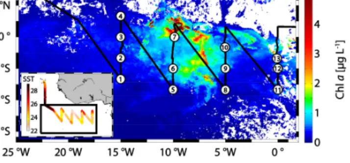
Cruise MSM18/3 onboard the RV Maria S. Merian took place from June 21 to July 21 2011. One goal of the cam- paign was the characterization of the Atlantic equatorial upwelling with regard to halocarbon emissions and their sources. RV Maria S. Merian started in Mindelo (Sao Vi- cente, Cape Verde) at 16.9^◦N and 25.0^◦W, and finished in Libreville (Gabon) at 0.4^◦N and 13.4^◦E with several transects across the equator. The ship entered the ACT several times. Measurements of halocarbons and phytoplankton pigments were conducted in surface water along the cruise track, and at 13 stations (Fig. 1). Samples for dissolved halocarbons from sea surface water were taken from a continuously work- ing pump in the ships moon pool at a depth of about 6.5 m every 3 h. Deep water samples were taken from up to eight different depths per station between 10 and 700 m from 12 L Niskin bottles attached to a 24-bottle-rosette with a CTD (conductivity temperature depth). Halocarbon stations 1–4 were located at the first meridional transect across the ACT at 15^◦W, stations 5–7 at the second transect at 10^◦W, 8–10 were located at the third section at around 5^◦W, and the last three stations 11–13 were taken during the last section at 0^◦E (Fig. 1). Water temperature and salinity were recorded with a thermosalinograph. Air pressure and wind speed were derived from sensors in 30 m height, averaged in 10 min inter- vals, and wind speed was corrected to 10 m. Global radiation was measured onboard in 19.5 m height with sensors (SMS-1 combined system from MesSen Nord, Germany) measuring downward incoming global radiation (GS, shortwave) and in- frared radiation (IR, long wave).

2.1 Sampling and analysis of halocarbons in seawater A purge and trap system attached to a gas chromatograph with mass spectrometric detection (GC-MS) in single ion mode was used to analyse 50 mL water samples for dissolved halocarbons. Volumetrically prepared standards in methanol were used for quantification. Precision lay within 3 % for CHBr₃, 6 % for CH₂Br₂, 15 % for CH₃I and 20 % for CH₂I₂ determined from duplicates. For a detailed description see Hepach et al. (2014).

(3)

Figure 1. Cruise track with SST in^◦C (small box) and the section (large box) where halocarbons were sampled in both the sea surface and during CTD stations (numbered circles), plotted on monthly average Chlafor July 2011 derived from mapped level 3 MODIS Aqua Data.

2.2 Phytoplankton pigment analysis and continuous measurement of chlorophylla

Water samples were filtered onto GF/F filters, shock-frozen in liquid nitrogen and stored at−80^◦C. Pigments listed in Table 1 of Taylor et al. (2011) were analysed using a HPLC technique according to Barlow et al. (1997) as described in Taylor et al. (2011). Surface pigment data were already used in a study by Bracher et al. (2015). All pigment data are already published and available from PANGAEA (http://doi.

pangaea.de/10.1594/PANGAEA.848586). For interpretation of the pigment data, CHEMTAX^®(Mackey et al., 1996) was used, and initiated with the pigment ratio matrix proposed by Veldhuis and Kraay (2004) for the subtropical Atlantic Ocean. The following phytoplankton groups were evaluated:

diatoms, Synechococcus-type, Prochlorococcus HL (high- light adapted) and Prochlorococcus LL (low-light adapted), dinoflagellates, haptophytes, pelagophytes, cryptophytes and prasinophytes.

Ten minute-averaged continuous surface maximum fluorescence measured by a microFlu-chl fluorometer from TriOS located in the ships moon pool was used to derive continuous total Chl a (T Chla)concentrations along the underway transect. This is based on the assumption that ac- tive fluorescence F is correlated to the amount of available T Chla(Kolber and Falkowski, 1993). The method to con- vert fluorescence to T Chla is described in detail in Tay- lor et al. (2011). Mean conversion factors specific for each zone were determined for collocated F and HPLC-T Chla (the sum of monovinyl Chl a, divinyl Chl a and Chloro- phyllide a; the latter is mainly formed as artefact of the former two during the extraction process and therefore included in the calculation) measurements. A linear regression ofr=0.83 (p< 0.01,n=89) was observed between surface HPLC-derivedT Chla and F-derivedT Chla, which indicates the robustness of the conversion of F to T Chla. The high depth resolved chlorophyll profiles were derived from fluorescence values obtained from a Dr. Haardt fluorometer

mounted to the CTD and calibrated with collocated HPLC- derivedT Chla concentrations at six depths of each profile according to Fujiki et al. (2011).

2.3 Correlation analysis of halocarbons

Different parameters were correlated to surface water halocarbons. Physical influences were investigated with 10 min averages of sea surface temperature (SST), sea surface salinity (SSS), global radiation and wind speed, and a relationship with location was explored using latitude. Biological parameters used for correlations wereT Chla, and the abundance of all phytoplankton groups. Since most of the data sets were not normally distributed and common transformations into normal distributions were not possible, the Spearman’s rank correlation coefficientrs was applied. All correlations with p< 0.05 were regarded as significant.

Correlation analysis of the entire depth profile data set using the Spearman’s rank coefficient did not allow for draw- ing specific conclusions due to the complexity of the data set. Hence, the mixed influences on water column halocarbon concentrations were examined with principal component analysis (PCA) using MATLAB^®. PCA analyses the collec- tive variance of a data set including several variables. The PCA has the advantage to simplify a complex data set and find similarities. Concentrations of all four halocarbons, all phytoplankton groups, theT Chla, density, temperature, and salinity were included.

2.4 Mixed layer depth

Mixed layer depthszML were determined using the method introduced by Kara et al. (2000). It proved to be closest to the visually determinedz_ML from the temperature, salinity and density profiles. The mixed layer of each CTD profile was calculated as the depth where the temperature from the reference depth in the upper well-mixed temperature region was reduced by a threshold value of 0.8^◦C.

2.5 Calculation of sea-to-air fluxes of halocarbons The air-sea gas exchange parameterization of Nightingale et al. (2000) was applied to calculate sea-to-air fluxesFas of halocarbons (Eq. 1). Schmidt number corrections as reported by Quack and Wallace (2003) were applied to determine the compound-specific transfer coefficient kw. The air-sea concentration gradient was computed from sea surface water measurements and mean atmospheric mixing ratiosc_atm of 2.50 ppt for CHBr₃, 1.20 ppt for CH₂Br₂, and 0.50 ppt for CH₃I determined from 10 atmospheric data points during MSM18/3, and atmospheric mixing ratios of 0.01 ppt for CH₂I₂as reported by Jones et al. (2010) for the tropical At- lantic. Henry’s law constants H of Moore and co-workers (Moore et al., 1995a, b) were used to obtain the equilibrium

(4)

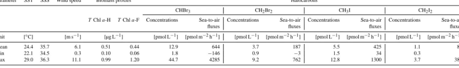
Table 1. Mean (minimum – maximum) values of physical parameters (sea surface temperature (SST), sea surface salinity (SSS), and wind speed), surface biomass proxies (T Chla-H:T Chlafrom HPLC measurements,T Chla-F:T Chladetermined from the continuously measuring fluorescence sensor), and sea surface concentrations, as well as sea-to-air fluxes of the four halocarbons CHBr₃, CH₂Br₂, CH₃I, and CH₂I₂during the cruise MSM18/3.

Parameter SST SSS Wind speed Biomass proxies Halocarbons

CHBr3 CH2Br2 CH3I CH2I2

TChla-H TChla-F Concentrations Sea-to-air Concentrations Sea-to-air Concentrations Sea-to-air Concentrations Sea-to-air

fluxes fluxes fluxes fluxes

Unit [^◦C] [m s⁻¹] [µg L⁻¹] [pmol L⁻¹] [pmol m⁻²h⁻¹] [pmol L⁻¹] [pmol m⁻²h⁻¹] [pmol L⁻¹] [pmol m⁻²h⁻¹] [pmol L⁻¹] [pmol m⁻²h⁻¹]

Mean 24.4 35.7 6.1 0.51 0.44 12.9 644 3.7 187 5.5 425 1.1 82

Min 22.1 34.5 0.3 0.10 0.06 1.8 −146 0.9 −3 1.5 34 0.3 3

Max 29.0 36.3 11.1 0.99 1.20 44.7 4285 9.2 762 12.8 1300 3.7 382

concentrationsc_atm/H.

F_as=k_w·

c_w−catm

H

. (1)

2.6 Calculation of diapycnal fluxes of halocarbons To estimate the halocarbon transport perpendicular to the stratification, Eq. (2) was used withFdiaas the diapycnal flux in mol m⁻²s⁻¹,ρas the seawater density in kg m⁻³,1cbe- ing the diapycnal gradient of the concentration in mol kg⁻¹, andKdiaas the diapycnal diffusion coefficient in m²s⁻¹.

Fdia=ρ·Kdia·1c. (2)

In the equatorial near surface water, molecular and double diffusion are negligible compared to turbulent mixing. Kdia

from turbulent mixing can be estimated from measurements of the velocity microstructure (turbulent motions on length scales of centimetres to metres). During MSM18/3, velocity microstructure profiling was performed immediately before or after taking halocarbon profiles, so that local and point- wise in time estimates of the diapycnal flux resulted from the combination of the two profiles via equation 2. The microstructure profiler (MSS) was a loosely tethered MSS90 equipped with airfoil shear probes, manufactured by Sea &

Sun Technology. In order to calculateK_diafrom velocity fluc- tuations measured by the MSS, first the average spectrum of vertical shear for a depth interval of typically 10 to 50 m was calculated and integrated to get an estimate of the average dissipation rate of turbulent kinetic energy (epsilon in W kg⁻¹). Equation (3), first proposed by Osborn (1980) al- lows to deduceKdia, withγ a function of the mixing effi- ciency andN the buoyancy frequency for the chosen depth interval.

Kdia=γ· ε

N². (3)

γ was chosen to be 0.2 following Hummels et al. (2013) for the tropical Atlantic. A more detailed description of the method to deriveK_diaand diapycnal fluxes below the mixed layer can be found in Schafstall et al. (2010), Hummels et al. (2013), and Schlundt et al. (2014).

3 Physical and biological characteristics of the investigation area

3.1 Oceanographic description

The equatorial Atlantic is described by a complex current system. The surface is characterized by the westward South Equatorial Current (SEC), which spreads between 3^◦N and 15^◦S and reaches as deep as 100 m, but has shallow mixed layers close to the equator (Tomczak and Godfrey, 2005).

The Equatorial Undercurrent (EUC) can be found below the SEC (Molinari, 1982), and is a narrow band between 2^◦N and 2^◦S flowing towards the east while reducing speed. It carries mostly water with characteristics of deeper tropical surface water (TSW) and of shallower central water. TSW around and north of the equator is characterized by high temperatures and comparably low salinities due to enhanced pre- cipitation (Tsuchiya et al., 1992). While the core of the EUC in the west is at 100 m, its position in the east follows the seasonal vertical migration of the thermocline (Stramma and Schott, 1999). In agreement with this, the mixed layer depth was shallow and ranged only between surface and 49 m with a mean of 28 m during MSM18/3. The mixed layer was also exposed to diurnal variability. During daytime, it was shallower due to warmer air temperatures and more stratification. At night, when the air temperature and SSTs cool, water mixes further down. The shallowest mixed layers were found between 0^◦N and 3^◦S in agreement with the location of the EUC. The Atlantic Cold Tongue (ACT) is a known feature in the equatorial region where SSTs between 20 and 5^◦W can drop by 5–7^◦C during May to September (Weingartner and Weisberg, 1991). Many uncertainties remain with respect to the exact mechanisms that lead to the development of the ACT. Jouanno et al. (2011) suggested that the strong increase of the westward SEC associated with the ITCZ (Philander and Pacanowski, 1986), and the maximum shear above the core of the underlying EUC lead to the low SSTs, confirmed later by microstructure measurements (Hummels et al., 2013;

Schlundt et al., 2014). Although the shear is maximal at 0^◦E, maximum cooling appears at 10^◦W due to the stronger stratification in the eastern basin of the equatorial Atlantic. SSTs during MSM18/3 of mean (range) 24.4 (22.1–29.0)^◦C and

(5)

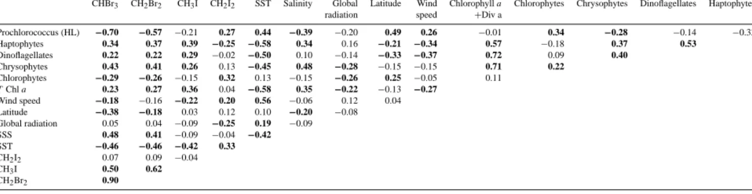
Table 2. Spearman’s rank correlation coefficientsrsof halocarbons with different physical parameters and phytoplankton species measured in surface water. Numbers printed in bold are regarded as significant withp< 0.05.

CHBr₃ CH₂Br₂ CH₃I CH₂I₂ SST Salinity Global Latitude Wind Chlorophylla Chlorophytes Chrysophytes Dinoflagellates Haptophytes

radiation speed +Div a

Prochlorococcus (HL) −0.70 −0.57 −0.21 0.27 0.44 −0.39 −0.20 0.49 0.26 −0.01 0.34 −0.28 −0.14 −0.33

Haptophytes 0.34 0.37 0.39 −0.25 −0.58 0.34 0.16 −0.21 −0.34 0.57 −0.18 0.37 0.53

Dinoflagellates 0.22 0.22 0.29 −0.02 −0.50 0.10 −0.14 −0.33 −0.37 0.72 0.09 0.40

Chrysophytes 0.43 0.41 0.26 0.13 −0.45 0.48 −0.28 −0.15 −0.15 0.71 0.22

Chlorophytes −0.29 −0.26 −0.15 0.32 0.13 −0.15 −0.26 0.25 −0.05 0.11

TChla 0.23 0.27 0.36 0.04 −0.58 0.35 −0.22 −0.13 −0.27

Wind speed −0.18 −0.16 −0.22 0.20 0.56 −0.06 0.12 0.04

Latitude −0.38 −0.18 0.03 0.12 0.10 −0.20 −0.08

Global radiation 0.05 0.04 −0.09 −0.25 0.19 −0.09

SSS 0.48 0.41 −0.09 −0.04 −0.42 SST −0.46 −0.46 −0.42 0.33 CH₂I₂ 0.07 0.09 −0.04

CH₃I 0.50 0.62

CH₂Br₂ 0.90

SSSs of 35.7 (34.5–36.3) were measured in the investigated region (Table 1, Fig. 2). Generally, high SSTs and low SSSs of less than 35.5 in the TSW were observed north of the equator. Lower SSTs and higher SSSs were measured in the south except for the 10^◦W section where these low SSTs and high SSSs were also found north of the equator. Maximum SSTs around the equator of 28.5^◦C were found at 3^◦N and 20^◦W, while the lowest SSTs of 22.1^◦C were located at 1^◦N and 10^◦W (Figs. 1, 2, Table 1).

3.2 Biological description

The cooling of SSTs in the ACT region is usually accom- panied by a phytoplankton bloom. Grodsky et al. (2008) found a seasonal peak of T Chla of 0.60 µg L⁻¹ in boreal summer. In comparison, surface T Chla during MSM18/3 reached values as high as 1.20 µg L⁻¹ around 0.8^◦N and 0^◦E (Fig. 2c). Very high T Chl a concentrations above 1.00 µg L⁻¹were also measured from the continuous fluorescence sensor around 10^◦W, coincidentally with the most intense cooling. The three hourly HPLC measurements of up to 0.99 µg L⁻¹generally also agree with the highT Chlamax- imum values measured with the fluorescence sensor (Fig. 2, Table 1). Additionally, nitrate and phosphate were significantly anticorrelated with SST (not shown), hence the up- welled water of the EUC was connected to enhanced biological production.

The most abundant phytoplankton group in the ACT were chrysophytes in both surface water and depth profiles dur- ing MSM18/3 (Fig. 2a). Chrysophytes, golden algae with flagellar hairs, are thought to be mostly common in fresh- water (Round, 1986). Nevertheless, they have been previ- ously shown to be also the most abundant phytoplankton group in several regions of the Atlantic ocean, including the lower latitudes around the equator (Kirkham et al., 2011).

This group correlated significantly with SST (r_s= −0.45) and SSS (r_s=0.48; Table 2), it hence seems to be associated with the upwelling water of the EUC. In the surface water, chlorophytes and Prochlorococcus HL correlated pos- itively with SST (r_s=0.13, not significant, and r_s=0.44,

significant) and negatively with SSS (r_s= −0.15, not significant, andr_s= −0.39, significant). They were associated with warmer and less salty water masses than chrysophytes, dinoflagellates and haptophytes. Thus, they were found pre- dominantly north of the equator. Prochlorococcus HL dom- inate among the species occurring from the surface down to 50 m. Prochlorococcus LL, only observed in deeper lay- ers (not shown here), were the most abundant group from about 75 m downwards in the water column. These results are in agreement with Johnson et al. (2006), where it was shown that Prochlorococcus dominate in oligotrophic tropi- cal waters, especially where nutrient concentrations are low at high temperatures (between 15^◦S and 15^◦N of the At- lantic Ocean).

4 Results

4.1 Surface water

4.1.1 CHBr₃and CH₂Br₂

Large regional variations were observed for the bromocarbons, especially for CHBr₃in surface water of the tropical Atlantic with a mean of 12.9 (1.8–44.7) pmol L⁻¹, and of 3.7 (0.9–9.2) pmol L⁻¹for CH2Br2(Fig. 2, Table 1). Concentra- tions from the underway measurements and from the shallowest profile depths (< 10 m) were included in the evalua- tion of the surface water concentrations. The observed values are in agreement with data from the tropical oligotrophic At- lantic north of 16^◦N and the Mauritanian upwelling ranging between 1.0 and 43.6 for CHBr₃ and 0.6–9.4 pmol L⁻¹ for CH₂Br₂with the largest values close to the coast and the upwelling (Quack et al., 2007a; Carpenter et al., 2009; Hepach et al., 2014). Quack et al. (2004) observed lower CHBr₃ of 2.3 pmol L⁻¹and CH₂Br₂of 0.2 pmol L⁻¹at 10^◦N through the tropical Atlantic in boreal fall and values of 12.8 and 5.3 pmol L⁻¹for CHBr₃and CH₂Br₂at the equator in agreement with our study. Values of up to 10 pmol L⁻¹(CHBr₃) and 3 pmol L⁻¹(CH₂Br₂)near the equator were reported by

(6)

Figure 2. (a) Species composition (HL – high light, LL – low light), (b) SST and salinity during the cruise, (c)T Chlafrom underway fluorescence sensor measurements and global radiation, (e) CHBr₃and CH₂Br₂in surface sea water, and (e) CH₃I and CH₂I₂surface sea water concentrations. The top numbers mark the CTD stations.

Liu et al. (2013b). The latter study covers the region during October and November, indicating that the equatorial Atlantic seems to be a larger source for bromocarbons during the intense cooling in the summer months. Both compounds show the same pattern in surface water throughout the MSM18/3 cruise with hot spots slightly south of the equator.

The very good correlation between CHBr₃and CH₂Br₂is in agreement with studies from several regions, mostly attributed to related sources for both compounds from macro- and microalgae (Nightingale et al., 1995; Moore et al., 1996;

Schall et al., 1997; Laturnus, 2001; Quack et al., 2007b;

Karlsson et al., 2008). Significant correlations to SST, SSS andT Chlawere found for CHBr3and CH2Br2, while very low insignificant correlations were observed with the 10 min averaged global radiation values (Table 2). The strongest cor- relations were found to Prochlorococcus HL withrs= −0.70 for CHBr3and−0.57 for CH2Br2, and to chrysophytes with rs=0.43, andrs =0.41, respectively.

4.1.2 CH3I and CH2I2

The second highest mean sea surface water concentration was observed for CH₃I of 5.5 (1.5–12.8) pmol L⁻¹ (Fig. 2, Table 1), which is in the range of earlier studies. These studies were widely spread in the region from 20^◦S to 25^◦N between the coasts of South America and Africa with values between 0 and 36.5 pmol L⁻¹ (Happell and Wallace, 1996;

Schall et al., 1997; Richter and Wallace, 2004; Jones et al., 2010; Hepach et al., 2014). 7.1 to 16.4 pmol L⁻¹were de- tected in the vicinity of our investigated region (Richter and Wallace, 2004). CH₂I₂was characterized by the lowest sea surface water concentrations of 1.1 (0.3–3.7) pmol L⁻¹during MSM18/3. Literature reports of CH₂I₂in the tropical At- lantic are very sparse: Schall et al. (1997) report on average three times higher values of 3.4 (2.1–6.8) pmol L⁻¹ in the tropical Atlantic, while Jones et al. (2010) measured a five times higher mean of 5.8 (0.9 and 17.1) pmol L⁻¹(reported in Ziska et al., 2013) in the northern tropical Atlantic.

(7)

Table 3. Concentrations of CHBr₃, CH₂Br₂andT Chla(from HPLC measurements) averaged over different depths at every CTD station (1–13), as well as the mixed layer depth. If a range is not given, only one measurement point exists. Bold numbers indicate the depth of maximum concentrations at this station.

0–30 m 31–60 m 61–100 m

zML Concentrations TChla Concentrations TChla Concentrations TChla

[m] [pmol L⁻¹] [µg L⁻1] [pmol L⁻¹] [µg L⁻¹] [pmol L¹] [µg L⁻¹]

CHBr3 CH2Br2 CHBr3 CH2Br2 CHBr3 CH2Br2

1 34 5.4

(3.2–6.5)

1.7 (1.3–2.1)

0.60 (0.52–0.69)

5.8 (3.7−7.9)

3.0 (1.8−4.2)

0.59 (0.53–0.65)

2.1 1.1 –

2 16 30.2

(25.4−35.0) 6.5 (6.4−6.6)

0.92 (0.76–1.07)

9.0 (7.6–10.3)

5.2 (5.1–5.4)

0.86 (0.74–0.97)

2.4 (1.2–4.6)

1.8 (0.8–3.6)

0.20 (0.10–0.30)

3 37 6.8

(6.2−7.4)

3.9 (3.6−4.2)

0.80 (0.75–0.86)

3.0 (2.6–3.2)

2.4 (2.4–2.5)

0.65 (0.51–0.80)

2.3 (2.2–2.5)

2.3 (2.3–2.3)

0.18

4 14 12.5

(5.8−19.2) 7.2 (3.8−10.6)

0.56 (0.26–0.86)

5.9 (4.8–6.9)

3.1 (3.0–3.2)

0.80 (0.79–0.81)

2.6 (2.0–3.2)

2.5 (1.8–3.2)

0.19 (0.13–0.26)

5 49 14.0

(13.6−14.4) 4.2 (4.0–4.3)

0.34 (0.28–0.39)

11.7 4.8 0.58 7.6

(6.6–8.5) 7.4 (6.1−8.6)

0.39 (0.24–0.53)

6 12 13.4

(12.5−14.3) 5.0 (3.8−6.3)

0.99 5.4

(5.1–5.7) 4.8 (4.7–4.8)

0.30 (0.17–0.43)

4.9 (4.7–5.1)

4.6 (4.6–4.7)

0.10 (0.04–0.17)

7 – 11.2

(8.8−13.7) 4.6 (3.5−4.6)

0.71 (0.65–0.76)

3.7 (2.5–4.9)

3.4 (2.5–4.2)

0.46 (0.44–0.48)

3.1 (2.9–3.4)

3.0 (2.9–3.1)

0.11 (0.06–0.17)

8 45 5.0

(4.7–5.3)

1.0 (0.6–1.4)

0.34 (0.31–0.38)

7.0 (5.7−8.3)

2.5 (1.9−3.2)

0.51 (0.47–0.58)

1.1 1.5 0.51

9 21 3.6

(2.7–4.5)

1.8 (1.6–2.0)

0.75 (0.64–0.85)

8.9 (7.4−10.3)

4.2 (3.9−4.6)

0.77 (0.68–0.85)

5.4 (4.5–6.3)

3.2 (2.6–3.7)

0.24 (0.17–0.32)

10 10 5.2

(4.9–5.5)

2.6 (2.3–2.8)

0.50 (0.41–0.59)

8.9 (8.3−9.5)

3.8 (3.7−4.0)

0.62 (0.51–0.73)

3.5 (3.1–3.9)

2.5 (2.4–2.6)

0.47 (0.32–0.62)

11 24 6.0

(4.1–7.9)

2.5 (1.8–3.3)

0.46 (0.42–0.49)

13.1 4.3 0.82 4.0

(2.5–6.8) 4.0 (2.8−6.0)

0.23 (0.04–0.44)

12 35 18.1

(16.4−19.8) 5.8 (5.6−6.1)

0.77 (0.76–0.79)

11.6 (9.1–14.1)

6.3 (5.4–7.1)

0.70 (0.68–0.72)

5.3 (4.7–6.0)

5.5 (5.3–5.8)

0.25

13 41 11.6

(6.9−16.4) 3.5 (2.5–4.4)

0.55 (0.51–0.58)

8.9 (8.3–9.5)

4.6 (3.0–5.6)

0.16 (0–0.48)

5.9 (3.3–7.6)

5.2 (4.1−5.7)

0.12 (0–0.30)

Similar to CHBr₃and CH₂Br₂sea surface CH₃I was significantly anticorrelated with SST (r_s= −0.42) and not correlated with global radiation (Table 2). In contrast to the bromocarbons, correlations were neither found to SSS, nor to latitude. Additionally, sea surface CH3I correlated to biomass indicators (T Chl a: rs=0.36). The regional distribution of CH3I often followed qualitatively that of haptophytes (r_s=0.39) with the most elevated concentrations south of the equator. Positive correlations were also found to dinoflagel- lates (r_s=0.29) and chrysophytes (r_s=0.26). A weak, but significant anticorrelation was observed to wind speed (r_s=

−0.22). In contrast to the other three halocarbons, CH₂I₂ was positively correlated with SST (r_s=0.33), and elevated concentrations were observed mostly north of the equator. A weak negative correlation of CH₂I₂ was found with global radiation (r_s= −0.25), indicating higher sea surface CH₂I₂ during the night time and lower concentrations during the day. CH2I2correlated both with chlorophytes (rs=0.32) and Prochlorococcus HL (rs=0.27).

4.2 Water column 4.2.1 CHBr3and CH2Br2

CHBr₃ and CH₂Br₂ showed maxima at the surface, in the mixed layer and below it (Fig. 3, Table 3). The highest deep maximum concentrations of both CHBr₃ (up to 19.2 pmol L⁻¹)and CH₂Br₂(up to 10.6 pmol L⁻¹)were observed in profile 4. At stations where CHBr₃ was most elevated at the surface (profiles 2, 7, 12, 13), much higher overall CHBr₃ concentrations of up to 35.0 pmol L⁻¹ were

measured. CH₂Br₂ only reached maximum values of up to 6.6 pmol L⁻¹in the surface (profiles 2, 7).

In contrast to surface water, CHBr3and CH2Br2were distributed differently in the water column with CH2Br2being elevated 10 m below CHBr3in several profiles (Fig. 3e). This can also be seen in the T-S diagrams of these compounds (Fig. 4a, b): while the most elevated CHBr3was observed in the density layers between 1024 and 1025 kg m⁻³(shallower central water of the EUC), CH₂Br₂was often also elevated in the denser, deeper layers below 30 m (Table 3). The maxima of both compounds were mostly in the vicinity of the T Chla maximum. Results of the PCA (Fig. 5) also show the dissimilarity of CHBr₃and CH₂Br₂ at depth: while the variance of CHBr₃seems comparable to salinity and several phytoplankton groups such as chrysophytes, CH₂Br₂shows many similarities with the distribution of CH₂I₂in the water column.

4.2.2 CH3I and CH2I2

In agreement with CHBr3and CH2Br2, CH3I was elevated in the surface (three profiles 4, 6, 7; Table 4, Fig. 3b) with values of up to 12.8 pmol L⁻¹, and also elevated in the deeper layers in and below the mixed layer (Fig. 3f), reaching up to 8.5 pmol L⁻¹. Most maxima of CH₃I were observed closer to the surface within the mixed layer (Fig. 4d). The PCA of CH₃I revealed that its variance was similar to the variance of dinoflagellates and temperature (Fig. 5).

CH₂I₂ was always depleted in the surface. Maxima of CH₂I₂were found in different depths, sometimes associated with theT Chlamaximum (Fig. 3f), and mostly below the

(8)

00 55 1010 1515

100 100 75 75 50 50 25 25

00 00 55 1010 1515

1022

1022 10241024 10261026 10281028 34.6

34.6 35.235.2 35.835.8 36.436.4

10

10 1717 2424 3131

100 100 75 75 50 50 25 25 00

Halocarbons [pmol L

Halocarbons [pmol L^-1^-1]] Temperature [°C]Temperature [°C]

Density [kg m Density [kg m^-3^-3]]

Depth [m]Depth [m]

CHBr CHBr₃₃ CH CH₂₂BrBr₂₂ CH CH₃₃II CH CH₂₂II₂₂ Temperature Temperature Salinity Salinity Density Density TChl TChl aa

Mixed layer depth Mixed layer depth 00 0.20.2 0.40.4 0.60.6

Salinity Salinity

TChl TChl aa [µg L [µg L^-1^-1]]

a) a)

e) e)

i)i)

b)

b) c)c) d)d)

f)

f) g)g) h)h)

j)j) k)k) l)l)

Figure 3. Selected CTD profiles (top – down: profiles 7, 9 and 10, see Fig. 1 for the location) of CHBr₃, CH₂Br₂, CH₃I, and CH₂I₂in (a–b, e–f), and (i–j), along with temperature, salinity, and density (c, g, k), as well asT Chlain (d), (h), and (l), and the mixed layer depth as black dashed line at the same stations.

10 20

30 ₂₂ ₂₃

24 25 26 27

28 0

20

40 ²² ²³₂₄

25 26 27

28 0

5 10

22 23

24 25 26 27

28 0

5 10

22 23

24 25 26 27

28 0

5 10 15

35 36

22 23

24 25 26 27

28 0

0.2 0.4

35 36

22 23

24 25 26 27

28 0

0.2 0.4

a) CHBr₃ b) CH₂Br₂

d) CH₃I

c) CH₂I₂

Theta [°C]

Salinity

e) Chrysophytes f) Prochlorococcus LL

35 36 10

20 30

Figure 4. (a–d) Temperature–Salinity (T–S) plots for halocarbons (in pmol L⁻¹)and (e–f) phytoplankton species (in µg ChlaL⁻¹). Square markers indicate surface values of halocarbons from underway measurements, circles are depth measurements from CTD profile, and the lines indicate the potential density – 1000.

mixed layer (Fig. 3j). The maxima in deeper depths appeared concurrently with the deeper CH₂Br₂maxima (Fig. 4), which is also expressed in the PCA (Fig. 5). Values were generally much higher in deeper depths with e.g. 13.8 pmol L⁻¹ between 60 and 100 m at profile 5. The highest concentrations of the whole cruise of 16.0 pmol L⁻¹(profile 1) were found between 30 and 60 m. Concentrations of only up to 12.0 pmol L⁻¹ were found between 0 and 30 m (profile 6;

Table 4).

4.3 Fluxes

4.3.1 CHBr₃and CH₂Br₂

Sea-to-air fluxes of CHBr₃ and CH₂Br₂ of 644 (−146–

4285) and 187 (−3–762) pmol m⁻²h⁻¹ during MSM18/3 were larger during the first two western NS-transects of the cruise which were characterized by higher seawater concentrations, as well as higher wind speeds (Table 1, Fig. 6). Car- penter et al. (2009) and Hepach et al. (2014) reported−150

(9)

−0.5

−0.5 −0.4−0.4 −0.3−0.3 −0.2−0.2 −0.1−0.1 00 0.10.1 0.20.2 0.30.3 0.40.4 0.50.5

−0.5

−0.4

−0.3

−0.2

−0.1

−0.1 00 0.1 0.1 0.2 0.2 0.3 0.3 0.4 0.4 0.5 0.5

CH CH₂₂BrBr₂₂

CHBr CHBr₃₃ CH

CH₂₂II₂₂

Temperature Temperature Salinity

Salinity Density

Density

Diatoms Diatoms

Synechococccus Synechococccus

Prochlorococcus HL Prochlorococcus HL Prochlorococcus LL

Prochlorococcus LL

Dinoflagellates Dinoflagellates Haptophytes Haptophytes Chrysophytes Chrysophytes Chlorophytes Chlorophytes

Cryptophytes Cryptophytes

Prasinophytes Prasinophytes

Chl Chl aa + Div + Div aa

Component 1 (44.6 %) Component 1 (44.6 %)

Component 2 (13.8 %) Component 2 (13.8 %)

CH CH₃₃II

Figure 5. Principal component analysis (PCA) of halocarbon and phytoplankton species composition data, as well as temperature, salinity, and density for the 13 CTD stations during MSM18/3.

Table 4. Concentrations of CH₃I, CH₂I₂and the sum ofT Chlaaveraged over different depths at every CTD station (1–13), as well as the mixed layer depth. If a range is not given, only one measurement point exists. Bold numbers indicate the depth of maximum concentrations at this station.

0–30 m 30–60 m 60–100 m

z_ML Concentrations TChla Concentrations TChla Concentrations TChla

[m] [pmol L⁻¹] [µg L⁻¹] [pmol L⁻¹] [µg L⁻¹] [pmol L⁻¹] [µg L⁻¹]

CH₃I CH₂I₂ CH₃I CH₂I₂ CH₃I CH₂I₂

1 34 2.7

(2.1−3.4) 4.5 (1.2–6.8)

0.60 (0.52–0.69)

2.5 (1.8–3.2)

9.9 (3.9−16.0)

0.59 (0.53–0.65)

0.2 1.7 –

2 16 2.8

(0.4–5.2)

4.8 (1.7–8.0)

0.92 (0.76–1.07)

3.1 (2.7−3.6)

12.2 (11.5−12.9)

0.86 (0.74–0.97)

0.6 (0.1–1.3)

2.0 (0.7–4.3)

0.20 (0.10–0.30)

3 37 8.5

(8.4−8.5) 4.1 (1.7–6.4)

0.80 (0.75–0.86)

2.6 (1.0–3.5)

4.6 (4.3−4.9)

0.65 (0.51–0.80)

0.7 (0.4–1.1)

3.3 (2.3–4.4)

0.18

4 14 6.1

(5.5−6.6)

7.0 0.56

(0.26–0.86)

4.6 (4.6–4.7)

2.3 (2.2–2.4)

0.80 (0.79–0.81)

0.8 (0.7–0.9)

1.0 (0.7–1.3)

0.19 (0.13–0.26)

5 49 5.4 0.6

(0.5–0.7)

0.34 (0.28–0.39)

4.5 4.9 0.58 2.4

(1.9–3.0) 10.5 (7.1−13.8)

0.39 (0.24 - 0.53)

6 12 10.4

(8.0−12.8) 6.9 (1.8−12.0)

0.99 1.6

(1.5–1.7) 4.0 (3.1–4.8)

0.30 (0.17–0.43)

1.4 (1.0–1.7)

2.4 (1.7–3.1)

0.10 (0.04–0.17)

7 – 4.1

(3.4−4.8) 2.3 (1.2–3.4)

0.71 (0.65–0.76)

1.3 (1.2–1.3)

4.7 (3.3−6.1)

0.46 (0.44–0.48)

0.9 (0.6–1.2)

2.0 (1.5–2.7)

0.11 (0.06–0.17)

8 45 0.2

(0.1–0.4)

0.3 (0.3–0.3)

0.34 (0.31–0.38)

4.7 (3.0−7.0)

1.2 (0.5–1.9)

0.51 (0.47–0.58)

0.0 2.4 0.51

9 21 4.4

(4.1–4.8)

1.3 (1.2–1.5)

0.75 (0.64–0.85)

5.3 (3.4−7.3)

6.2 (4.5−8.0)

0.77 (0.68–0.85)

1.3 (1.3–1.3)

2.9 (2.3–3.6)

0.24 (0.17–0.32)

10 10 4.5

(3.6–5.5)

0.5 (0.4–0.6)

0.50 (0.41–0.59)

4.9 (4.2−5.7)

1.3 (0.9–1.7)

0.62 (0.51–0.73)

0.8 (0.7–0.9)

3.4 (2.6−4.1)

0.47 (0.32–0.62)

11 24 3.8

(2.9−4.6)

0.4 0.46

(0.42–0.49)

4.4 2.3 0.82 1.7

(1.0–2.3) 1.7 (0.6−3.2)

0.23 (0.04–0.44)

12 35 7.0

(6.8−7.1) 1.2 (0.3–2.2)

0.77 (0.76–0.79)

2.7 4.1

(3.8−4.3)

0.70 (0.68–0.72)

2.0 2.7

(1.6–3.8)

0.25

13 41 5.1

(4.3−5.9) 1.5 (0.8–2.1)

0.55 (0.51–0.58)

3.8 (2.0–5.6)

5.9 (3.9−7.4)

0.16 (0–0.48)

1.0 (0.1–2.0)

3.4 (1.0–4.8)

0.12 (0–0.30)

and 3504 pmol m⁻²h⁻¹CHBr3fluxes as well as of 5–917 for CH2Br2from the Cape Verde and Mauritanian upwelling region. The lower fluxes in the equatorial region are a result of the lower wind speeds measured during MSM18/3, ranging from 0.3–11.1 with a mean of 6.1 m s⁻¹, and the lower concentration gradients in comparison to Carpenter et al. (2009).

Quack et al. (2004) reported CHBr₃fluxes from the equato-

rial Atlantic of 2700 (±800) pmol m⁻²h⁻¹, which compare well to this study.

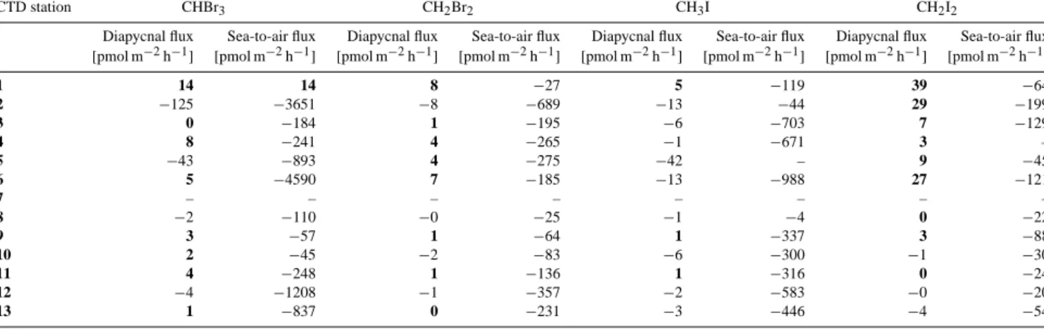
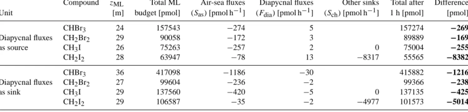
Diapycnal fluxes are the fluxes of halocarbons that diffuse out or into the mixed layer from below the thermocline. Max- ima within the mixed layer will lead to fluxes towards the thermocline, while maxima below the mixed layer will result in a flux of halocarbon-molecules into the mixed layer.

Diapycnal fluxes of halocarbons were generally low although