Supporting Information for ”Revisiting the Cause of the Eastern Equatorial Atlantic Cold Event in 2009”

JOURNAL OF GEOPHYSICAL RESEARCH

Supporting Information for ”Revisiting the Cause of the Eastern Equatorial Atlantic Cold Event in 2009”

Kristin Burmeister,¹ Peter Brandt,^1,2 and Joke F. L¨ubbecke^1,2

Contents of this file

1. Figures S1 to S3

Introduction This supporting information provides additional figures, Figures S1-S2 to demonstrate that both reanalysis data sets simulate the 2009 cold event well and Figure S3 to visualize the relative importance of meridional velocity and temperature in the anomalous MTA in 2009.

Corresponding author: K. Burmeister, GEOMAR Helmholtz Centre for Ocean Research Kiel D¨usternbrooker Weg 20, D-24105 Kiel, Germany. (kburmeister@geomar.de)

1GEOMAR Helmholtz Centre for Ocean Research Kiel, Kiel, Germany

2Christian-Albrechts-Universit¨at zu Kiel, Kiel, Germany

D R A F T June 7, 2016, 2:27pm D R A F T

X - 2 BURMEISTER ET AL.: 2009 EQUATORIAL ATLANTIC COLD EVENT

25 m² s⁻² (i) TMI

10°S 0°N 10°N

50°W 40°W 30°W 20°W 10°W 0°E 10°E (a) May

25 m² s⁻²

(b) Jun 10°S

0°N 10°N

50°W 40°W 30°W 20°W 10°W 0°E 10°E 25 m² s⁻²

10°S 0°N 10°N

50°W 40°W 30°W 20°W 10°W 0°E 10°E (c) Aug

≤ −1.6 −1.2 −0.8 −0.4 0 0.4 0.8 1.2 ≥ 1.6 SST anomaly in °C

25 m² s⁻² (ii) GODAS

10°S 0°N 10°N

50°W 40°W 30°W 20°W 10°W 0°E 10°E (a) May

25 m² s⁻²

(b) Jun 10°S

0°N 10°N

50°W 40°W 30°W 20°W 10°W 0°E 10°E 25 m² s⁻²

10°S 0°N 10°N

50°W 40°W 30°W 20°W 10°W 0°E 10°E (c) Aug

≤ −1.6 −1.2 −0.8 −0.4 0 0.4 0.8 1.2 ≥ 1.6 SST anomaly in °C

25 m² s⁻² (iii) ORA−S4

10°S 0°N 10°N

50°W 40°W 30°W 20°W 10°W 0°E 10°E (a) May

25 m² s⁻²

(b) Jun 10°S

0°N 10°N

50°W 40°W 30°W 20°W 10°W 0°E 10°E 25 m² s⁻²

10°S 0°N 10°N

50°W 40°W 30°W 20°W 10°W 0°E 10°E (c) Aug

≤ −1.6 −1.2 −0.8 −0.4 0 0.4 0.8 1.2 ≥ 1.6 SST anomaly in °C

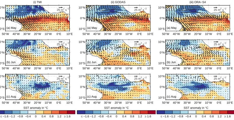
Figure S1. Anomalies of SST (shading) from (i) TMI satellite data, (ii) GODAS and (iii) ORA-S4 reanaylsis data and CCMP pseudo wind stress (arrows) with respect to the climatology mean (1998-2011) for (a) May, (b) June and (c) August 2009.

D R A F T June 7, 2016, 2:27pm D R A F T

BURMEISTER ET AL.: 2009 EQUATORIAL ATLANTIC COLD EVENT X - 3

(a) 4°N, 38°W

(i) PIRATA

50 100 150

≤ −5 −4 −3 −2 −1 0 1 2 3 4 ≥ 5

Temperature anomaly in °C (b) 4°N, 23°W

50 100 150

Depth in m (c) 0°N, 23°W

50 100 150

(d) 0°N, 10°W 50

100 150

Jan Feb Mar Apr May Jun Jul Aug Sep Oct Nov Dec (e) 0°N, 0°E

50 100 150

(a) 4°N, 38°W

(ii) GODAS

50 100 150

≤ −5 −4 −3 −2 −1 0 1 2 3 4 ≥ 5

Temperature anomaly in °C (b) 4°N, 23°W

50 100 150

Depth in m (c) 0°N, 23°W

50 100 150

(d) 0°N, 10°W 50

100 150

Jan Feb Mar Apr May Jun Jul Aug Sep Oct Nov Dec (e) 0°N, 0°E

50 100 150

(a) 4°N, 38°W

(iii) ORA−S4

50 100 150

≤ −5 −4 −3 −2 −1 0 1 2 3 4 ≥ 5

Temperature anomaly in °C (b) 4°N, 23°W

50 100 150

Depth in m (c) 0°N, 23°W

50 100 150

(d) 0°N, 10°W 50

100 150

Jan Feb Mar Apr May Jun Jul Aug Sep Oct Nov Dec (e) 0°N, 0°E

50 100 150

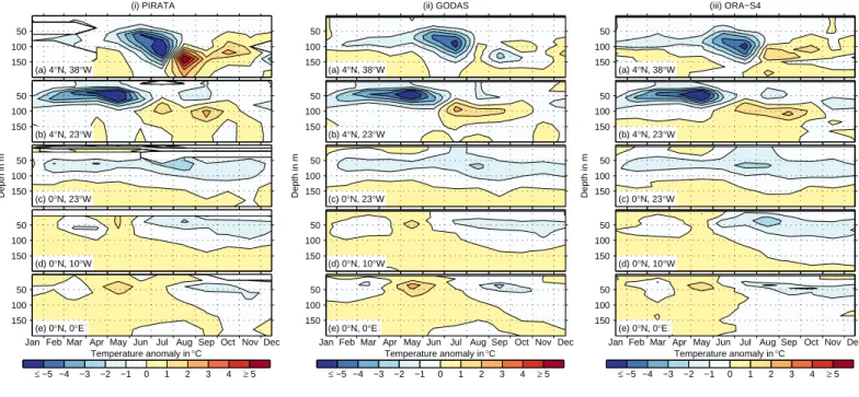
Figure S2. Monthly mean temperature anomalies from (i) PIRATA buoys data, (ii) GODAS and (iii) ORA-S4 reanalysis data with respect to the climatology mean (2006-2013) at different PIRATA bouy locations.

D R A F T June 7, 2016, 2:27pm D R A F T

X - 4 BURMEISTER ET AL.: 2009 EQUATORIAL ATLANTIC COLD EVENT

−1

−0.8

−0.6

−0.4

−0.2 0 0.2 0.4 0.6 0.8

°C/month

GODAS −<v> (dT/dy)′

Jan Feb Mar Apr May Jun Jul Aug Sep Oct Nov Dec 0−30m

30−60m 60−90m

−1

−0.8

−0.6

−0.4

−0.2 0 0.2 0.4 0.6 0.8

°C/month

ORA−S4 −<v> (dT/dy)′

Jan Feb Mar Apr May Jun Jul Aug Sep Oct Nov Dec 0−30m

30−60m 60−90m

−1

−0.8

−0.6

−0.4

−0.2 0 0.2 0.4 0.6 0.8

°C/month

GODAS −v′ <dT/dy>

Jan Feb Mar Apr May Jun Jul Aug Sep Oct Nov Dec 0−30m

30−60m 60−90m

−1

−0.8

−0.6

−0.4

−0.2 0 0.2 0.4 0.6 0.8

°C/month

ORA−S4 −<v> (dT/dy)′

Jan Feb Mar Apr May Jun Jul Aug Sep Oct Nov Dec 0−30m

30−60m 60−90m

−1

−0.8

−0.6

−0.4

−0.2 0 0.2 0.4 0.6 0.8

°C/month

GODAS −v′ (dT/dy)′

Jan Feb Mar Apr May Jun Jul Aug Sep Oct Nov Dec 0−30m

30−60m 60−90m

−1

−0.8

−0.6

−0.4

−0.2 0 0.2 0.4 0.6 0.8

°C/month

ORA−S4 −v′ (dT/dy)′

Jan Feb Mar Apr May Jun Jul Aug Sep Oct Nov Dec 0−30m

30−60m 60−90m

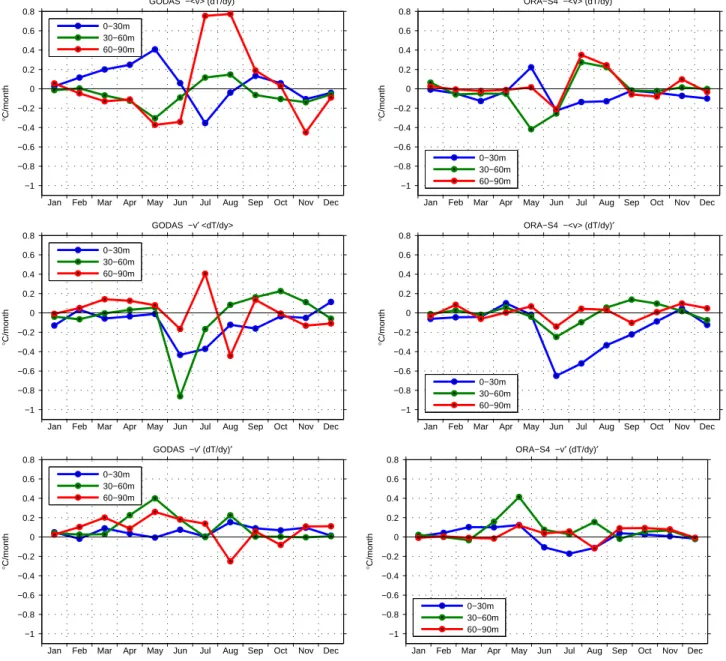
Figure S3. − < v > (dT /dy)^′ (upper), −v^′ < dT /dy > (middle) and −v^′(dT /dy)^′ (lower) of GODAS (left column) and ORA-S4 (right column) reanalysis data within 30^◦W - 15^◦W to 3^◦S - 3^◦N for three different depth ranges (0 m-30 m in blue, 30 m-60 m in green, 60 m-90 m in red). The <> denotes monthly mean seasonal cycle values (1980-2014) and the prime denotes 2009 monthly anomaly values with respect to the mean seasonal cycle. Note that positive values indicate a warming and negative values indicate a cooling by meridional advection.

D R A F T June 7, 2016, 2:27pm D R A F T