1 Geophysical Research Letters
Supporting Information for
Variability and trends in Southern Ocean eddy activity in 1/12° ocean model simulations
Lavinia Patara1, Claus W. Böning1, Arne Biastoch1
1 GEOMAR Helmholtz Centre for Ocean Research Kiel, Kiel, Germany
Contents of this file Text S1 to S3 Figures S1 to S5
Additional Supporting Information (Files uploaded separately)
Caption for Movies S1 to S2 Introduction
The supporting information contains a description of methodological aspects (Text S1 to S3), five figures (Figure S1 to S5) and two movies (Movie S1 to S2), which have been realized using the model outputs of ORCA025 and ORION12.
Text S1.
For technical reasons, a discontinuity is present in the nested domain of ORION12 between 69.5°E and 76.5°E (Fig. 1a). In the following we assess that this discontinuity does not have a significant effect on the mesoscale activity within and downstream of the discontinuity. First, we compare the sea surface height (SSH) variance (a measure of surface geostrophic eddy variability) in a standalone ORCA025 experiment at 1/4°
resolution with the SSH variance in the ORCA025 host model of the ORION12 configuration (Fig. 1d). Within the nest discontinuity, SSH variance in the host model of ORION12 is ~20% higher than in the standalone ORCA025 model, despite the fact that the two models have the same horizontal resolution in the nest discontinuity. This behavior may be explained by the capability of the “eddy-permitting” host model of ORION12 of maintaining much of the mesoscale activity formed in the nested domain
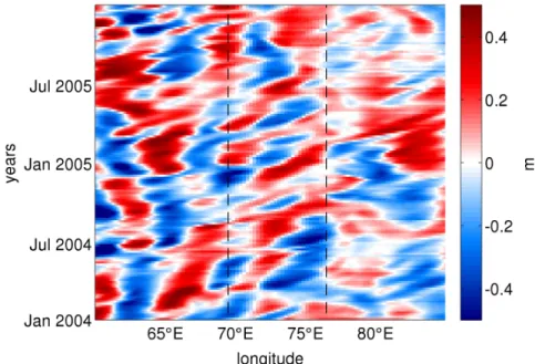
2 within the discontinuity (Movie S2). To further corroborate this deduction, a Hovmöller diagram of SSH anomalies at 44.5°S for longitudes embracing the nest discontinuity (Fig. S3) shows that SSH anomalies originating west of the nest discontinuity propagate without hindrance across the nest discontinuity, indicating that eddies formed in the nested domain are not dissipated within the host grid.
Text S2.
The ORCA025 model exhibits very little formation of Antarctic Bottom Water (AABW) on the continental shelf, as typical for this class of ocean models [Goosse et al., 2001;
Heuzé et al., 2013]. The progressive loss of dense AABW, a process that decreases the baroclinicity of the ACC on multi-decadal time scales, gives rise to a negative trend in the ACC transport (Fig. S1a). To achieve a better representation of AABW, we apply a three-dimensional relaxation sponge in areas of recently formed AABW (black regions outlined in Fig. S4) where we relax temperature and salinity to the World Ocean Atlas climatology [Levitus et al., 1998] with a relaxation time scale of one year. The sponge region is confined to water masses approximately south of the 0.5°C isotherm, defining the Southern ACC Front, and is restricted to a depth 1000 m below the surface and 500 m above the ocean bottom in order to avoid spurious sources of vorticity. The application of the three-dimensional relaxation sponge yields an attenuation of the model drift of the ACC transport of about 50% (Fig. S1a). Given that the relaxation is applied regionally, the concern could rise that the regionality of the EKE multi-decadal changes found in the HIND experiment might be affected by the regionality of the relaxation. This however does not appear to be the case: in the HIND experiment (detrended with the CLIM experiment as throughout this paper) residual trends in temperature and salinity in the AABW depth range do not have any spatial correspondence with the areas of relaxation (Fig. S4). This is likely because the relaxed water masses do not remain confined to the relaxation domains but circulate around the Antarctic continent.
Text S3.
Throughout this study we analyze EKE at 100 m depth. This diagnostic has the advantage of being based on the full ocean velocity fields and of being negligibly affected by both wind-induced velocities and interaction with the topography. In order to perform a clean comparison between simulated and satellite-observed EKE we also computed surface geostrophic velocities based on 5-day means of sea surface height (Fig. S5). It can be seen that overall the variability and correlations with the AVISO product are comparable when using surface geostrophic EKE or EKE at 100 m depth.
3 Figure S1. (a) Volume transport of the ACC at Drake Passage in two ORCA025 simulations using “normal year” forcing, one where relaxation to observed temperature and salinity was applied in the deep portions of the Weddell and Ross Seas (blue line), one without relaxation (red line), (b) EKE averaged over the ACC domain in the HIND experiment of ORION12, (c) volume transport of the ACC at Drake Passage in the HIND experiment of ORION12, (d) maximum residual meridional overturning circulation (MOC) in density space at 30°S in the HIND experiment of ORION12. For panels (b-d) blue lines indicate time series detrended with the linear fit of the CLIM experiment and red lines show undetrended time series. For all panels, thin lines and numbers indicate the linear trends of the resulting time series.
40 50 60 70 80
90 100 110 120
ACC transport in ORCA025
Sv
no relaxation AABW relaxation
a
−3.2 Sv decade−1
−1.7 Sv decade−1
1960 1970 1980 1990 2000 130
145 160
EKE in ORION12
cm2 sec−2
HIND HIND detrended with CLIM
b
2.7 cm2 sec−2 decade−1 5 cm2 sec−2 decade−1
1960 1970 1980 1990 2000 110
120 130
ACC transport in ORION12
Sv
c
HIND HIND detrended with CLIM
0.4 Sv decade−1 2 Sv decade−1
1960 1970 1980 1990 2000 10
15 20
Max MOC at 30°S in ORION12
Sv
HIND HIND detrended with CLIM
d
1.4 Sv decade−1 1 Sv decade−1
4 Figure S2. (a) Maximum correlations between EKE and regionally-averaged total wind stress (blue line), zonally-averaged total wind stress (red line), and the Southern Annular Mode (SAM) index (green line) in the temporal domain of 0 to 3 years lagging the wind stress (or the SAM index); the dashed line indicates the 95% confidence level, (b) temporal lag of the maximum correlation between wind stress and EKE (wind stress leading); lags shorter than 1 year are not resolved. The SAM index was computed as the difference between 41°S and 66°S of annually- and zonally-averaged sea level pressure in the COREv.2 data set. It should be noted that past studies have chiefly used the SAM index to infer a relationship between wind forcing and EKE [e.g. Meredith and Hogg, 2006; Morrow et al., 2010; Langlais et al., 2015].
5 Figure S3. Hovmöller diagram of sea surface height (SSH) anomalies at 44.5°S, i.e.
within the core of the ACC, for longitudes embracing the nest discontinuity. Shown are years 2004 and 2005. Dashed lines indicate the boundaries of the ORION12 nested domain. SSH anomalies are computed by removing the 2004-2005 SSH time-mean.
Figure S4. (a) Potential temperature and (b) salinity linear trends from year 1958 to 2007 in the HIND experiment (detrended with the CLIM experiment) computed over the AABW depth range, defined as depths for which potential density referenced to 4000 m (σ4) is higher than 1045.5 kg m-3. Only grid points south of the ACC (as defined in Fig.
2a) are shown. Black contours show areas of relaxed AABW properties below 1000 m depth.
6 Figure S5. Time series of EKE at 100 m depth in HIND (red line, from 1958 to 2007), of surface geostrophic EKE in HIND (blue line, from 1958 to 2007) and of surface geostrophic EKE in the AVISO satellite product (black line, from 1993 to 2007). Surface geostrophic velocities are computed based on 5-day means of simulated sea surface height in the model and of observed absolute dynamic topography in AVISO. Spatial averages are performed over (a) the whole ACC domain and over (b-f) sectors of the ACC (corresponding sector numbers are shown in Fig. 2c). The left y-axis refers to both EKE at 100 m and surface geostrophic EKE in HIND.
Movie S1. Animation showing Southern Ocean current speed at 100 m depth simulated by ORION12. Red (blue) areas indicate currents with high (low) velocities. The animation is based on 5-day means of the model output and covers the time span from 1 January 2001 to 31 December 2001.
Movie S2. Animation showing simulated ocean speed at 100 m depth in the Indian Ocean, in the vicinity of the discontinuity of the ORION12 nested domain (69.5°E- 76.5°E). Left: ORCA025 (global 1/4° ocean model), right: ORION12 (1/12° nest in the
7 ACC domain embedded within ORCA025); black lines show the nest contours. The fine and eddy-rich structure of the ACC flow is clearly visible in the 1/12° simulation.
Nevertheless, also ORCA025 is capable of producing and maintaining large eddies within the nest discontinuity. The animation is based on 5-day means of the model output and covers the time span from 1 January 2001 to 31 December 2001.
References:
Goosse, H., J.M. Campin, and B. Tartinville (2001), The sources of Antarctic bottom water in a global ice ocean model, Ocean Modelling, 3 (1-2), 51-65.
Heuzé, C., K.J. Heywood, D.P. Stevens, and J.K. Ridley (2013), Southern Ocean bottom water characteristics in CMIP5 models, Geophys. Res. Lett. 40, doi:10.1002/grl.50287.
Langlais, C. E., S. R. Rintoul, and J. D. Zika (2015), Sensitivity of Antarctic Circumpolar Current Transport and Eddy Activity to Wind Patterns in the Southern Ocean, J. Phys.
Oceanogr., 45 (4), 1051-1067, 10.1175/JPO-D-14-0053.1.
Levitus, S. et al. (1998), World Ocean Database 1998, vol. 1, Introduction, NOAA Atlas NESDIS, 18, NOAA, Silver Spring, Md.
Meredith, M. P., and A. M. Hogg (2006), Circumpolar response of Southern Ocean eddy activity to a change in the southern annular mode, Geophys. Res. Lett., 33, L16608, doi:10.1029/2006GL026499.
Morrow, R., M. L. Ward, A. M. Hogg, and S. Pasquet (2010), Eddy response to Southern Ocean climate modes, J. Geophys. Res., 115, C10030, doi:10.1029/2009JC005894.