1 Geophysical Research Letters
Supporting Information for
Southern Ocean deep convection as a driver of Antarctic warming events J.B. Pedro1,*, T. Martin2,*, E. J. Steig3, M. Jochum1, W. Park2, & S.O. Rasmussen1
1Center for Ice and Climate, Niels Bohr Institute, University of Copenhagen, Denmark
2GEOMAR Helmholtz Centre for Ocean Research Kiel, Kiel, Germany
3University of Washington, Seattle, WA, USA
*Corresponding authors with equal contributions to the study: jpedro@nbi.ku.dk, tomartin@geomar.de
Contents of this file
Supporting Figures S1 to S4 Supporting Table S1
Supporting References Introduction
The Supporting Figures and Table provide additional data from the Kiel Climate Model simulation used in the main text. References cited in the Supporting Figure captions are listed at the end.
2 Figure S1. Time series of: a) modeled annual mean mixed-layer depth over the
convection region (58–68˚S, 35˚W–10˚E); b) sea-surface temperature averaged over the convection region; c) Southern Ocean (SO) heat content of the Atlantic-Indian sector (70˚W–80˚E, 40˚–90˚S). Gray shading indicates periods without deep convection in the Weddell Sea. The blue arrow indicates SO heat loss during convection, the red arrow indicates SO heat storage after the convection event has ended. d) Map of cumulative ocean heat loss during a convective period, calculated as heat content difference of stage 2 minus stage 1 composites. Solid and dashed magenta outlines mark 200 m and 1000 m annual mean mixed layer depth during stage 1 indicating the convection region.
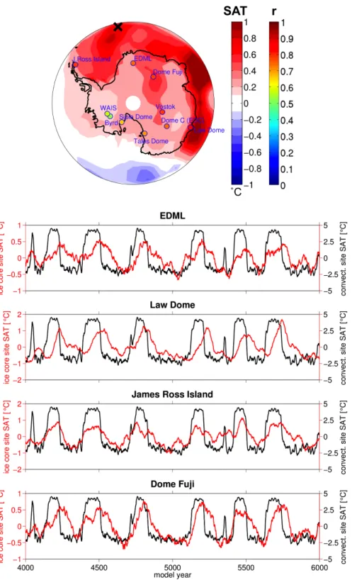
3 Figure S2. Map showing the surface-air-temperature (SAT) anomaly during stage 2 (cf.
Figure 3d). Circles mark locations of ice-core records. Color-coding of the circles depicts the maximum lagged correlation coefficient of modeled local SAT with SAT over the convection area (black cross in Weddell Sea). Lower panels show time series of
modeled SAT anomalies at selected ice-core sites (red) together with the SAT anomaly over the convection region (black). Note different y-axis scaling for red lines.
4
5 Figure S3. Composites of zonal mean anomalies for stage 1 (blue lines) and stage 2 (red lines) for just the Atlantic sector, 70˚W–30˚E (left panels) and for the circumpolar mean (right panels). a,b) Sea surface temperatures (SST). c,d) Westerly 10 m wind speed. e,f) Westerly 500-hPa wind speed. g,h) Sea-surface height (SSH). Bold gray lines depict the long-term mean westerly wind speed (u-component) at 10 m height (a–d) and at the 500 hPa level (e,f) as an indication for the location of the westerlies, and in (g,h) the long-term mean sea-surface height as a deviation from the global mean; see y-axis scaling on right.
In (g,h) the long-term mean location of the ACC is indicated by a black “bullseye”.
NGRIP 18 O (permil)
5.1
5.2 6 7 GI−8 9
10 11 GI−12 GI−14 15.2
16 17
a)
30 32 34 36 38 40 42 44 46 48 50 52 54 56 58 60
−44
−42
−40
−38
−36
ATS (°C)
Age (ka b1950, AICC2012) 4 5.15.2 6 7
AIM8
9 10 11
AIM12 AIM14
15.216.2
b)
30 32 34 36 38 40 42 44 46 48 50 52 54 56 58 60
−10
−8
−6
−4
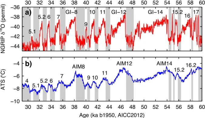
Figure S4 a) Water-stable-isotope record (δ18O) from the North Greenland Ice Core Project (NGRIP) with Greenland Interstadial (GI) labels and timing according to Rasmussen et al. [2014]. b) Antarctic Temperature Stack (ATS) based on stacked water-stable-isotope records (δ18O and δD) from six Antarctic ice cores: EPICA Dome C, EPICA Dronning Maud Land (EDML), Vostok, Talos Dome, and Dome Fuji as published in Parrenin et al. [2013], to which we have added borehole-calibrated δ18O-based temperatures from the WAIS Divide core [WAIS Divide Project Members, 2015].
Temperature is expressed as an anomaly with respect to the past millennium. The Antarctic Isotope Maxima (AIMs) are labeled following the nomenclature in EPICA Community Members [2006]. Note how warming phases of AIMs coincide with Greenland Stadials (grey shading) and cooling phase of AIMs coincide with Greenland Interstadials. The records span Marine Isotope Stage 3 with the time axis is in thousand of years before 1950 AD, on the Antarctic Ice Core Chronology 2012 (AICC2012; Veres et al., [2013]). Note that the Greenland temperature variations of ~5–16°C [Kindler et al., 2014] are much larger than the Antarctic temperature variations.
6 Table S1. Summary of the annual mean heat-flux anomalies in the 50–70°S zonal band during the stage 1 active Southern Ocean (SO) deep convection (blue shading in Figure 2) and during the stage 2 maximum in Antarctic warming (red shading in Figure 2).
Anomalies are calculated with respect to the long-term mean. Positive values signify a gain of energy for the 50–70°S atmospheric column. See also the Figure 4 schematic.
Abbreviations: surface heat-flux anomaly (SHF); meridional heat-transport anomaly (MHT); top of atmosphere heat-flux anomaly (TOA).
Stage 1
Active SO deep convection
Stage 2
Maximum Antarctic warming
Process Strength
(Wm-2)
Strength (TW)
Strength (Wm-2)
Strength (TW)
SHF +0.19 +9.7 -0.22 -11.1
Sea-ice–albedo feedback +0.76 +38.0 +0.52 +26.1
Cloud feedback -0.66 -32.7 -0.42 -21.0
(TOA) (0.1) (5.3) (0.1) (5.1)
Atmospheric MHT across 50°S -0.26 -12.8 +0.24 +11.9
Atmospheric MHT across 70°S -0.04 -2.1 -0.12 -5.9
Sum 0.0 0.1 0.0 0.0
References
EPICA Community Members (2006), One-to-one coupling of glacial climate variability in Greenland and Antarctica, Nature, 444, 195–198, doi:10.1038/nature05301.
Kindler, P., M. Guillevic, M. Baumgartner, J. Schwander, A. Landais, and M.
Leuenberger (2014), Temperature reconstruction from 10 to 120 kyr b2k from the NGRIP ice core, Clim. Past, 10, 887–902, doi:10.5194/cp-10-887-2014.
Parrenin F., et al. (2013), Synchronous change of atmospheric CO2 and Antarctic temperature during the last deglacial warming, Science, 339(6123), 1060–1063, doi:
10.1126/science.1226368.
Rasmussen, S. O. et al. (2014), A stratigraphic framework for abrupt climatic changes during the last glacial period based on three synchronized Greenland ice-core records:
refining and extending the INTIMATE event stratigraphy, Quat. Sci. Rev., 106, 14–28, doi: 10.1016/j.quascirev.2014.09.007.
Veres, D. et al. (2013), The Antarctic ice core chronology (AICC2012): An optimized multi-parameter and multi-site dating approach for the last 120 thousand years, Clim.
Past, 9, 1733–1748, doi:10.5194/cp-9-1733-2013.
WAIS Divide Project Members (2015), Precise interpolar phasing of abrupt climate change during the last ice age, Nature, 520, 661–665, doi:10.1038/nature14401.