CLIVAR Exchanges

CLIVAR Exchanges

CLIVAR Open Science Conference Award Winners

Participants of the CLIVAR Early Career Scientists Symposium, FIO/SOA, Qingdao, China

Editorial

Nico Caltabiano

International CLIVAR Project Office, Southampton, UK

The past year was an amazing year for CLIVAR. The celebration of our 20 years of success culminated with the CLIVAR Open Science Conference in September.

Almost 700 scientists from 50 countries gathered in Qingdao, China, and over the course of five days, scientists showcased major advances in climate and ocean research.

By design, more than one third of participants were early career scientists, who presented their work through 234 posters and oral presentations, including plenary talks.

One of the important aims of the conference was to engage the future generation. Jointly with the OSC, CLIVAR successfully organized an Early Career Scientists Symposium (ECSS), hosted by China’s First Institute of Oceanography (SOA/FIO). More than 120 students and early career scientists participated in the symposium.

Participants enjoyed an informal atmosphere, while discussing in groups the key research challenges that the scientific climate community faces at the moment and highlighting the need for international science collaboration. They also discussed the best ways to engage potential stakeholders with their scientific information and suggested their vision for the future of CLIVAR. I would like to say a big thank you to all those involved in the organisation of the ECSS. Without them, the success of the symposium would not have been possible.

The conference injected an amazing degree of enthusiasm about CLIVAR’s research and fortified the notion that CLIVAR is and will be critical to meet society’s needs for climate information. International cooperation of the type that CLIVAR fosters will continue to be indispensable to developing the human capacity and infrastructure that underpin all major scientific breakthroughs.

The conference certainly helped in handing over the enthusiasm for CLIVAR and its science to the next generation, whose excitement is a promise for a very bright future. This issue of Exchanges showcases some of high quality research done by young researchers that were presented with outstanding poster awards at the OSC. A team of over 50 senior and early career scientists reviewed the 234 qualifying posters, and the full list of winners can be seen at this url: http://www.clivar.org/

news/clivar-osc-poster-awards.

Also, this past year saw the departure of Valery Detemmerman from the ICPO. Valery has supported CLIVAR activities for more than two decades, initially from her position at the WCRP’s Joint Planning Staff (JPS)

in Geneva, and then as the Executive Director of the ICPO in Qingdao, since 2014. Valery is now enjoying a well deserved retirement, and her always optimistic approach will be missed by all in the CLIVAR community.

But we are also pleased that, after an extensive search, we would like to welcome the new Executive Director of the International CLIVAR Project Office (ICPO), José Luis Santos Davila. José obtained his Ph.D. in Atmospheric Sciences from the Georgia Institute of Technology of Atlanta, USA in 1995. He has been a Professor at the Marine Sciences and Maritime Engineering Department of the Escuela Superior Politecnica del Litoral, located in Guayaquil, Ecuador since 1989. He was the Director of the International Research Center on El Niño (CIIFEN) between 2002-2005. His current research interest are El Niño-Southern Oscillation variability and impacts, and Climate Change and variability on tropical areas. The ICPO Executive Director will be based at the International CLIVAR Global Project Office, generously hosted at the First Institute of Oceanography (FIO), in Qingdao, China.

José will move to Qingdao and officially start on his position at the beginning of April.

Noel C. Baker, Eric Behrens, Julius Busecke, Victor Dike, Jonathan V.

Durgadoo, Ariane Frassoni, Sarah Kang, Gaby Langendijk, Debashis Nath, Kevin Reed, Neil Swart

The CLIVAR Early Career Scientists Symposium was hosted by the First Institute of Oceanography in Qingdao, China, on September 18 and 24-25, 2016. 135 early career scientists (ECS) from 34 countries participated.

The first day of the symposium provided the opportunity for ECS to network with peers and senior scientists, to become familiar with the institutional structure of CLIVAR, and to prepare for the upcoming Open Science Conference (OSC). During the weekend following the OSC, the symposium served as a forum to actively engage the ECS and challenge them to find solutions to critical issues in atmospheric and ocean science. Participants worked in diverse international teams to complete the following tasks: highlight key research challenges and goals; identify major challenges facing international science collaboration; discuss how to effectively engage the audience of their scientific information; and suggest their vision for the future of CLIVAR.

As the next generation of scientists, the ECS participants recognized their critical role in shaping the future of climate science by answering pressing research challenges and goals. In agreement with CLIVAR’s Science Challenges outlined in the Science Plan, ECS participants emphasized the need for improved understanding of 1) regional climate change and variability, 2) internal variability, 3) ocean carbon and heat uptakes, and 4) climate processes and feedbacks. The community would also benefit from coordinated climate model developments, an improved and expanded global observation network, and further efforts towards seamless prediction across space and time scales. The ECS recognized the need for increased interdisciplinary research and are committed to bridging the gaps between disciplines.

International collaboration was highlighted as instrumental to the success of the global science community, as the ECS recognized that climate challenges are not contained by political borders, and international cooperation is critical for developing solutions. Collaboration is dampered by asymmetries between nations, which include: unequal access to data and journals, unequal funding and resources, language barriers, and political limitations such as overly-restrictive visa requirements which too often hinder travel. Potential

solutions include two-way collaborative exchanges of scientists between countries, promoting regional networks and capacity building (particularly within developing nations), and encouraging participation in international networks and organizations to link scientists and increase visibility of their work. An overarching theme which emerged repeatedly at the symposium was the need for increased openness and standardization of scientific content such as access to journal articles, open- source code, and universal accessibility and increased standardization of data. A proposed solution to address travel restrictions due to cumbersome visa requirements is for CLIVAR to take a leading role as a global entity representing climate scientists to formulate an open letter highlighting the issue and addressing it to local science ministries and foreign affairs departments.

Education at all levels, from schools to seniors, was seen as key to engaging the audience of information produced by the climate science community. An active debate emerged on the appropriate spread of CLIVAR efforts between conducting core scientific research versus engaging in communication. It was recognized that effectively informing adaptation measures would require far greater inclusion of “external disciplines,”

including the social sciences, engineering and planning communities, while still requiring significant input from the CLIVAR science community.

The ECS expressed general support for the priorities and implementation strategies laid out in the CLIVAR Science Plan while making concrete suggestions for improving the plan to better reflect the full community.

The next generation of climate scientists is dedicated to overcoming the challenges outlined in this summary and looking forward to advancing CLIVAR’s mission and activities by leveraging the new ideas and collaborations forged at the 2016 ECS Symposium.

A further article titled "Summary of the CLIVAR Early Career Scientists Symposium 2016”, with an overview of the activities of the ECC Symposium, has been submitted to Nature Climate and Atmospheric Science, and should be published soon.

Reflections on the CLIVAR Early Career

Scientists Symposium 2016

Rondrotiana Barimalala

, Annalisa Bracco

, Lei Zhou

1Shanghai Jiao Tong University, Shanghai, China

2Georgia Institute of Technology, Atlanta, GA, USA Contact e-mail: rbarimal@sjtu.edu.cn

Introduction

Studies on interannual variability in biogeochemistry are still limited in the tropical Indian Ocean (IO), particularly with regard to the air-sea CO₂ gas exchanges. Existing studies, mostly focused on annual means and seasonal variability, present large uncertainties as observations spread in space and time over IO are still lacking. For instance, using ship observational data, Takahashi et al. (2009) found that the tropical Indian Ocean is a source of CO₂ to the atmosphere with an annual mean of 0.09±0.005PgC.yr^-1. Similarly Valsala et al. (2013) found that the Indian Ocean is a source of 0.12±0.04PgC.yr^-1 to the atmosphere using a simple ocean biogeochemical model. On the other hand, Gurney et al. (2004) found that the Indian Ocean is a sink of CO₂ with an annual mean of 0.32±0.33PgC.yr^-1 using inverse techniques.

Previous studies show that changes in physical climate can affect the exchange of CO₂ between the atmosphere, land and ocean. The resulting changes in CO₂ concentration in turn affect the physical climate, through the so-called climate-carbon feedback (e.g.

Friedlingstein et al., 2006, Arora et al., 2013). The well- known interannual variability in the IO might, therefore, affect the air-sea CO₂ variability, that can then feedback to its physical modes. However, most studies on air-sea CO₂ fluxes and their interannual variability are focused on the tropical Pacific and Atlantic as the Indian Ocean does not contribute significantly to the global CO₂ flux variability (e.g, Le-Quere et al., 2000; McKinley et al., 2004; Valsala et al., 2014; Wang et al., 2015). Nevertheless, although the IO air-sea CO₂ variability may not contribute on a global scale, it can play an important role regionally.

Among the few existing studies, Valsala et al. (2013) found that the interannual anomalies of CO₂ emission over the northern Indian Ocean are about 30% to 40%

of the seasonal amplitudes. However, due to the biases and magnitude errors in their analyses, which may be due to lack of an ecosystem module in their model, they suggest that further studies are needed. Recently,

the fifth Coupled Model Intercomparison Project (CMIP5 - Taylor et al., 2012) provides a large enough ensemble of Earth System Models (ESM) designed to simulate the interaction between physical, chemical and biological processes in the atmosphere, land and ocean to allow for reconsidering this problem.

The aim of this study is therefore to evaluate how the CMIP5-ESM models represent the interannual variability of surface pCO₂ partial pressure and air-sea CO₂ flux over the Indian Ocean. Moreover, we seek to investigate the linkages between pCO₂ variability and the well-known physical modes that impact the Indian Ocean circulation:

the El-Niño Southern Oscillation (ENSO) and the Indian Ocean Dipole (IOD). Four models from the CMIP5-ESM are analyzed in this work. Overall, the models depict a realistic seasonal cycle in surface pressure CO₂ (spco₂) and air-sea CO₂ fluxes (fgco₂). The whole IO (north of 30^oS) is found to be a net sink in CO₂ both in the observations (with an annual mean of 0.06PgC.yr^-1) and in the models (with an annual mean ranging from 0.003PgC.yr^-1 to 0.05PgC.yr^-1). In the models, the interannual variability in fgco₂ varies from 25% to 95% of the respective seasonal amplitude. However, further investigation is needed to explain the driving mechanisms of the air-sea CO₂ flux interannual variability as no precise conclusion could be deduced from the present study.

Models and data description

Outputs from four models participating in the CMIP5- ESM ensemble are analyzed in this study. These models are used based on the availability of the data when the analysis was initiated. However a more complete set of the models will be published in a later report.

The models are CESM1-BGC, GFDL-ESM2G, HadGEM2- ES and MPI-ESM-LR. One realization from each model is used. Monthly mean from the outputs are utilized through the study. We focus on the historical simulations

Indian Ocean sea surface partial pressure CO

and air-sea CO

flux interannual variability in

the CMIP5-ESM models

and on the period extending from 1950 to 2005.

We also use the HadISST reanalysis (Rayner et al., 2003) as observational counterpart of sea surface temperature (SST), and the climatological data from Takahashi et al. (2009) to evaluate the spco₂ and fgco₂ fluxes. The anomalies of any given variable throughout this study are calculated as the difference between the variable and the time dependent mean for the period of study.

Nino3.4 index defined as the area average of SST anomalies within 190E-210E, 5S-5N is used to represent ENSO, and the IOD index is defined as the difference between the area average SST anomalies within east IO (EIO; 90E - 110E, 10S - 0) and west IO (WIO; 50E-70E, 10S - 10N).

Climatology

Fig 1 shows the climatological SST, spco² and fgco₂ (downward positive) averaged over the whole IO domain (30E-110E, 35S-30N). In general, the models represent well the seasonal cycle of these three variables.

For SST, the highest mean temperature occurs during boreal spring, in correspondence with the monsoon reversal period. The lowest temperature is seen in late boreal summer when different upwelling systems over the basin (e.g., Somalia upwelling system, east IO) are at their peak.

Compared to the observations, CESM1-BGC shows a warm bias throughout the year, whereas the other three models are colder than HadISST, with HadGEM2-ES being the closest to the observations, except for April.

Similarly, the spco₂ annual cycle has its maximum in boreal spring and minimum in August, confirming the partial role of SST in driving the spco₂. The annual variation in spco² throughout the year is around 2Pa.

HadGEM2-ES shows the strongest bias with respect to the climatological observations of Takahashi et al.

(2009), while the other three models are close to each other and displaying weaker levels than the observations, especially from June onward.

On the other hand, the air-sea CO₂ flux reaches a maximum during boreal summer season and a minimum in winter. In this study, positive fgco₂ represents flux from the atmosphere into the ocean. In the observational reanalysis the whole IO is therefore a net sink of CO₂(0.06PgC.yr^-1) in all months. The models, however, display negative fgco₂ (source to the atmosphere) in winter extending into spring and early boreal summer depending on the model. On average, the annual mean in fgco₂ is found to be 0.047PgC.yr^-1 in CESM1-BGC, 0.05PgC.

yr^-1 in GFDL-ESM2G, 0.01PgC.yr^-1 in HadGEM2-ES and 0.003PgC.yr^-1 in MPI-ESM-LR. By separating the north and south IO, the models agree with previous studies,

Figure 1: Seasonal cycle averaged over the India Ocean (30E-110E, 35S-30N) for (a) SST (Units: degree C), (b) ocean surface pco₂ (Units: Pa) and (c) air-sea CO₂ flux in which positive sign represents a downward flux (Units: PgC.yr^-1)

Figure 2: SST first EOF for (a) HadISST, (b) CESM1-BGC, (c) GFDL-ESM2G, (d) HadGEM2-ES, (e) MPI-ESM-LR. (Units:

degree C)

suggesting that the north IO is a perennial source of CO₂ to the atmosphere, whereas the south is a sink (e.g. Sarma et al., 2013). The magnitudes of CO₂ fluxes are mostly underestimated in the models, except during boreal summer when GFDL-ESM2G depicts higher fgco² than in the observational data set.

Long-term trend and interannual variability

Before analyzing the interannual variability in spco₂ and fgco₂, the model representation of the dominant climate modes in SST is evaluated with an Empirical Orthogonal Function (EOF) analysis. This is important given that the surface ocean temperatures are a major driver of thespco₂ (and therefore fgco₂) seasonal cycle and they are likely to influence the interannual variability as well.

All interannual analyses are computed after removing the linear trend in the data and using a 12 months running mean of the monthly data from 1950-2005.

Figure 3: (a) spco₂ interannual variability (continuous line) and linear trend (dashed line). spco₂ first EOFs for CESM1- BGC (b) CESM1-BGC, (c) GFDL-ESM2G, (d) HadGEM2-ES, (e) MPI-ESM-LR(Units: Pa)

Fig 2 shows the first EOF (EOF1) of the SST anomalies in the HadISST reanalysis and in the models. The observational data set displays a basin-wide warming, in which the first Principal Component (PC1) is significantly correlated to the Nino3.4 time series (corr = 0.57) and explains 31% of the total variance, whereas PC2 (not shown) is significantly linked to the IOD index (corr 0.32) In general, the models reproduce the observed dominant modes. For instance, CESM1-BGC, GFDL- ESM2G and MPI-ESM-LR depict the basin wide warming as EOF1, explaining respectively 36%, 33.6% and 29.9%

of their total variances. The correlations between PC1 and Nino3.4 in these three models are higher than in the observations (0.62, 0.63 and 0.65, respectively).

In HadGEM2-ES the EOF1 pattern mostly consists of a positive anomaly but a cooling signal can be seen in the eastern part of the basin, forming a dipole-like pattern.

The correlation between PC1 and Nino3.4 is also lower (0.63) than that of PC1-IOD (0.68), suggesting that the dominant mode of variability in this model is the IOD.

The temporal evolution of the IO spco₂ anomalies in the CMIP5-ESM models are shown in Fig 3a. Continuous lines show the linearly detrended anomalies, and dashed lines represent the linear trends for each model. Overall the models show positive trends up to 1.8Pa.decade^-1. By considering the whole period of 1950-2005, a change in linear trend is noticed in the models. Change in trend detection technique is therefore applied and the models depict an acceleration of trend from after 1975 compared to previous years. These two linear trends are then removed from the models accordingly. However, no observational data can be used to verify such change in the trend.

The interannual anomalies in spco₂ have relatively weak magnitude with respect to the trend, and are contained within ±0.3Pa. The patterns of the first EOFs in spco₂ (Figs 3b-e) show quite a disagreement between the models. For instance, CESM-BGC displays a dipole-like pattern with an increase in spco₂ in the east IO and a decrease in the west. EOF1 explains 55% of the total variance. The correlation between PC1 with Nino3.4 and IOD are respectively 0.4 and 0.63. The relatively high correlation between PC1 and IOD suggests that the dominant mode of variability in spco₂ for CESM1-BGC is the IOD. For GFDL-ESM2G and HadGEM2-ES, the EOF1 is characterized by a basin-wide increase in spco₂, which explains about 23% of the variance. The correlations between PC1 and Nino3.4 are respectively 0.43 and 0.56 in the two models. The correlation between PC1 and IOD, however, is not statistically significant for GFDL-ESM2G and is 0.36 for HadGEM2-ES. Thus, for these two models, ENSO modulates the spco₂ interannual variability. Finally in MPI-ESM-LR, although EOF1 represents 21% of the total variance, the dominant mode does not show any significant correlation with either of the two physical modes.

Fig 4a shows the area integrated interannual anomalies of fgco₂ in the IO. For the period of 1950-2005, all models show a weak upward fgco₂ trend in which CESM1-BGC displays the highest trend of 0.008PgC.

decade^-1 and GFDL-ESM2G shows the lowest at 0.002PgC.

decade^-1.The amplitudes of the interannual anomalies range between -0.025PgC.yr^-1 and 0.03PgC.yr^-1, about 25% to 95% of their respective seasonal amplitudes.

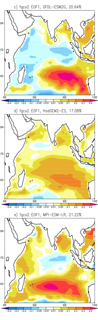
The first EOFs of fgco₂ in the IO explain respectively 41.9%, 20.6%, 17.1% and 21.2% of the variance for CESM1-BGC, GFDL-ESM2G, HadGEM2-ES and MPI-ESM- LR. In the four models, common patterns of positive air- sea CO₂ flux are seen over the south IO (mainly along the thermocline ridge) and the Bay of Bengal. These are known areas of net sink CO₂ in the IO. In other parts of the basin, the models show a significant mismatch. For instance, the eastern equatorial IO is a CO₂ sink in CESM1- BGC and HadGEM2-ES, but it is a source in the other two models. Moreover, in the western IO, CESM1-BGC and GFDL-ESM2G depict negative fgco₂ whereas HadGEM-ES and MPI-ESM-LR show positive anomalies.

Overall, the EOF pattern for CESM1-BGC clearly reflects the influence of the IOD on the air sea CO₂ flux; the correlation between PC1 and IOD is 0.62. For GFDL- ESM2G, and HadGEM-ES, although the dominant mode in spco₂ is linked to ENSO, the correlation between fgco₂ PC1 and Nino3.4 (0.27 for GFDL-ESM2G and 0.48 for HadGEM-ES) does not differ much from that of PC1 and IOD (0.28 and 0.51). Similar correlations are also found in MPI-ESM-LR, despite the fact that the correlation between the two physical modes with spco₂ was not statistically significant.

No clear conclusion on the relative role of IOD and ENSO can be deduced yet from these last three models. These results need further investigation given that the effect of ENSO and IOD in these models could be complementary throughout the fifty year-period of study (as found by Valsala et al. (2013) in their work on the Northern IO), triggering very close correlations between PC1 and each of the indices.

Summary

Outputs from 4 models within CMIP5-ESM are used to investigate the interannual variability in spco₂ and air- sea CO₂ flux in the tropical Indian Ocean. The models reproduce reasonably well the seasonal cycle over the whole IO. However, the interannual variability along with the dominant driving mechanisms differs considerably between the models. The IOD is found to be the main driver of the air-sea CO₂ flux variability in CESM1-BGC, while both the IOD and ENSO appear to play a comparable role in the other models. A closer look at different parts of the IO will also help understanding the CO₂ interannual variability and its mechanisms over the

Figure 4: Same as Fig 3 but for fgco₂ (Units: 10-1PgC.yr^-1) basin. In addition, to better quantify the contribution of the physical forcings, a decomposition of the spco₂ responseto SST, salinity, alkalinity and dissolved inorganic carbon changes should be performed.

References

Arora, V., G. Boer, P. Friedlingstein, et al. 2013: Carbon- concentration and carbon-climate feedbacks in CMIP5 Earth system models. J. Climate. doi:10.1175/

JCLI-D-12-00494.1

Friedlingstein P., P. Cox, R. Betts et al. 2006: Climate-carbon cycle feedback analysis: results from the (CMIP)-M-4 model intercomparison. J. Climate, 19, 3337–3353.

Gurney K.R., R.M. Law, A.S. Denning, P.J. Rayner, B. Pak 2004: Transom-3-L2-modelers Transcom-3 inversion intercomparison: model mean results for the estimation of seasonal carbon sources and sinks. Glob Biogeochem Cycles 18. doi:10.1029/2003GB002111

Le-Quere C., J.C. Orr, P. Monfray, O. Aumont, G. Madec 2000:

Interannual variability of the oceanic sink of CO2 from 1979 through 1997. Glob Biogeochem Cycles 14:1247–

1265

McKinley G.A., M.J. Follows, J. Marshall 2004: Mechanism of air-sea CO2 flux variability in the equatorial Pacific and North Atlantic. Glob Biogeochem Cycles 18.

Doi:10.1029/2003GB002179

Rayner N.A., D.E.Parker, E.B. Horton et al. 2003: Global analysis of SST, sea ice and night marine air temperature since the late nineteenth century. J Geophys Res.

Doi:10.1029/2002JD002670.

Sarma V. V. S. S., A. Lenton , R.M. Law et al. 2013: Sea-air CO2 fluxes in the Indian Ocean between 1990 and 2009.

Biogeosciences, 10, 7035-7052. doi:10.5194/bg-10-7035- 2013.

Takahashi T., S.C. Sutherland, R. Wanninkhof, C. Sweeney, R.A. Feely 2009: Climatological mean and decadal changes in surface ocean pCO2, and net sea–air CO2 flux over the global oceans. Deep-Sea Res Part 2, 56,554–577.

Taylor K.E., R.J. Stouffer, G.A. Meehl 2012: An overview of CMIP5 and the experiment design. Bulletin of the American Meteorological Society, 93, 4: 485-498.

Valsala V.,S. Maksyutov 2013: Interannual variability of the air-sea CO2 flux in north Indian Ocean. Ocean Dynamics 63, 165. Doi:10.1007/s10236-012-0588-7

Valsala V., M.K. Roxy, K. Ashok, R. Murtugudde 2014:

Spatiotemporal characteristics of seasonal to multidecadal variability of pCO2 and air-sea CO2 fluxes in the equatorial Pacific Ocean. Journal of Geophysical Research: Oceans, 119, 12, 8987-9012. doi: 10.1002/2014JC010212

Wang X., R. Murtugudde, E. Hackert, J. Wang, J. Beauchamp 2015: Seasonal to decadal variations of sea surface pco2 and

sea-air CO2 flux in the equatorial oceans over 1984-2013: A basin-scale comparison of the Pacific and Atlantic Oceans.

Glob Biogeochem Cycles 29. Doi:10.1002/2014GB005031.

Nils Brüggemann

, Caroline A. Katsman

, Henk A. Dijkstra

1Delft University of Technology, Netherlands

2Institute for Marine and Atmospheric Research Utrecht, Netherlands Contact e-mail: n.bruggemann@tudelft.nl

Introduction

The zonally averaged transport in the Atlantic, the Atlantic Meridional Overturning Circulation (AMOC), is responsible for a maximum northward heat transport of about 1PW (Trenberth and Caron, 2001). It is therefore a key player in the climate system and subject of many climate research studies. Despite the enormous research effort, open questions regarding e.g. the strength and sensitivity of the AMOC remain. Especially, it is unclear how the AMOC changes in the course of projected climate change. This article is intended to give a brief introduction about our approach to better understand where and how the northward flowing water masses sink before they return southward at depth. In particular, we aim to investigate which dynamical processes are involved in this sinking process that we refer to as the downwelling branch of the AMOC.

Idealized studies indicate that the downwelling is confined to lateral boundary currents around the marginal seas of the North Atlantic (e.g. Spall, 2001; Straneo, 2006; Spall, 2010). These studies further indicate that eddies play an important role for the downwelling since they influence e.g. the heat and vorticity budget of the boundary current.

This than effects the horizontal convergence of the flow and therefore the downwelling itself.

In the presence of rotation, vertical motion is linked to a change of vorticity. Spall (2010) and Cenedese (2012), use the vorticity budget to identify how the downwelling causing a vorticity stretching is balanced by other terms in the vorticity balance. They find that vorticity advection and dissipation plays an important role in balancing the stretching.

We follow the approach of Spall (2010) and Cenedese (2012) and diagnose the vorticity budget but further expand it by separating the mean advection term from the eddy advection term. This enables us to distinguish between the role of the mean flow and that of the eddies on the downwelling. Beside using idealized studies similar to that of Spall (2010), we also diagnose the vorticity budget in a more realistic strongly-eddying (0.1 degree) global ocean model.

The downwelling in a realistic configuration

The realistic model that we use to diagnose the downwelling and the vorticity budget is a strongly- eddying configuration of POP (Parallel Ocean Program) with a nominal grid spacing of 0.1°and 42 vertical levels (Maltrud et al., 2010). The model is forced by the “normal year” Coordinated Ocean Reference Experiment (CORE) forcing dataset. This dataset, consists of a single annual cycle that is repeated every model year (Large and Yeager, 2004). Details of the model configuration can be found in the auxiliary material of Weijer et al. (2012).

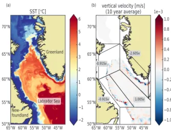
Fig 1a shows the sea surface temperature in the Labrador Sea in winter. It shows a warm boundary current circulating anti-clockwise around the colder interior of the Labrador Sea. At the west coast of Greenland a topographic narrowing destabilizes the boundary current and warm-core anti-cyclonic eddies form. These eddies play an important role in exchanging heat and vorticity between the boundary current and the interior.

All along the boundary current, patterns of enhanced vertical velocities can be found (Fig. 1b) often with alternating signs. Since Fig. 1b was derived from a 10 year mean, the alternating up- and downwelling signal cannot be associated with mesoscale eddies.

An exception to this alternating up- and downwelling signal can be found downstream of Cape Desolation in the West Greenland Current. Here, a large stripe of downward velocities can be identified, accompanied by a weaker upwelling signal further offshore. This strong downwelling signal is responsible for most of the net downwelling in the Labrador Sea and therefore of particular interest for this study.

The downwelling in an idealized configuration

To further investigate the dynamics that are involved in the downwelling, we use an idealized model configuration.

The main aim of this idealized model simulation is to reproduce the basic circulation of the Labrador Sea, in particular the enhanced downwelling pattern offshore of Cape Desolation. At the same time, we try to avoid

On the vorticity dynamics of the downwelling

branch of the AMOC

generating complicated patterns of up- and downwelling as found in the realistic model (Fig. 1b) by using a simplified topography.

Our idealized model configuration of the MITgcm is similar to that one used by Spall (2010). The model domain consists of a closed basin with a simple topography that decays exponentially from the lateral boundaries towards the interior (see Fig. 2). By increasing the e-folding scale of the topographic slope, we introduce a topographic narrowing at the eastern part of our domain. This topographic narrowing is mimicking the steep slopes offshore of Cape Desolation.

We use a horizontal resolution of 2km and 20 vertical levels of 150m, yielding a maximum depth of 3000m.

By using partial bottom cells, we obtain a smoother representation of the topographic slope. Further idealizations of our model consist of applying the beta- plane approximation and using a linear equation of state with temperature as the only active tracer. Biharmonic dissipation and diffusion operators are applied with no-slip boundary conditions at the lateral and bottom boundaries.

A warm boundary current, representing current systems like the West Greenland Current, is induced by restoring temperature in the southernmost part of the domain to a reference profile with constant vertical and meridional gradients. Furthermore, we restore velocity in this region to be in thermal wind balance and add a barotropic component such that there is a zero flow at the bottom.

We represent surface cooling by applying a constant heat flux of 50 W/m². In cases of static instability, we increase the vertical diffusivity as a parameterization of convection since our simulations are hydrostatic.

After a spin-up of five years, the flow field is in statistical equilibrium. A warm boundary current is established (Fig. 2a) and a rich warm-core anti-cyclonic eddy field is responsible for exchanging heat between the warm boundary current and the cold interior balancing the surface heat loss (Fig. 2a and b). The mean flow derived from a five-year average following a five year spin-up demonstrates enhanced vertical velocities along the topographic narrowing, with a downward transport of 4.4Sv (Fig. 2c).

The vorticity budget

Spall (2010) used the vorticity budget in a similar setup as our idealized configuration to find that stretching of planetary vorticity is primarily balanced by eddy flux divergences of relative vorticity and, close to the lateral boundary, by friction. We expand the diagnostics of Spall (2010) by separating the vorticity advection term into a mean and an eddy component. This facilitates the explanation of both terms but most importantly, it allows to separate the role of the eddies from that of the mean flow.

In fact, we find that both terms are of similar magnitude but play a different role in setting the downwelling. The mean flow is most dominant up- and downstream of the narrowing where the topographic slope changes and the current converges. It has a strong downward component upstream and slightly weaker upward component downstream of the narrowing. It therefore indicates how a topographic sill can induce strong down- and upward motion. We speculate that similar topographic features are responsible for the complicated up- and downwelling patterns in the realistic model (Fig. 1b).

The eddy term is most dominant at the narrow slope Figure 1: Circulation of the realistic strongly eddying ocean

simulation. (a) Wintertime sea surface temperature (SST) snapshot of model year 302 and (b) vertical velocity at 1000m averaged over 10 years (year 296 to 306) Labelled values in (b) denote vertical transports over marked regions.

Figure 2: Snapshot of (a) sea surface temperature and (b) surface vertical vorticity component after 9.5 years; (c) five year average (year 6 to 10) of vertical velocity at 900m. Grey lines denote topography contours with intervals of 500m.

Averaging the vertical velocity over the region indicated by the black square yields a net downwelling of 4.4Sv.

itself. As found by Spall (2010), the eddy component of the vorticity advection is towards the boundary. Therefore, it induces vorticity stretching offshore and vorticity squeezing onshore. Indeed, the offshore stretching can be identified with the strong downwelling pattern along the topographic narrowing (Fig. 2c). However, there is no upwelling signal onshore. Here, dissipation and the mean component of the vorticity advection cancel the eddy component of the vorticity advection.

Conclusion

The aim of this study is to better understand the dynamics of enhanced downwelling and therewith to better understand the downwelling branch of the AMOC.

Measuring vertical velocities remains a challenge and observations of vertical velocities barely exist. Therefore, we use a combination of realistic and idealized models to study the downwelling. With the idealized simulations, we are able to focus on the most crucial dynamical processes contributing to the downwelling. By excluding e.g. complex topographic features, the downwelling pattern becomes more regular and easier to interpret.

Diagnosing the dynamics that are involved in the downwelling of the idealized model then facilitates to interpret the more complex downwelling patterns in the realistic model simulation.

Finally, we think that our results are helpful for understanding and interpreting the sensitivity of the dynamics involved in the downwelling branch of the AMOC. In particular, we expect to gain more insight into the sensitivity of the downwelling or the eddy activity with respect to external parameters like the wind stress or surface heat fluxes over marginal seas like the Labrador Sea.

Acknowledgments

We would like to thank Michael Kliphuis in supporting us with the POP simulations. The simulations have been performed on the Cartesius supercomputer at SURFsara (https://www.surfsara.nl) through the projects SH-350- 15 and SH-284. Funding for Nils Brüggemann is provided by the Netherlands Organisation for Scientific Research (NWO-ALW VIDI grant 864.13.011 awarded to Caroline Katsman).

References

Cenedese, C., 2012: Downwelling in Basins Subject to Buoyancy Loss. J. Phys. Oceanogr., 42, 1817-1833

Large W. G. & Yeager, S., 2004: Diurnal to decadal global forcing for ocean and sea-ice models: The data sets and flux climatologies. NCAR Technical Note NCAR/TN- 460+STR

Spall, M. A., 2010: Dynamics of Downwelling in an Eddy- Resolving Convective Basin. J. Phys. Oceanogr., 40, 2341- 2347

Straneo, F., 2006: On the Connection between Dense Water Formation, Overturning, and Poleward Heat Transport in a Convective Basin. J. Phys. Oceanogr., 36, 1822-1840

Trenberth, K. E. & Caron, J. M., 2001: Estimates of Meridional Atmosphere and Ocean Heat Transports. J.

Climate, 14, 3433-3443

Weijer, W.; Maltrud, M. E.; Hecht, M. W.; Dijkstra, H. A.

& Kliphuis, M. A., 2012: Response of the Atlantic Ocean circulation to Greenland Ice Sheet melting in a strongly- eddying ocean model. Geophys. Res. Lett., 39

Leandro B. Díaz, Carolina S. Vera, Ramiro I. Saurral

Centro de Investigaciones del Mar y la Atmósfera/CONICET-UBA DCAO/FCEN, UMI-IFAECI/CNRS, Buenos Aires, Argentina

Contact e-mail: ldiaz@cima.fcen.uba.ar

Introduction

The climate changes observed in the last decades have raised concern among policy and decision makers about the importance of improving the knowledge and prediction of climate. In particular, the Southeastern South America (SESA) is one of the few regions in the world which have experimented both large positive summer precipitation trends in mean and extremes during the 20th century (e.g. Liebmann et al., 2004; Re and Barros, 2009; Penalba and Robledo, 2010; Saurral et al., 2016). Furthermore, a precipitation increase is projected over the region for the current century (Hartmann et al., 2013). These changes pose a significant threat for many socio-economic sectors within this region.

Recently, Vera and Díaz (2015) have shown that the fifth phase of the Coupled Model Intercomparison Project of the World Climate Research Program (CMIP5, Taylor et al., 2012) multi-model historical simulation dataset (i.e.

including all observed forcings) is able to represent the sign of the trends of the last century over SESA, although with a weaker magnitude. When comparing results from the historical simulation including all forcings against those only including natural forcings and only considering greenhouse gases forcing, they concluded that anthropogenic forcing in CMIP5 models has a detectable influence in explaining the observed positive precipitation trends.

Through teleconnection patterns, tropical ocean variability is one of the main precipitation forcings in SESA. The El Niño Southern Oscillation (ENSO) has been shown to be the main influence for SESA rainfall variability on interannual scales (e.g. Ropelewski and Halpert, 1987; Kiladis and Diaz, 1989). However, the way in which ENSO affects SESA rainfall seems to be modulated by ocean lower-frequency patterns as the Pacific Decadal Oscillation (PDO) (Kayano and Andreoli, 2007) and the Atlantic Multidecadal Oscillation (AMO) (Kayano and Capistrano, 2014). Furthermore, Barreiro et al. (2014) found that both, PDO and AMO, have also an influence on summer SESA rainfall independently from ENSO.

How anthropogenic forcings are combined with low frequency natural climate variability to modulate the regional rainfall variability and trends in SESA has not been explored in detail yet. Therefore, a deeper knowledge of decadal climate variability in the region is needed in order to project near term future changes with a larger degree of confidence. According to this, our goal is to understand the influence of the large-scale interannual variability of sea surface temperatures (SST) on austral summer rainfall in SESA in a global warming context and to evaluate if CMIP5 models are able to represent that influence properly.

Leading observed co-variability pattern of SST and SESA rainfall

Rainfall data from the Global Precipitation Climatology Centre (GPCC) dataset (Schneider et al., 2011) were used in this study, with a spatial resolution of 2.5°. This product considers station-based records, and thus it only has continental coverage. SST monthly values were derived from the NOAA Extended Reconstructed Sea Surface Temperature Version 3b (ERSSTv3b, Smith et al., 2008) with a spatial resolution of 2°. Summer was defined as the December–January–February (DJF) trimester.

Anomalies were computed from the corresponding long- term means considering the period 1902–2010. Both undetrended and detrended anomalies were defined for both variables. Non-linear trends were removed through a linear regression between global mean SST time series and those for SST or precipitation anomalies at each grid point. Removing linear trends instead of non-linear produce slightly different results in variability patterns obtained, especially for higher order modes. As global warming trend is non-linear, the removal of non-linear trends allows to better identified variability beyond the global warming signal.

The influence of the observed large-scale interannual variability of the SST anomalies on austral summer rainfall in SESA is described through a singular value decomposition analysis (SVD) performed jointly on the summer seasonal rainfall anomalies over SESA

Observed and Simulated Summer Rainfall

Variability in Southeastern South America

(39°S-16°S;64°W-31°W) and SST anomalies from 45°N to 45°S. The temporal variability of each mode is described by the time series of the expansion coefficients (hereinafter SVD time series) resulted for each variable from the SVD analysis. Correlation maps between the SVD time series of SST and SST anomalies at each grid point (i.e. homogeneous correlation map) were computed to describe the SST patterns associated with the modes. On the other hand, the correlation maps between the SVD time series of SST and precipitation anomalies at each grid point (i.e. heterogeneous correlation map) were used to describe the mode influence on precipitation in southern South America.

The temporal series of the first mode (SVD1), which accounts for 71% of the total squared covariance, exhibits significant variability on interannual timescales, modulated by long-term trends (Fig 1a). The mode is positively correlated with SST anomalies almost everywhere with maximum values in the tropical portions of the Pacific and Indian Oceans (Fig 1b). It also exhibits positive correlations with rainfall anomalies in northern Argentina, Uruguay and Southern Brazil (Fig 1c).

The SVD analysis was also performed considering the detrended anomalies of both variables. The corresponding SVD1 accounts for 51% of the total squared covariance and it presents a strong decadal modulation of its year-to-year activity with phase shifts at around the 1930s, 1970s and 1990s (Fig 1d). This mode shows positive correlations with rainfall anomalies in SESA (Fig 1f) and SST anomalies in equatorial Pacific and Indian Oceans (Fig 1e). Moreover, the mode presents negative correlations with SST anomalies in the North and South Pacific distributed in a ‘horseshoe-like’ spatial pattern resembling that associated with ENSO or the PDO. A similar SST and precipitation correlation pattern was identified by Grimm (2011) for the second variability mode of summer precipitation for the period 1961-2000, considering almost all South America. Furthermore, the characteristics of the SVD1 obtained here are also similar to the ones obtained by Robledo et al. (2013), computing a SVD analysis between global SST anomalies and daily precipitation extreme index in SESA.

The SVD time series resulting from the analysis of both undetrended and detrended anomalies (Fig 1a and Fig 1d, respectively) shows periods in which the expansion coefficients of the two variables are in phase, while in others they are not. The correlation between those two series can be considered a measure of the strength of the coupling between SST and precipitation patterns obtained from SVD1 (e.g. Venegas et al., 1997). Then, in order to explore changes in the coupling between global SST and SESA rainfall, a 19-year sliding correlation analysis was performed to the SVD time series resulting from the undetrended and detrended anomalies of both variables. Fig 2 shows that sliding correlations are

positive for all the period considered, although decadal variations are noticeable. Periods of high coupling (1930s-1940s, 1990s) and low coupling (1980s) can be identified. The results agree with those obtained by Martín-Gómez et al. (2016) using a complex network methodology to detect synchronization periods among the tropical oceans and the precipitation over SESA. In general, sliding correlations are higher for the detrended case (Fig 2), indicating that trends for both variables show different behaviour in some periods, which reduce the corresponding correlation. Preliminary exploratory analysis (not shown) for the detrended case suggest that during positive (negative) events of SDV1, defined as those years in which the SVD1 time series for SST is above 1 (below -1), negative (positive) Southern Annular Mode (SAM) phases seem to reinforce the teleconnections, induced by the tropical Pacific-Indian ocean conditions, in the vicinity of South America. The SAM influence on the Pacific teleconnection has been proposed earlier by Vera et al. (2004) and Fogt and Bromwich (2006).

Leading simulated co-variability pattern of SST and SESA rainfall

A preliminary evaluation of coupled general circulation models’ ability in representing the main SVD1 features was made. Historical simulations from 39 models included in CMIP5 were considered. The simulated spatial SVD1 patterns obtained from detrended anomalies were computed over the period 1902-2005 (available period for both observations and models), and compared with those resulted from the observed datasets. An index (M) was defined as the spatial correlation between the simulated and observed patterns for SST, times the spatial correlation between the simulated and observed patterns Figure 1: (a) SVD time series of SST (blue) and rainfall anomalies (red) over SESA (region indicated by the red rectangle in c). (b) Homogeneous correlation map between the SVD time series of SST and SST grid point anomalies. (c) Heterogeneous correlation map between the SVD time series of SST and rainfall grid point anomalies. (d), (e) and (f) same as (a), (b) and (c), but for the detrended anomalies. Contours indicate 95% significance level.

for rainfall. If M is close to 1, both SST and precipitation patterns are represented properly by the models, while values close to 0 or negatives indicate that models fail in representing properly the observed patterns. To obtain the model ensemble mean, mean of M for each model is computed over all of their members. Inter model dispersion are described by the corresponding standard deviation.

Some CMIP5 models are able to reproduce the spatial patterns corresponding to the leading mode of co- variability, although other are not skillful (Fig 3). The M index value averaged over all models is 0.35, with 25 models from a total of 39, with M values above it. Inter member dispersion is highly variable between models.

For some models, like GISS-E2_H, IPSL-CM5A-LR or NorESM1-M, M value could be positive, negative or close to zero depending on the realization selected. In other models, like CCSM4 or HadGEM2-ES, an outlier member mostly affects model performance. On the other hand, there are models that have high M values and low inter member dispersion, as CanESM2, CNRM-CM5, GFDL-CM3 or GISS-E2-R. On average, most models tend to represent properly the SST pattern corresponding to SVD1, with a mean correlation value of 0.69 ranging between 0.32 and 0.9. However, the representation of the rainfall pattern in SESA region is less satisfactory, associated with mean correlation values of 0.45, but extended between -0.75 and 0.82. Several models tend to reproduce a dipole rainfall correlation pattern in southern South America, instead of the observed monopole. These results allows us to conclude that most models in CMIP5 historical simulations are able to reproduce reasonably well the spatial leading pattern of co-variability between SST and SESA rainfall.

Concluding remarks

The co-variability between global SST anomalies and precipitation anomalies in SESA during summer was assessed through a SVD analysis over the period 1902- 2010. The temporal series of the SVD1 exhibits significant variability on interannual timescales, modulated by long- term trends. The mode is positively correlated with SST anomalies almost everywhere with maximum values in

the tropical portions of the Pacific and Indian Oceans, and also exhibits positive correlations with rainfall anomalies in SESA. When detrended anomalies of both variables were considered, the corresponding SVD1 temporal series presents a strong decadal modulation of its year- to-year activity. The corresponding mode shows positive correlations with rainfall anomalies in SESA and SST anomalies in equatorial Pacific and Indian Oceans, and negative correlations with SST anomalies in the North and South Pacific distributed in a ‘horseshoe-like’ spatial pattern resembling that associated with ENSO or the PDO.

Periods of high coupling (1930s-1940s, 1990s) and low coupling (1980s) between undetrended and detrended anomalies of both variables could be identified.

A preliminary analysis of CMIP5 models representation of SVD1 was also performed. Most models in CMIP5 historical simulations are able to reproduce reasonably well the spatial leading pattern of co-variability between SST and SESA rainfall. The reasonable ability that many CMIP5 models exhibits in representing the global SST influence on summer precipitation in SESA, suggests that some model prediction skill might be obtained by simulations that account for a proper initialization of the ocean. Recently, it has been shown that the CMIP5 decadal predictions have some predictive skill in different ocean basins for a few years (e.g. Meehl et al., 2014).

As a consequence, future research will be advocated to the evaluation of the decadal predictability of the SST anomalies in those regions influencing SESA rainfall.

Acknowledgments

Leandro Diaz acknowledges the World Climate Research Programme (WCRP) for funding his assistance to the CLIVAR Open Science Conference (Qingdao, 2016), where this work has been awarded. The research was supported by Consejo Nacional de Investigaciones Científicas y Técnicas (CONICET) PIP 112-20120100626CO, UBACyT 20020130100489BA, PIDDEF 2014/2017 Nro 15, andthe CLIMAX Project funded by Belmont Forum. Leandro Díazwas supported by a PhD grant from CONICET, Argentina.

Figure 2: 19-year sliding correlation between SVD time series for SST and rainfall anomalies over SESA for the undetrended (blue) and detrended (red) anomalies.

Figure 3: M index (see text for details) for WCRP/CMIP5 models members and model mean. Brackets indicate number of members for each model. Blue bar indicate inter model dispersion for model ensemble mean.

References

Barreiro, M., N. Díaz, and M. Renom, 2014: Role of the global oceans and land-atmosphere interaction on summertime interdecadal variability over northern Argentina. Clim.

Dyn., 42, 1733–1753, doi:10.1007/s00382-014-2088-6.

Fogt, R. L., and D. H. Bromwich, 2006: Decadal variability of the ENSO teleconnection to the high-latitude south pacific governed by coupling with the Southern Annular mode. J. Clim., 19, 979–997, doi:10.1175/JCLI3671.1.

Grimm, A. M., 2011: Interannual climate variability in South America: Impacts on seasonal precipitation, extreme events, and possible effects of climate change. Stoch. Environ. Res. Risk Assess., 25, 537–554, doi:10.1007/s00477-010-0420-1.

Hartmann, D. L., and Coauthors, 2013: Observations:

Atmosphere and surface. Climate Change 2013:

The Physical Science Basis, T. F. Stocker et al., Eds., Cambridge University Press, 159–254.

Kayano, M. T., and R. V. Andreoli, 2007: Relations of South American summer rainfall interannual variations with the Pacific Decadal Oscillation. Int.

J. Climatol., 27, 531–540, doi:10.1002/joc.1417.

Kayano, M. T., and V. B. Capistrano, 2014: How the Atlantic multidecadal oscillation (AMO) modifies the ENSO influence on the South American rainfall.

Int. J. Climatol., 34, 162–178, doi:10.1002/joc.3674.

Kiladis, G. N., and H. F. Diaz, 1989: Global Climatic Anomalies Associated with Extremes in the Southern Oscillation. J. Clim., 2, 1069–1090, doi:10.1175/1520- 0 4 4 2 ( 1 9 8 9 ) 0 0 2 < 1 0 6 9 : G C A A W E > 2 . 0 . C O ; 2 . Liebmann, B., C. Vera, L. Carvalho, I. Camilloni, M. Hoerling, D. Allured, V. Barros, J. Báez, and M. Bidegain, 2004: An Observed Trend in Central South American Precipitation.

J. Climate, 17, 4357–4367, doi: 10.1175/3205.1.

Martín-Gómez, V., E. Hernández-Garcia, M. Barreiro, and C. López, 2016: Interdecadal Variability of Southeastern South America Rainfall and Moisture Sources during the Austral Summertime. J. Climate, 29, 6751–6763, doi: 10.1175/JCLI-D-15-0803.1.

Meehl, G., L. Goddard, G. Boer, R. Burgman, G.

Branstator, C. Cassou, S. Corti, G. Danabasoglu, F.

Doblas-Reyes, E. Hawkins, A. Karspeck, M. Kimoto, A. Kumar, D. Matei, J. Mignot, R. Msadek, A. Navarra, H. Pohlmann, M. Rienecker, T. Rosati, E. Schneider, D.

Smith, R. Sutton, H. Teng, G. van Oldenborgh, G. Vecchi, and S. Yeager, 2014: Decadal Climate Prediction: An Update from the Trenches Bull. Amer. Meteor. Soc., 95, 243–267, doi: 10.1175/BAMS-D-12-00241.1.

Penalba, O. C., and F. A. Robledo, 2010: Spatial and temporal variability of the frequency of extreme daily rainfall regime in the La Plata Basin during the 20th century. Clim.

Change, 98, 531–550, doi:10.1007/s10584-009-9744-6.

Re, M., and V. R. Barros, 2009: Extreme rainfalls in SE South America. Clim. Change, 96, 119–136,doi:10.1007/

s10584-009-9619-x.

Robledo, F. A., O. C. Penalba, and M. L. Bettolli, 2013:

Teleconnections between tropical-extratropical oceans and the daily intensity of extreme rainfall over Argentina.

Int. J. Climatol., 33, 735–745, doi:10.1002/joc.3467.

Ropelewski, C. F., and M. S. Halpert, 1987: Global and Regional Scale Precipitation Patterns Associated with the El Niño/Southern Oscillation. Mon.

Weather Rev., 115, 1606–1626, doi:10.1175/1520- 0493(1987)115<1606:GARSPP>2.0.CO;2.

Saurral, R. I., I. A. Camilloni, and V. R. Barros, 2016:

Low-frequency variability and trends in centennial precipitation stations in southern South America. Int. J.

Climatol., doi:10.1002/joc.4810.

Schneider, U., A. Becker, P. Finger, A. Meyer-Christoffer, B. Rudolf, and M. Ziese, 2011: GPCC Full Data Reanalysis Version 6.0 at 2.5°: Monthly Land-Surface Precipitation from Rain-Gauges built on GTS-based and Historic Data, doi: 10.5676/DWD_GPCC/FD_M_V7_250

Smith, T. M., R. W. Reynolds, T. C. Peterson, and J. Lawrimore, 2008: Improvements to NOAA’s historical merged land- ocean surface temperature analysis (1880-2006). J. Clim., 21, 2283–2296, doi:10.1175/2007JCLI2100.1.

Taylor, K. E., R. J. Stouffer, and G. A. Meehl, 2012: An overview of CMIP5 and the experiment design. Bull. Am. Meteorol.

Soc., 93, 485–498, doi:10.1175/BAMS-D-11-00094.1.

Venegas, S. A., L. A. Mysak, and D. N. Straub, 1997:

Atmosphere-ocean coupled variability in the South Atlantic. J. Clim., 10, 2904–2920, doi:10.1175/1520- 0442(1997)010<2904:AOCVIT>2.0.CO;2.

Vera, C., G. Silvestri, V. Barros, and A. Carril, 2004:

Differences in El-Niño response over the southern hemisphere. J. Clim., 1741–1753, doi:10.1175/1520- 0442(2004)017<1741:DIENRO>2.0.CO;2.

Vera, C. S., and L. Díaz, 2015: Anthropogenic influence on summer precipitation trends over South America in CMIP5 models. Int. J. Climatol., 35, 3172–3177, doi:10.1002/joc.4153.

Tina Dippe

, Richard Greatbatch

, Hui Ding

1GEOMAR Helmholtz Centre for Ocean Research Kiel, Germany

2Cooperate Institute for Research in Environmental Sciences -

University of Colorado and NOAA Earth Systems Research Laboratory, Boulder, USA Contact e-mail: tdippe@geomar.de

Introduction

The Atlantic Niño is the dominant mode of interannual variability in equatorial Atlantic sea surface temperature (SST). It modulates the seasonal development of the equatorial Atlantic cold tongue and peaks during May- August (Xie & Carton, 2004). Similar to other modes of equatorial SST variability, it is the source of a number of teleconnections (Mohino & Losada, 2015), both regionally and globally. Via its close relationship with the meridional location of the Inter-Tropical Convergence Zone, it especially affects rainfall variability over the surrounding continents, exerting a non-negligible socio- economic impact (Hirst & Hastenrath, 1983).

Efforts to simulate and predict equatorial Atlantic seasonal-to-interannual SST variability with state-of-the- art coupled global climate models (CGCMs) have, so far, not been successful (Stockdale et al. , 2006). One reason for this is that most CGCMs suffer from a strong coupled bias in the tropical Atlantic that alters the physical mechanisms establishing and modulating the tropical Atlantic mean state, including the summer cold tongue (e.g. Richter & Xie, 2008; Grodsky et al. , 2012; Wang et al. , 2014). Another reason is that the dynamics of the Atlantic Niño are not fully understood yet. In a recent study based on CMIP3 simulations, Nnamchi et al. , 2015 proposed that the Atlantic Niño may be driven by stochastic processes in the atmosphere. This is in contrast to a number of older publications that identify the (dynamical) Bjerknes feedback as the driver of the Atlantic Niño variability (e.g. Zebiak, 1993; Keenlyside & Latif, 2007).

Here, we address two questions: First, do dynamical processes contribute to SST variability in the tropical Atlantic? Is there a seasonality to the ratio of dynamical and stochastic contributions? And second, does the presence of the SST bias affect the models' ability to accurately reproduce the observed dynamical SST variance? To answer these questions, we use two assimilation runs of the Kiel Climate Model and reanalysis data and decompose SST variance into a part

that is due to dynamical processes in the ocean and a stochastic part due to noise.

Impact of heat flux correction on the modelled Atlantic cold tongue

With the Kiel Climate Model (KCM, Park et al. 2009), we perform two sets of experiments. The first set uses a standard version of the KCM ("STD"). The STD SST climatology contains the SST bias in the southern subtropical Atlantic, which is qualitatively comparable to corresponding biases in other CGCMs (shown for example by Davey et al., 2002; Richter

& Xie, 2008). Importantly, the STD run fails to establish the summer cold tongue in May-August.

The second experiment employs additional surface heat flux correction ("FLX", see Ding et al., 2015 for the method) to reduce the SST bias. While the annual mean bias in the eastern tropical Atlantic (Atl3, 20^oW to 0°E, 3^oS to 3°N) is strongly reduced in this experiment, the initial cooling of the cold tongue in April is too weak, effectively delaying the onset of the cold tongue by about one month. We expect that this delay is due to a zonal wind stress bias that occurs in the western tropical Atlantic and is strongest in April and May, when the magnitude of the model wind stress is substantially too weak. In agreement with the observational study of Marin et al.

(2009), we suspect that the weak spring wind stress systematically fails to precondition the Atl3 thermocline and inhibits an earlier onset of surface cooling. As a result, Atl3 in FLX is roughly 1.2^oC warmer than observations in May-July. In August, the cold tongue in FLX, too, is fully established and FLX SSTs converge with observed SST.

Both experiments were conducted in partially coupled mode (e.g. Ding et al., 2013). In partial coupling, the ocean and sea-ice components of the coupled model are forced with observed wind stress anomalies — obtained from ERA-Interim, in our case — that are added to the model's native wind stress climatology. To compare our experiments with the real world, we use ERA-Interim for SST and zonal wind (u10), and AVISO for sea surface height (SSH).

On the relative importance of dynamical and stochastic contributions to Atlantic Niño SST

variability

SST variance decomposition

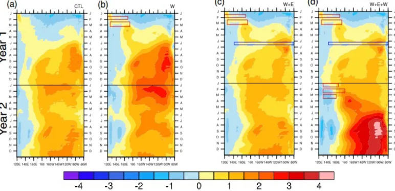
Observed total SST variance in Atl3 is characterised by a clear peak in May-July and a secondary peak in November- December (Fig. 1a). While STD fails to simulate this variance distribution, FLX is able to produce a summer variance peak in July-August. The delay in peak variance in FLX is in agreement with the delayed onset of the cold tongue.

To assess how dynamical processes contribute to total SST variance in Atl3, we decompose SST variance into a dynamically driven and a stochastically forced component.

The canonical approach for such a decomposition is to equate the ensemble mean of a simulation with the dynamical contribution to a signal. The observed climate record, however, corresponds to a single realisation of a climate simulation and does not allow for such a simple decomposition.

Our alternative decomposition approach uses empirical models of dynamical SST with multiple predictors. We base our choice of SST predictors on processes in the coupled equatorial ocean-atmosphere system that have a demonstrated impact on SST: The (i) thermocline and (ii) zonal advection feedbacks both support the growth of SST anomalies and are in turn related to the Bjerknes feedback (Bjerknes, 1969). We represent these feedbacks by our predictors of dynamical SST: (i) Sea surface height (SSH) is strongly related to the equatorial thermocline depth and upper ocean heat content and is our stand- in for the thermocline feedback. (ii) Zonal surface wind anomalies (u10) are related to zonal surface current anomalies and hence to the zonal advection feedback.

We estimate the parameters of our empirical models of dynamical SST via least-squares fitting of SSH and u10 to SST. All variables are used in their anomaly form. We build separate models for observations (ERA-Interim/AVISO) and the two KCM experiments (FLX, STD). Note that for our empirical models based on the KCM experiments, we use observed u10 instead of model u10. The reason is that our KCM experiments are partially coupled: The ocean does not "see“ the modeled, but observed wind stress anomalies. For each ensemble member and calendar month, we build a separate empirical model. We identify the response of our empirical model to our two predictor variables SSH and u10 as dynamical SST. Stochastic SST is the difference between the dynamical SST and the full SST (anomaly) that we used to build our empirical models with. Dynamical and stochastic SST variances are obtained as follows: For observations, we compute the variance of the two SST datasets for each calendar month. For the model experiments, we concatenate the (dynamical and stochastic SST) data for each calendar month from all ensemble members, and then compute the variance of the extended SST time series.

When we compare our empirical SST variance decomp-

osition approach with the ensemble-averaging approach for our two experiments, we find that it is a valid approximation.

Results: Impact of a realistic background state on the strength of dynamical SST variance

Figs. 1b,c show the dynamical and stochastic SST variances from our empirical model for Atl3. The ratio of the two variances is shown in Fig. 1d.

Observations: Observed dynamical SST clearly dominates SST variance during early boreal summer (May-July, Fig.

1b, black line). Dynamical SST variance then is roughly 4-7 times larger than the stochastic contribution to total SST variability (Fig. 1c). A secondary peak occurs during October and November. These two periods of enhanced dynamical SST variability are separated by phases during which stochastic SST variance is larger than dynamical SST variance. This is the case in January-March and again in August, when dynamical SST variance vanishes and observed stochastic SST variance reaches its peak. Note that observed stochastic SST variance is much less variable over the course of the year (Fig. 1c). This implies that stochastic SST variance is indeed driven by processes that are independent of seasonal processes — it represents noise. Lastly, comparing (observed) dynamical SST variance with total (observed) SST variance (Figs. 1a,b) shows a generally good agreement. This suggests that the (observed) seasonal cycle of total SST variability in Atl3 is largely shaped by the variable dynamical contribution.

Model simulations: FLX dynamical and stochastic SST variances are comparable to observations (blue).

Dynamical SST variance peaks in boreal summer and again, more weakly, in early boreal winter (Fig. 1b).

However, the timing of the dynamical SST variance peaks does not match observations: The summer peak lags Figure 1: Atl3 seasonal cycle of (a) total variance, (b) dynamical variance, (c) stochastic variance, and (d) the ratio of dynamical and stochastic variance, for (black, blue, red) ERA-Interim/AVISO, FLX, and STD. Note that the total STD variance in (a) is not shown completely due to y-axis scaling.

The missing values for January and February are 0.67 and 0.58°C², respectively.