based modular detector cluster for the MAGIC telescopes

based modular detector cluster for the MAGIC telescopes

Wissenschaftliche Arbeit zur Erlangung des Grades M.Sc.

an der Fakultät für Physik der Technischen Universität München.

Betreut von Prof. Dr. Elisa Resconi

Experimental Physics with Cosmic Particles

Eingereicht von Alexander Hahn Gutenbergweg 24 84034 Landshut +49 871 682 33

Eingereicht am München, den 03.04.2017

Gene Kranz, former NASA Flight Director

Abstract

MAGIC is a system of two imaging atmospheric Cherenkov telescopes (IACTs) dedicated to high energy gamma-ray observations. The telescopes are located at the Observatorio del Roque de los Muchachos on the Canary island of La Palma at 2200 m above sea level. Both telescope cameras are currently equipped with 1039 photomultiplier tubes (PMTs), each. The design of the MAGIC cameras offers the great possibility to test new light detectors alongside the existing camera. I participated in the development of a silicon photomultiplier (SiPM) based detector module. Its purpose is to evaluate the potential of SiPMs for existing and future IACTs.

To be considered as a possible replacement of PMTs, SiPMs need to overcome their restriction of small active areas. Therefore we combined SiPMs to a composite matrix in order to achieve the same active area as the 1-inch PMTs currently in use. The first SiPM module prototype, con- sisting of seven pixels was installed in the MAGIC camera in May 2015. It is integrated into the standard data taking and is operated alongside the PMT camera.

During the design process we addressed special constraints like the high level of background light and the angular acceptance of semiconductor photo sensors.

I integrated the SiPM module slow control to the existing standard software and developed calib-

ration procedures based on the charge spectrum of dark counts.

MAGIC ist ein System bestehend aus zwei abbildenden Tscherenkow-Teleskopen die der Beo- bachtung von hochenergetischen Gammastrahlen gewidmet sind. Die Teleskope befinden sich im Observatorio del Roque de los Muchachos auf der Kanarischen Insel La Palma, in einer Höhe von 2200m über dem Meeresspiegel. Beide Teleskopkameras sind derzeit mit jeweils 1039 Pho- toelektronenvervielfachern (PMTs) ausgestattet. Das Design der MAGIC-Kameras eröffnet die großartige Möglichkeit Module bestehend aus neuen Lichtdetektoren neben der vorhanden Kam- era zu testen. Ich habe an der Entwicklung eines aus Silizium-Photomultipliern bestehenden De- tektormoduls mitgewirkt. Sein Zweck ist es die Möglichkeiten von SiPMs in bereits vorhanden und neuen Tscherenkow-Teleskopen zu erforschen.

Um als Alternative in Betracht gezogen zu werden müssen SiPMs ihre Beschränkung auf kleine aktive Flächen überwinden. Hierfür kombinierten wir SiPMs zu einer Matrix um die selbe aktive Fläche zu erreichen wie sie die derzeitigen ein Zoll PMTs haben. Der erste Prototyp, bestehend aus sieben Pixeln, wurde im Mai 2015 in der MAGIC Kamera installiert. Er ist in die normale Datennahme eingebunden und wird neben der bereits vorhandenen PMT-Kamera betrieben.

Während der Konstruktion berücksichtigten wir Randbedingungen wie das hohe Hintergrundlicht und die winkelabhängige Akzeptanz der Halbleitersensoren.

Ich band die Steuerung diese Moduls in die vorhandene Steuersoftware ein und entwickelte eine

Kalibrierungsmethode, basierend auf dem Ladungsspektrum von Dunkelpulsen.

Contents

1 Introduction ... 1

1.1 Astroparticle Physics... 1

1.1.1 Extensive Air Showers ... 3

1.1.2 γ -ray Astronomy ... 5

1.2 Imaging Atmospheric Cherenkov Telescopes ... 9

1.3 The MAGIC Telescopes ... 10

1.4 Light Sensors ... 14

1.4.1 Eye ... 14

1.4.2 Photographic Emulsion ... 14

1.4.3 CCD ... 15

1.4.4 CMOS... 15

1.4.5 PIN Photodiode and APD ... 16

1.4.6 PMT ... 17

1.4.7 HPD... 18

1.4.8 SiPM... 18

2 Development of the SiPM Detector Module ... 21

2.1 Motivation for Building a SiPM based Detector Module... 21

2.2 Constraints of the Project... 22

2.3 Chosen Photosensors... 23

2.3.1 Excelitas SiPM ... 23

2.3.2 Expected Performance... 27

2.4 Light Guide Simulations ... 29

2.4.1 Requirements on the Light Concentrators ... 29

2.4.2 Simulations ... 32

2.4.3 Final Design... 35

2.4.4 Measurements ... 36

2.5 Cluster Design... 43

2.5.1 Pixel ... 43

2.5.2 High Voltage Supply ... 44

2.5.3 SiPM Bias Voltage ... 47

2.5.4 Summation ... 48

2.5.5 Optical signal transmission ... 49

2.5.6 Pulse Injection... 50

2.5.7 Slow Control PCB ... 51

2.6 Slow Control ... 51

3.2 Installation in La Palma ... 57

4 Results ... 60

4.1 Calibration Procedure... 60

4.2 Stability... 64

4.3 Comparison with PMTs... 65

5 Summary ... 69

6 Outlook ... 70

6.1 Further Ideas on the Calibration... 70

6.2 Second Generation SiPM Clusters ... 71

7 Publications and Presentations at Conferences ... 73

8 Appendix ... 75

List of Figures ... 88

List of Acronyms ... 91

List of Tables ... 94

Bibliography ... 95

Acknowledgements ... 103

1.1. Astroparticle Physics

Astroparticle physics is a young branch of particle physics. Its aim is to study elementary particles of astronomical origin to reveal properties of their sources and cosmology by combining astro- nomy, astro-, particle-, and detector-physics.

Cosmic rays are high-energetic particles that constantly interact with the Earth’s atmosphere. In 1910 Theodor Wulf measured an additional radiation component coming ”from the atmosphere (in German)” when he climbed the Eiffel Tower [105]. Two years later Victor Hess measured an increase of ionizing radiation at high altitudes and thereby discovered cosmic rays by concluding that ”there is a radiation from above penetrating the atmosphere (in German)” [59].

In 1929 Bothe and Kolhörster measured this ”corpuscular” (in German, consisting of discrete particles) radiation using Geiger-Müller counters in coincidence mode. They concluded that the energy of the particles has to be more than 1 GeV and speculated that the acceleration in space could happen in very extended electro-magnetic fields [21].

Nowadays this radiation is called primary cosmic rays. It consists of 85 % protons, 12 % Helium nuclei and 2 % electrons [48, 67]. The all-particle cosmic ray spectrum is plotted in figure 1. It covers 13 orders of magnitude in energy and 31 orders of magnitude in flux. The first labelled spectral softening is called knee. Protons with energies higher than 10

eV are not confined by the galactic magnetic field causing the softening of the spectrum [66]. Another possible explan- ation is the limited acceleration of particles by supernovae [16]. The flattening of the spectrum above 10

eV (the so-called ankle) might be caused by extragalactic particles. At even higher energies (> 6 × 10

eV) cosmic rays (predominantly protons) will interact with the cosmic mi- crowave background (CMB):

p + γ

→ p + π

, n + π

(1.1)

This reaction is causing a suppression in the spectrum for particles of distant sources. It is com- monly referred to as the Greisen-Zatsepin-Kuzmin (GZK) cutoff [47, 108].

Only very view primary cosmic rays reach the Earth’s surface. That is because the particles

interact with the earth’s atmosphere so that only secondary particles can reach the ground. The

high energetic particles generate an extensive air shower at their reaction with the air molecules

in the Earth’s atmosphere. After the first interaction more and more particles are created until

the particles lost too much energy to produce new particles. At this point the particle cascade

is gradually stopping. This shower propagates in longitudinal but also in lateral direction. Air

1 Introduction

showers of hadronic primary particles show a much higher lateral extension than electromagnetic showers induced by photons or electrons. The lateral extension can be seen in figure 2.

Energy (eV) LEAP

Proton AKENO KASCADE Auger SD Auger hybrid AGASA

HiRes-I monocular HiRes-II monocular

Knee

Ankle

10²

10^–1

10^–4

10^–7

10^–10

10^–13

10^–16

10^–19

10^–22

10^–25

10^–28

Fl u x (m

sr s G ev )

10⁹ 10¹⁰ 10¹¹ 10¹² 10¹³ 10¹⁴ 10¹⁵ 10¹⁶ 10¹⁷ 10¹⁸ 10¹⁹ 10²⁰ 10²¹

Figure 1

All-particle spectrum of cosmic rays [16]

1.1.1. Extensive Air Showers

The existence of extensive air showers was proven by Pierre Auger in 1938/1939 (in French [11, 12], in English [10]). They can be divided into two classes: hadronic air showers and elec- tromagnetic air showers.

5 km

5 km

5 km

5 km

a) c)

b) d)

Figure 2

Monte Carlo simulations of extensive air showers for

primary particles. a) and b) show a longitudinal and the lateral projection of the particle tracks for an incident photon. c) and d) show the same projections for a proton as primary particle in the same scale. Particle tracks of electrons, positrons, and gammas are plotted in red; Muon tracks in green; and hadronic tracks in blue. [92]

Hadronic air showers consist of three different components pictured in figure 2. The first com-

ponent is the hadronic component. It is the core component of the air shower. It provides the

electromagnetic component primarily via neutral pion decays through π

→ γγ. Each high-

energetic photon then creates an electromagnetic subshower. Charged pions and kaons contribute

1 Introduction

to the muonic air shower component [41].

Electromagnetic air showers are not only subshowers of hadronic showers but are also created by incident gamma photons hitting the Earth’s atmosphere. The primary photon undergoes pair pro- duction in the presence of the nucleons in the atmosphere. The produced electrons and positrons emit high energy photons via bremsstrahlung. These two processes are repeated alternately un- til the energy of each shower particle undercuts the critical energy of ≈ 81 MeV. Below this threshold photons lose their energy primarily through ionization [81]. A schematic diagram of the two different air shower processes is shown in figure 3.

e+

e+

e- primaryγ

e–

e+

e+ e+ e–

e–

e–

e– e– e+ e+ +

π+ π–

+- K , etc.

nucleons,

+- K , etc.

nucleons,

π0

π⁺ π⁰

µ^– _ γ

γ

µ

γ γ

νµ

νµ cosmic ray (p,α, Fe ...)

γ γ

γ γ

atmospheric nucleus

EM shower EM shower

EM shower atmospheric nucleus

Figure 3

Diagram of electromagnetic (left) and hadronic (right) extended air showers [100].

Charged primary particles are deflected in the cosmic magnetic fields during their travel to the

Earth. This causes the particle flux to be isotropic at energies below 10

eV. Information on

individual sources can only be gained by observing neutrinos or photons. The Earth’s atmosphere

permits only well defined windows in the electromagnetic spectrum where observations with

ground based telescopes are possible. Figure 4 shows these atmospheric windows as well as the

suitable instruments for measuring in them. The optical astronomy is the classical way to observe

celestial objects and systematically done for thousands of years but only exploits a very narrow

window in the electromagnetic spectrum [63].

40 km 20 km

100km γ

HE

N2, O2, O3, O H2O CO2

EAS

10⁶m 1 Mm 10³m 1 km 10^-3m

1 mm 10^-9m

1 nm 10^-12m 1 pm 1 am

10^-18m

1 mµ 10^-6m 10^-15m

1 fm

1 m

radio eV 1 eV

IR UV 1 keV 1 MeV

300 GHz 300 kHz 300 MHz eV

1 mm

1 EeV

18 1 PeV eV 10¹⁵

1 TeV eV 10¹²

1 GeV eV

10⁹ 10⁶eV 10³eV 10^-3eV 10^-6eV 10^-9eV 10^-12eV 10^-15 10

VHE X

UHE visible

Cosmic microwave background, ~3 mm

γ-rays

satellites

radio telescopes optical

telescopes balloons rockets

Cherenkov telescopes fluorescence

detectors

50% of incident radiation absorbed

particle detectors

Earth surface

Figure 4

Atmospheric windows used in astronomy [100].

1.1.2. γ -ray Astronomy

Nowadays all wavelength of the electromagnetic spectrum are exploited ranging from radio and infrared waveband, over the visible spectrum to beyond X-ray observations. A relatively new field of astronomy is the γ-ray astronomy focused on the highest energetic photons up to teraelectron- volts. But also photons do not reach the Earth undistorted. They can be deflected by gravitational lensing or absorbed by interaction (pair production) with other photons (CMB, infrared, X-ray, or visible) [62]. This not only evokes many interesting phenomena to study but also mechanisms one has to take into account when studying γ -ray production. The production mechanisms of γ-rays are synchrotron radiation of accelerated electrons in a magnetic field, bremsstrahlung, and inverse Compton scattering of X-rays on high energy electrons. If protons are accelerated in a source they can produce neutral pions by proton-proton interaction for example. These neutral pions emit two photons in their decay like the neutral pions in extensive air showers. It is theoretically feasible that also matter-antimatter annihilations, dark matter decay or the annihilation of hypothetical neutralinos could produce γ-rays. Currently there are many theories trying to explain the leptonic or hadronic processes that can the accelerate particles to such high energies to produce high ener- getic γ -rays. Measuring these γ -rays helps understanding the physics of the acceleration sites and particle physics at energies unprecedented at artificial accelerators. γ-ray astronomy is of high importance for this understanding. Despite the low count rate at these energies, sources can emit half of their energy through γ-rays. If one would not take them into account one would ignore a significant part of the source characteristics.

Hadronic showers are background to γ-ray astronomy measurements. Because hadronic showers

are many orders of magnitude more frequent, a good separation between hadronic and electro-

magnetic showers is necessary. Hadronic showers form much deeper in the atmosphere due to

1 Introduction

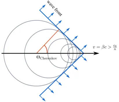
Θ

w av e front

v = βc >

Figure 5

Illustration of the Cherenkov light creation by an ultrarelativistic charged particle (phase velocity

with refractive index

the small cross-section of hadrons. Multiple scattering, electromagnetic subshowers from neut- ral pion decay, and high transverse momentum transfer lead to a broadened and more irregular particle cascade.

The relativistic secondary particles of the air shower emit Cherenkov light if their phase speed v is higher than the speed of light in air v =

with c the speed of light in vacuum and n the refractive index of the medium. The charged particle electrically polarizes the dielectric medium (air in this case) while propagating through it. Due to the limited relaxation speed of the medium, the energy contained in this polarization is then coherently radiated. Cherenkov light is emitted under a well defined angle given by equation 1.2 [25].

Θ

= arccos c nv

= arccos 1

nβ

with n the refractive index of the propagation medium and c the speed of light in vacuum.

(1.2)

The number of Cherenkov photons a particle produces along its track is given by equation 1.3

[81].

d

N

dE dx = αz

¯

hc sin

(Θ

)

= α

z

r

m

c

1 − 1 β

n

(E)

(1.3)

≈ 370 sin

Θ

(E)

eV

cm

with α the fine-structure constant and n as the refractive index function of photon energy E.

From equation 1.3 it follows that the intensity of Cherenkov light is proportional to the refractive index n. At low altitudes where the density of air is higher, more Cherenkov photons will be produced. The Cherenkov light produced by electrons and positrons at an altitude of 10 km is emitted under an angle of 0.8

[41]. At 2200 m altitude the Cherenkov angle is increased to 1.2

because of the higher air density [13]. Each particle of the electromagnetic shower with a high enough energy is therefore illuminating a ring on the ground. These rings overlap and form a characteristic, circular photon distribution on the ground as can be seen in figure 6. Within

Density of Cherenk o v photons ( m

) 18 16 14 12 10 8 6 4 2

0 0 50 100 150 200 250 300

Distance to shower core (m) Shower core

Figure 6

Cherenkov photon distribution on the ground at 2220 m altitude created by a

until where mostly core photons can be observed is marked by a green line. Adaptecd from [13].

a radius of roughly 120 m for vertical showers, the photon distribution can be described as an

almost flat distribution where the Cherenkov photon density is directly proportional to the energy

of the primary γ-ray (see figure 7). The typical photon density within the core radius of 120 m

is 100 photons m

TeV

[61]. The photon distribution on the ground can be parameterized by

1 Introduction

[38]:

C(r) =



 

 

 

 

C

e

if 30 m < r ≤ 120 m C

if 120 m < r ≤ 350 m

with C

as normalization parameter, s the exponential slope in the core region, and power law index k.

One can see a prominent hump at the cores inner border before the rapid decrease above 120 m.

This feature is caused by the altitude depending refractive index of air. This causes an almost constant product of height h and Cherenkov angle Θ

. In addition the emission of Cher- enkov light increases with the refractive index as described above. These two effects cause the hump for γ-rays from about 100 GeV to several tens of TeV [85]. The average photon density for shower core photons for different primary particles is plotted in figure 7. One can easily see that the atmosphere acts as an almost ideal calorimeter for primary γ-rays, converting a fixed fraction of the primary’s energy to Cherenkov light. From this it follows that the energy of the primary can be reconstructed by measuring the Cherenkov intensity on the ground. It has to be mentioned that this dim Cherenkov flashes have a duration of only a few nano seconds [5].

Photon Density ( m

)

Energy (GeV)

10

10

10

γ

p He

N

Mg

Fe 10

10

10

1

10

10

constant

fraction

Figure 7

Cherenkov photon yield plotted as average density for shower core photons for different primary particles. Only photons

between

to

arriving within the first

are taken into account. Adapted from [80].

1.2. Imaging Atmospheric Cherenkov Telescopes

In 1953 the first Cherenkov light emitting air showers were detected by Galbraith and Jelley after it was already predicted by Blackett in 1948. Their detector consisted of a parabolic mirror with a single photomultiplier tube (PMT) mounted in the focal point. The mirror and the light detector were mounted inside a garbage can to shield the detector from stray light. For coincidence meas- urements they used an array of 16 Geiger-Müller counters surrounding the garbage can [43].

This technique was further improved by increasing the mirror size and the number of PMTs in the focal plane. This newborn air Cherenkov technique had the advantage of a higher precision in energy estimation and angular resolution compared to air shower arrays because the full shower development can be recorded [35].

Yet all Cherenkov telescopes used only one or very few PMTs as photo sensors including the 10 meter Whipple telescope constructed in 1968. This made it impossible for all telescopes in that time to distinguish between electromagnetic and hadronic air showers. The Whipple camera was upgraded to an imaging camera with 37 PMTs in 1983. This upgrade made it possible to separate electromagnetic from hadronic showers because astronomers did no longer rely on the measure- ment of a count rate but were able to count events of a certain type. The analysis was significantly improved by Hillas with the invention of the parameterization of the shower images in 1985 [60].

Thereby detecting the first source for γ -rays, the Crab Nebula [102].

Today Imaging Atmospheric Cherenkov Telescopes (IACTs) are able to detect showers induced by particles with their primary energy between ∼ 30 GeV to tens of TeV. By combining the informations from two or more telescopes in coincidence mode the reconstruction of the charac- teristics of the primary particles (kind, energy, and direction) can be further improved. An illustra- tion of stereo observations can be found in figure 8. The air shower is recorded by two telescopes.

Both camera images are then parametrized and combined to reconstruct the particles original

direction and energy. Currently there are three major IACTs in operation: Major Atmospheric

Gamma Imaging Cherenkov (MAGIC), Very Energetic Radiation Imaging Telescope Array Sys-

tem (VERITAS), and High Energy Stereoscopic System (H.E.S.S.). They will be substituted in

the future by the Cherenkov Telescope Array (CTA), parts are currently under construction. All

three existing and the future Large Size Telescopes (LSTs) of CTA use cameras based on PMTs

[6, 20, 42, 84].

1 Introduction

20

km

10

Figure 8

Stereo observations with an IACT. The Cherenkov photons of an extensive air shower are focused to the camera by the parabolic mirrors. The characteristic image of events is drawn next to the telescopes. The Hillas parameterization is indicated by the ellipse and the axis drawn to the events. The superposition of the events of both telescopes provides a precise reconstruction of the primary particle’s properties. Adapted from [39, 62].

1.3. The MAGIC Telescopes

After having discussions on "a major atmospheric cerenkov detector" already in 1992, the MAGIC collaboration was formally formed in 1998 [37]. Today this international collaboration consists of about 160 scientists from 24 institutions in 11 counties.

The construction phase of the first telescope was finished in 2003 and scientific operation star- ted the year after. In 2009 the second telescope was added to provide stereoscopic views on the extended air showers. This allows three-dimensional air shower impact point and direction re- construction, improving the angular and energy resolution. During regular observations, the two telescopes are operated in coincidence mode which fosters the background rejection and there- fore lowers the energy threshold. In 2012, the upgrade of readout electronics and the first MAGIC camera was finished. Since this upgrade both telescopes are nearly identical.

The two MAGIC IACTs are set up on the Canary island of La Palma in the Atlantic ocean (see

Fig.9). They are located at the Observatorio del Roque de los Muchachos (ORM) at an altitude

of about 2200 m a.s.l. . The night sky of this site is protected by a unique law, regulating light-,

radioelectrical-, and atmospheric pollution as well as aviation routes [32]. Because the ORM is

becoming one of the host sites of CTA, the first LST is currently being built next to MAGIC.

The former High-Energy-Gamma-Ray Astronomy (HEGRA) experiment was also located at this site.

Figure 9

The Canary archipelago and the African coast photographed from the ISS [31]. The MAGIC telescopes are located on the island of La Palma which can be identified on the bottom left in this image.

Figure 10

The two MAGIC telescopes on the Canary island of La Palma as seen from the Swedish solar telescope. The experiment is located at the ORM at an altitude of

The telescopes are dedicated to observations of very high energy γ -rays in an energy range from

∼ 50 GeV to more than 50 TeV originating from galactic and extragalactic sources [7].

The telescopes MAGIC-1 and MAGIC-2 are 85 m apart from each other as shown figure 10. Both

parabolic reflector dishes have a diameter of 17 m consisting of 247 individual mirrors. All mir-

rors can be adjusted by an active mirror control. This allows compensating for the bending of the

telescopes at different observation zenith angles. A picture of the mirror dish can be found in the

1 Introduction

appendix figure 69.

Most of the telescope structures is made of reinforced carbon fibre tubes. This makes the tele- scopes with less than 70 tons very light. Due to this light weight construction both telescopes can be rotated fast (7

s

) and can reach any point in the sky within 20 s. A fast reposition- ing is of high importance for gamma-ray burst (GRB) observations. A drawing of the structure construction can be seen in figure 11.

8500 8500

300

18816 22458

16295

11134 264 270

17000 17264 28134

10600

Figure 11

CAD drawing of the MAGIC-1 telescope. Dimensions are given in

Both cameras are equipped with 1039 PMTs partitioned in 169 so called clusters. Each cluster consists of up to seven photo sensors with high voltage supply, amplifier, and optical signal con- verter. The clusters at the camera edge are not fully equipped to provide the circular detection area. In the six corners of the housing’s hexagon shape an additional cluster can be placed as shown in figure 12. The field of view (FoV) of the telescope is 3.5

. Each PMT is topped with

Figure 12

The camera of the MAGIC-2 telescope. On the right hand side the six free corners of the telescope’s camera are indicated

in green. Adapted from [76].

a light concentrator which is increasing the active area of the PMTs. This hollow light guide is made of a plastic structure with a glued metallized Mylar foil inside. A more detailed explanation follows in section 2.4.

Controlling and data acquisition are situated in the counting house next to the telescopes. The analog electronic signal of a pixel is converted to an analog optical pulse by a fibre coupled vertical-cavity surface-emitting laser (VCSEL). A short explanation of the working principle of a VCSEL and fibre couplings can be found in the book by Meschede [73]. This optical analog pulse is then received at the counting house and digitized by a Domino Ring Sampler version 4 (DRS4) based readout [90]. MAGIC saves the unprocessed raw data of an event in form of the digitized waveform with a speed of 1.64 Gsps, corresponding to a snapshot of the signal’s amp- litude every 0.6 ns. While consuming a lot of disk space this has the advantage that special data processing can be applied offline. This is utilized especially for trigger and new detector module developments.

The trigger is a threshold trigger based on the sum of next neighbour pixels. Only an inner circle of 547 PMTs is taken into account. This corresponds to a trigger area of 4.30 deg

. To reduce spurious events triggered by the light of the night sky (LoNS) the telescopes are operated in coin- cidence mode. A stereo triggered event consists of 50 samples taken with the sampling frequency of 1.64 GHz which results in about 30 ns per event. The readout can handle trigger frequencies of up to 1 kHz with a fixed dead time after a trigger of 26 µs after every recorded event.

By using a sliding window peak search algorithm the charge is extracted from the waveform data in the standard analysis [107].

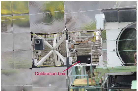
For the calibration of the PMTs a light flasher is installed at the centre of the mirror dish in a so-

called calibration box. This box houses a fast pulsed frequency tripled Nd:YAG laser with 355 nm

and ∼ 700 ps pulse width (STV-01E-150 from Soliton) [97]. The beam can be attenuated by two

remote controlled consecutive filter wheels before entering an Ulbricht sphere. The light exits the

integrating sphere towards the camera in order to homogeneously illuminate it. The calibration

box produces flashes at a fixed frequency of 25 Hz during data taking in order to monitor possible

gain variations in the signal chain.

1 Introduction

Figure 13

Calibration box installed in the centre of the mirror dish. It consists of a Nd:YAG laser with a wavelength of

attenuation filters and an integrating sphere. Several small cameras which are monitoring the PMT camera and its surrounding can be seen. On the right hand side one can see the reflection of the open camera.

1.4. Light Sensors

There is a large variety of photo detectors available on the market. Before the actual development of a detector module can start one has to decide on a suitable low light level (LLL) sensor.

1.4.1. Eye

The history of photo sensors starts with the evolution of eyes, photochemical light sensors, about 500 - 600 million years ago. It all began with only dark and bright differencing cells containing protein pigments, continuously developing till it reached today’s form of colour vision eyes [45].

The resolution of human and animal eyes is high enough to sense single photons [15, 57]. Since a conscious response to single photons would lead to a too high noise rate, our brain employs an integration filter on our vision. Only if five to eight photons within 100 − 150 ms are received a conscious perception is generated [57, 82]. One problem in spotting the UV to blue Cherenkov showers by naked eye is the transmittance of the lens (aquula). It shows a sharp cut-off towards shorter wavelength at around 400 nm [19]. Due to this fact and for a precise quantification humans need to use artificial detectors to record Cherenkov showers.

1.4.2. Photographic Emulsion

Another light detector based on photochemical reactions is photographic emulsion. It was ex-

cessively used in particle physics in form of films or photo plates. For example cloud and bubble

chamber events were recorded on special photographic films for later analysis. Nowadays bubble

and cloud chambers are obsolete but until the mid 1980’s tens of millions of photographs were taken and analysed [58]. They enabled physicists to detect several new particles at that time for example the first detection of a positron and a muon [35].

Photographic emulsion was also used as a direct particle detector in the Direct Observation of the Nu Tau (DONUT) and the Oscillation Project with Emulsion-tRacking Apparatus (OPERA) experiments [29, 77].

Photographic emulsion is more sensitive in the blue and UV regions. Silver iodine has a sensitivity maximum at 423 nm for instance. Nevertheless, the photographic emulsion is not very suitable for detecting low light levels due to its low sensitivity which requires thousands or millions of photons to achieve enough contrast in the image [72].

1.4.3. CCD

Widely used are charge-coupled device (CCD) sensors. They are imaging sensors in which the charge-coupled, light sensitive but individual pixels provide position sensitive information on the flux of light. The generated electrical charge in each pixel is stepwise moved through the sensor to the readout. A full readout cycle is completed after the charge of all pixels has been moved to the analog-to-digital converters (ADCs). This takes some time, so even with high technical effort the mean frame rate is in the order of hundreds of micro seconds [26]. In the time between the readout cycles the incident light is integrated in the pixels. CCDs are sensitive over a wide spectral range from UV to infrared, peaking in green and offer a high detection efficiency. In 2009 the Nobel Prize for Physics was awarded for the invention of the CCD concept back in 1969. There is heavy use of CCDs in astronomy and astrophysics. The Gaia mission of the European space agency (ESA) for instance, uses 106 individual CCDs totalling almost a billion pixels [83]. In order to reduce thermal noise (thermally excited electrons) most CCDs are cooled. For lab experiments operating temperatures of − 50

C are typical but for high precision applications liquid gases can be used for further cooling. Due to the long integration times CCDs are not suitable for the detection of Cherenkov showers.

1.4.4. CMOS

In the 1990s an different pixellated photo sensor was developed at the JPL (Jet Propulsion Labor- atory) of NASA (National Aeronautics and Space Administration): The so called complementary metal–oxide–semiconductor (CMOS) sensor. The name of the sensor refers to the technology for constructing the integrated circuits. They consist of individual pixels made up of a photodiode and some transistors for switching the reverse bias and signal voltages. The photodiode is initially charged by a known fixed voltage and then disconnected from the bias supply. During illumina- tion the photoinduced charge separation lowers this voltage. At readout this remaining voltages is directly measured without the need of shifting the charges (contrary to CCDs) to the readout first.

All switching and readout electronics can be placed on the same dice which makes this sensor

type very cheap. In addition it is possible to pack colour sensitive pixels much denser on CMOSs

as on CCDs. Due to these facts CMOS sensors are the dominant imaging sensor type in consumer

1 Introduction

electronics and are gaining importance in scientific applications [44]. The necessity of additional circuitry around the pixels leads to lower sensor fill factor which reduces the quantum efficiency of a CMOS sensors compared to CCDs. Lately the minimal possible acquisition time dropped below 1 µs per image [30]. This is still too slow compared to the duration of the light flashes from extended air showers (see section 1.2). The wide spectral sensitivity with its maximum in the near infra-red (NIR) would lead to a worsened signal-to-noise ratio because the LoNS is increasing to- wards longer wavelength (see section 2.2).

In addition to the described too low speed, mismatching sensitivities, and high technical effort there is no additional information gained by using an imaging device coupled to a non-imaging light guide. One would need to equip the full camera plane with expensive CCD or CMOS sensors. Altogether I summarize that CCDs and CMOS sensors are not suited for air shower detection in IACTs. Although especially CCDs might be used for gaining additional information for example on the pointing by imaging starts in the FoV.

1.4.5. PIN Photodiode and APD

A photo detector known since the 1960s is the positive intrinsic negative (PIN) photodiode. It is still used in high energy physics experiments for the readout of scintillating crystals. Another practical example is the use for simple monitoring of light sources. As all pure solid state light detectors they are insensitive to magnetic fields and are rather compact. Nevertheless it is not possible to use PIN photodiodes in IACTs because they require between 200 - 300 photons for a detectable signal and their peak sensitivity is in the red to infrared region. An additional drawback for their application is the low bandwidth of just a few 100 kHz.

The avalanche photodiode (APD) is a further development of PIN photodiodes. In contrast to PIN diodes, an APD has an intrinsic gain and much lower noise while providing sensitivity down to tens of photons. After the incoming photon created a free electron via internal photo effect, the free electron is accelerated in the p-n junction and creates more electron-hole pairs by im- pact ionization. This process is repeated several times thus achieving an internal gain of typically 50 to 200. With a p-on-n layer structure sensitivity is highest for blue light. Their temperature dependence is very high even for indirect semiconductor based photo sensors. Because they are operated in the linear gain regime below the breakdown voltage, the temperature has to be stable within a fraction of a degree. This was realized for the Compact Muon Solenoid (CMS) experi- ment which uses APDs in the electromagnetic calorimeter. It requires the sensor temperature to be stable within ± 0.05

C to preserve the energy resolution [23]. This of course is impractical for the usage in telescopes which are operated at changing ambient temperatures.

The APD was followed by the development of single photon sensitive devices as for example the

visible-light photon counter (VLPC), superconducting nanowire single-photon detector (SNSPD),

and transition edge sensor (TES). The common disadvantage of all these sensor types is the oper-

ation at cryogenic temperatures of a few Kelvin which rules them out for the desired use.

1.4.6. PMT

The photomultiplier tube (PMT) was developed in 1930 by Leonid Kubetsky and is nowadays widely used in astronomy, medical imaging, and high energy physics [65].

It consists of a vacuum tube with a multi-dynode stage inside. The photo cathode is supplied with a high voltage (∼ 1000 V) which is shared with the dynodes via a resistive voltage divider. A schematic view is shown in figure 14. An incident photon creates a free electron via photoelec- tric effect at the photo cathode. This so called photo-electron (ph.e) is then accelerated in the electric potential towards the first dynode. Focusing electrodes can be used optionally to increase the collection efficiency of this first dynode. The accelerated electron releases a bunch of new electrons at impact at the dynode. This bunch of electrons is again accelerated towards the next dynode where the process of secondary emission repeats for each electron of the bunch thereby amplifying the signal at each dynode. After several dynodes PMTs can reach a gain of 10

− 10

while still being able to resolve single photo-electrons [87]. PMTs can be manufactured with very different active area sizes. Small and compact PMTs are for example used in hand-held radiation detectors whereas huge PMTs with a size of 550 cm

are used by the IceCube Neutrino Observat- ory and even bigger ones with 2400 cm

in the Super-Kamioka Neutrino Detection Experiment [1, 40, 54–56].

Photo cathode

Dynodes

Photo-electron Photon

Anode

Figure 14

Schematic view of a PMT.

The PMT’s overall photon detection efficiency is strongly dependent on material used as photo cathode, its thickness, and on the mentioned collection efficiency of the first dynode. Today’s PMTs used for the LSTs of CTA reach a quantum efficiency (QE) of 43 % [71]. John Smedley’s (Brookhaven National Laboratory) latest research on photo cathodes might give hope that the QE could be further improved in the future [96].

Because the first free electron is accelerated in vacuum its trajectory strongly depends on the

surrounding magnetic field. The PMTs in the MAGIC cameras are therefore shielded with a

mu-metal wrapping against disturbances. Ageing effects might reduce the detection efficiency

with time by lowering the conversion efficiency of the photo cathode or destruction of the dynode

coating. Powered PMTs show accelerated ageing until destruction when exposed to bright light

and therefore need to be protected against high photon currents. Because the photo-electrons need

to travel different distances from the photo cathode to the first dynode depending on the point of

interaction of the incoming photon, there is a time spread in the outgoing signal. This so-called

1 Introduction

transit time spread (TTS), is gain dependent and usually in the order of several ns [75].

PMTs provide very fast signal shape with a width of a just few ns. The conversion of ADC counts to photo-electrons is very easy by using the so-called F-factor method which was described by Mirzoyan and Schweizer in [74] and [94].

The spectral sensitivity of borosilicate glass window PMTs matches very nicely the Cherenkov spectrum while being less sensitive to the LoNS [75].

1.4.7. HPD

The hybrid photo detector (HPD) is a spin-off of the PMT. It has the same photo cathode for conversion of photons to free electrons but instead of the dynode structure an APD is used inside the vacuum housing. It is operated at a high voltage of 6 − 8 kV. The impinging photo-electrons create electron hole pairs inside the silicon. The electron hole pairs are accelerated in the ava- lanche region of the APD and release an additional avalanche. Both effects provide a combined amplification of 10

− 10

[87]. HPDs can resolve single photo-electrons very clearly while keeping the fast signal shape and high bandwidth of PMTs. Because of their construction HPDs are sensitive to magnetic fields and need to be operated at stable temperatures. They are a few times more expensive compared to PMTs and there are not as many different sizes available as for PMTs. MAGIC currently uses only one HPD for measuring the atmospheric transmission with a Lidar (Light detection and ranging) system [39]. But wavelength shifter coated HPDs were considered for an upgrade of a MAGIC camera in recent years [91].

1.4.8. SiPM

If the bias voltage of an APD is increased one eventually reaches the breakdown voltage where also the holes are accelerated enough to create new electron hole pairs. Both charge carriers con- tribute now to the avalanche which is therefore self-sustaining. This mode of operation is called Geiger-mode. To stop this avalanche the bias voltage needs to be lowered under the breakdown voltage. After stopping the avalanche the APD needs to re-charge and is then able to trigger an- other time. This is only practicable at low trigger rates and cryogenic temperatures otherwise the thermally excited dark counts would saturate the APD without any external light. One can how- ever divide the APD into a array of individual small APDs. The resulting device is called a silicon photomultiplier (SiPM). The individual APD cells are again biased with a common voltage above the breakdown and are therefore called Geiger-mode APDs (G-APDs). Photons can only be de- tected at the active are of each cell. The space between the cells, used for biasing the cells and shielding cross talk is field free and therefore dead. A simplified drawing of the layer structure of a SiPM can be found in figure 15. It shows the metal contact for biasing the cell and the trenches between the cells to prevent cross-talk. Cross-talk is caused by photons emitted from the charge avalanche at brake down. The emitted photons can reach a neighbouring cell an trigger a break- down in this cell. The output signal indistinguishable from the real detection of two photons.

Therefore the cross-talk plays an important role in the reconstruction of the number of incident

photons from the measured signal.

There are many other names for this device like: multi-pixel Geiger-mode avalanche photodiodes (MAPD), solid-state photomultipliers (SSPM), discrete amplification photon detector (DAPD), pixelated photon detector (PPD) but SiPM is slowly ousting the other names. Sometimes G-APD was used to refer to the full sensor instead of only a single cell. Throughout this work the above- mentioned definitions of SiPM as the device and G-APD as a single cell of this device will be used.

While a regular APD has a big capacitance and therefore a long recharge time after breakdown, SiPM cells are much smaller and therefore have much smaller recharge times. Standard cell sizes or better cell pitches are 50 µm, 75 µm and 100 µm. The number off cells is giving the dynamic range but on the other hand the dead area is increasing with the number of cells as well.

Each G-APD gives an identical signal when being triggered. At low light levels the information from each cell can be considered as a binary: cell fired or not fired. The consequence is that SiPMs have an extraordinary good charge resolution which is superior to the one of PMTs and HPDs [86].

Because of the use of silicon, which is an indirect band gap semiconductor, SiPMs show a tem- perature dependent gain. Even in absence of light, thermally excited electrons can trigger a break- down. Due to the binary nature of the cell’s signal, there is no way to distinguish them from real light induced signals.

One of the advantages of SiPMs is their compactness and their low operation voltage which is

usually between 25 V and 100 V. The spectral sensitivity of SiPMs ranges from 350 − 900 nm

which makes them suitable for air shower detection but one must keep in mind that more LoNS

than with a PMT will be collected as well.

1 Introduction

Metal contact

n+

p

avalanche region n

Photon

SiO

n

n+

Trech Epoxy

Avalanche

Figure 15

Structure of a SiPM. The incident photon passes the protective

layer and creates an electron hole pair in the p-n-junction, shown in the top right. Trenches for cross-talk suppression can be seen. The device is covered by a protective Epoxy layer. The cells are biased via the metal contacts on the top and covered by an anti-reflective

layer.

As outlined above, and based on the integration time, photo detection efficiency, temperature and

wavelength dependency, it is evident tha out of the presented possibilities only PMTs, HPDs, and

SiPMs are suitable for the utilisation in IACTs.

2.1. Motivation for Building a SiPM based Detector Module

Many astroparticle physics experiments rely on the detection of light. Cherenkov flashes are targeted by IACTs and neutrino detectors like IceCube or KM3Net [2, 3]. Other experiments like the Pierre Auger Observatory observe fluorescence light in the atmosphere [98]. Light detectors are also used for the readout of scintillating fibres or crystals for example in the Antiproton Flux in Space (AFIS) mission or the Large Area Telescope (LAT) of the Fermi Gamma-ray Space Telescope (Fermi) [9, 68].

Current PMT based cameras of IACTs cannot be operated during full moon periods because of too much background light. SiPMs however are resistant to a high amount of background illumination. Utilizing SiPMs as a light detector for MAGIC could therefore increase the duty cycle by allowing operation during moon and twilight times from 18 % (dark nights only) to 40 % [49, 89]. As an alternative, there are tests undergoing to protect the PMT camera with an UV-pass filter during full moon.

The figure of merit for IACTs is the energy threshold. A low energy threshold is necessary to be able to study phenomena like GRBs and extragalactic background light (EBL) absorption.

IACTs can lower their threshold by collecting more photons from an air shower by increasing their mirror size. However, this is limited because large telescopes become very expensive and complicated in construction. Another possibility to get more photons from an air shower is by increasing the photon detection efficiency (PDE) of the used sensors. SiPMs are rather new and are still improved steadily and therefore might be used in future IACT cameras.

The First G-APD Cherenkov Telescope (FACT) uses already SiPMs for several years. It has proven that small pixel size IACTs consisting of SiPMs are possible to construct and operate.

FACT uses a separate readout channel for each of their 1440 SiPMs [64]. Such a fine pixelization is neither necessary nor useful for the MAGIC or the future LST cameras. Instead, several SiPMs need to be combined to form a composite pixel with the same size as a PMT.

This work will focus on the joining of several SiPMs to a combined IACT light detector module which is a novel approach to enhance our instrument’s performance.

SiPM modules (also called SiPM cluster) can be installed in a MAGIC camera next to the PMT

modules. Both types of sensors will be operated alongside to provide a fair, real live comparison

under real observation conditions.

2 Development of the SiPM Detector Module

2.2. Constraints of the Project

In order to be able to mount the SiPM module to the desired MAGIC 1 camera many constraints have to be addressed.

The most obvious one is the mechanical form factor of our new cluster. The camera front with the light guides is protected by a Poly(methyl methacrylate) (PMMA) window and inside the camera two cooling plates comprise the main mechanical structure holding all detector modules of the camera. A cut-away view is drawn in figure 16. This is a proven camera design and the future CTA LST is based on it [27]. The SiPM module has to fit into the form factor of the standard PMT cluster which therefore defines the maximal width and length. Additionally we must consider the radiated electronic noise, produced heat and available electricity.

The project’s aim is to compose several SiPMs to reach the same active area as a PMT. Therefore the individual pixels of this SiPM module should have the same size as the hemispherical 1 inch PMTs currently used in the MAGIC-1 camera.

Figure 16

Cut-away view of the MAGIC camera structure. At the front the PMMA window can be seen. At the camera rear the opposite removed camera cover can be seen. [103]

The readout of the MAGIC telescopes is situated in the counting house as described in section 1.3. We will use the same readout for recording the data from the SiPM cluster. This allows us a direct comparison between PMT and SiPM modules.

For transmitting the signals to the counting house the same optical transmission line will be used.

That implies we have to convert the analog electronic pixel output to an analog optical pulse. To

be able to record the SiPM data in the readout the signal amplitudes must be similar to the one of

a PMT pixel. Taking this transmission line into account leads to an amplitude of about

as pixel output.

The SiPM module needs different slow control mechanisms with respect to a PMT module. It would be possible to set up a dedicated software but it is more convenient for the shift crew if the SiPM functionalities are embedded to the standard camera control (CaCo).

2.3. Chosen Photosensors

For this project the C30742-66-050-X SiPMs from Excelitas technologies were chosen. Excelitas is an US American company with an SiPM production facility in Canada. It is currently owned by the private equity firm Veritas Capital Management L.L.C. [33, 99].

2.3.1. Excelitas SiPM

Excelitas uses a P-on-N semiconductor structure for their short wavelength sensitive SiPMs. The basic structure is explained in figure 15. The C30742-66-050-X SiPM (figure 17) has an active area of 6 × 6 mm

with a cell pitch of 50 µm. This results in a total of 14400 cells [34]. The typical bias voltage is around 100 V − 105 V where a gain of 1.5 × 10

will be reached.

The expected dark count rate is several 10 MHz but because the light of the night sky (LoNS) will induce a rate of several 100 MHz they do not need to be concerned further for this study.

The so called fill factor, the ratio of dead to active area of the SiPM was not provided by Excelitas so I measured it using a Keyence VHX-5000 microscope. One of the obtained images is shown in figure 18. When measuring the active area of a cell A

one has to subtract the dead area of the metal contacts. The fill factor F F can be calculated with equation 2.1 by dividing the active area per cell A

times total cell count N

by the total area A

. This is equivalent to dividing the active area per cell by the cell pitch A

. The fill factor was found to be 47 %.

FF = A

× N

A

≡ A

A

(2.1)

= A

50 × 50 µm

= 47 %

The cross-talk plays a key role for the calibration of the SiPM cluster once it is installed in the MAGIC camera. To determine the cell cross-talk of the SiPMs I compared three different methods in our laboratory beforehand.

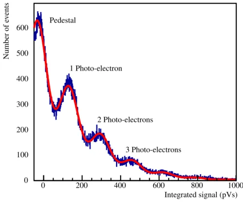
For the first method the single photo-electron spectrum is fitted with a parameterized spectrum function of correlated Gauss peaks distributed according to a Poisson distribution (see figure 19).

The cross-talk is causing a deviation from the pure Poission distribution and can therefore be

2 Development of the SiPM Detector Module

1 mm

Figure 17

Excelitas C30742-66-050-X SiPM.

35.19 µm

100 µm 2016/04/12

Lens: Z500:X2000

35.36 µm

Additional dead area 49.71 µm

Figure 18

Close-up view of the Excelitas SiPM at 2000x magnification. The individual cell area was measured as well as the area of

the metal contacts of each cell to calculate the fill factor.

Integrated signal (pVs)

0 200 400 600 800 1000

Number of ev ents

0 100 200 300 400 500 600

Pedestal

1 Photo-electron

2 Photo-electrons

3 Photo-electrons

Figure 19

Cross-talk determination by a single photo-electron spectrum fit.

directly determined from the function. This is a very reliable method as the fit function converges even for not fully separated single photo-electron peaks. When the SiPM cluster is operated in the MAGIC camera this method cannot be used because the sliding window peak search signal extraction algorithm introduces a strong but different bias on each photo-electron peak which the fit function can not account for. It is therefore used as the reference method in this laboratory comparison shown in figure 21.

The second method is similarly based on the cross-talk caused mismatch of the data and a pure Poisson distribution. First the distance D of the photo-electron peaks at positions x

is determ- ined. Then all events between x

−

and x

+

are integrated. The resulting histogram in units of photo-electrons (shown in figure 20) is then compared to a fitted Poisson distribution.

The cross-talk probability P

is calculated as the normalized difference of the expected number of events according to the Poisson distribution N

and the recorded single photo- electron events N

:

P

= N

− N

N

(2.2) This method shows large uncertainties at low bias voltages. At low gain the photo-electron peaks are overlapping and the integration of the peak areas is very error prone. The determined cross- talk probabilities using this method are plotted in figure 21 in green.

A third method uses the inherently existing dark counts. Events recorded with a random trig-

ger should only show either no signals or signals from single photo-electrons. With cross-talk

2 Development of the SiPM Detector Module

Number of photo-electrons

0 2 4 6 8 10

Poisson distribution Fraction Data

10 -3 10 -2 10 -1

1

Figure 20

Cross-talk determination by comparison of the integrated single photo-electron spectrum to a Poisson distribution at the level of one photo-electron.

however there will be a number of events showing two or more photo-electrons because the breakdown cell has triggered a nearby cell at the same time. The cross-talk probability can be calculated using the number of the recorded cross-talk events with showing two or more photo- electrons N

and the number of recorded dark counts, which is the number of events with one or more photo-electrons N

:

P

= N

N

(2.3) This method can only be used at higher bias voltages with separated photo-electron peaks. Oth- erwise it is not possible to define ranges for the event histogram integration. The benefit of this method is that it can be used without concerning the bias caused by the sliding window peak search algorithm in the MAGIC data analysis.

At room temperature the dark count rate of a SiPM is in the order of a few MHz. The probability of two dark counts occurring at the same time P (≥ 2)

can be calculated with equation 2.4 with DCR the dark count rate and τ the width of the integration window.

P (≥ 2)

= 1 − [P(1)

+ P (0)

]

= 1 −

(DCR · τ )

· e

1! + (DCR · τ )

· e

0!

= 1 − e

· (1 − DCR · τ ) (2.4)

With the precise knowledge of the dark count rate at the given bias voltage and temperature one could apply corrections for this probability as I demonstrated in my bachelor thesis [51]. This would be very impractical during operation of the SiPM cluster inside the MAGIC camera. So for the comparison of the different cross-talk determination methods no correction is needed here and the result of equation 2.4 is used as an additional uncertainty contribution of about 1 %.

The cross-talk determined with equation 2.3 is shown in figure 21 in red.

Figure 21

Comparison of three different cross-talk measurement methods. The cross-talk probabilities determined with a single photo-electron spectrum fit function are shown in blue. This fit offers the most reliable method over the full bias voltage range. In green the cross-talk probability determined by a comparison of measured data to a Poisson distribution is plotted. At low bias voltages this method only give unreliable values. The red graph shows the most simple method of determining the cross-talk probability. It uses only the number of events per photo-electron peak. This method works with the randomly occurring dark counts and is immune to biases introduced by the signal extraction algorithms.

In figure 21 one can see that the Poisson distribution method shows a systematic offset compared to the spectrum fitting method. The simple method of integrating the single photo-electron peaks shows the largest uncertainties but is comparable to the other two methods. For the operation of our SiPM module we will use the latter method because we do not need a precise cross-talk determination and we can profit from the benefit of this third method, i.e. the analysis of the dark counts.

2.3.2. Expected Performance

To estimate the performance of our SiPM light detector module I compared the spectral efficiency (PDE (λ)) curves of the PMTs used in the MAGIC-1 camera with the efficiency of the Excelitas SiPMs. In figure 22 the towards longer wavelength extended sensitivity of a SiPM can be seen.

It does not match the Cherenkov spectrum as good as the PMT sensitivity. It is evident that the

2 Development of the SiPM Detector Module

SiPM pixels will detect less Cherenkov photons while being more sensitive to the LoNS.

For a quantitative comparison it is necessary to do a pointwise multiplication (equations 2.5 and 2.6) of the efficiency of a given sensor with the LoNS spectrum S

or the air Cherenkov spectrum S

. The resulting graphs are also shown in figure 22.

(PDE · S

) (λ) = PDE (λ) · S

(λ) (2.5) (PDE · S

) (λ) = PDE (λ) · S

(λ) (2.6)

Wavelength (nm)

200 300 400 500 600 700 800 900

Ef ficienc y (%)

120

0 1000 20 40 60 80 100

Photon count (a.u.)

LoNS spectrum SiPM PDE PMT QE

Convolved LoNS spectrum (SiPM) Convolved LoNS spectrum (PMT) Cherenkov spectrum

Figure 22

LoNS spectrum at the MAGIC site and efficiencies of the Excelitas SiPMs and the Hamamatsu PMT currently used MAGIC camera [56]. The sensor responses are shown by the pointwise multiplication of the sensors efficiency with the LoNS spectrum. Additionally the Cherenkov spectrum of an extended air shower for low zenith observations is plotted. The Cherenkov spectrum is based on measurements from [28] in the range from

to

and on monte carlo simulations for

to

By comparing the integrals of the PMT and SiPM responses we can estimate that the SiPM pixel will detect 57 % less Cherenkov photons of a gamma event. Concomitantly a 4.3 times higher noise rate will be induced by the LoNS in a SiPM pixel. It follows that the signal to noise ratio of this first prototype will be one tens with respect to the PMT pixel. This can be seen as a conservat- ive estimate because the mirror response, the losses in the plexi glass and the collection efficiency of the PMT is not yet taken into account. The Cherenkov spectrum used for this estimation is for low zenith angle observations only, for inclined showers the maximum of the Cherenkov spec- trum shifts to longer wavelength, which would increase the signal to noise ratio of SiPM pixels.

The single photo-electron rate of a PMT pixel induced by the LoNS is unknown for the current

configuration of the MAGIC telescopes. However the first MAGIC camera showed a LoNS rate

of 130 MHz [14]. Because the peak QE of the PMTs increased from 26 % to 34 % (31 % relative)

with the camera upgrade, I conservatively assume a 40 % increase of the LoNS rate for the cur- rent configuration. Because of the extended red sensitivity of SiPMs the same LoNS will produce photo-electrons at a rate of 780 MHz in a SiPM pixel. The full width at half maximum (FWHM) of a SiPM single photo-electron signal is about 5 ns. This means that we will have pileup effects which will make it impossible to distinguish single photo-electrons during observations.

Divided by the number of cells of a SiPM and the number of SiPMs I estimate a rate of 7.76 kHz per cell. The function of exponential re-charge of a SiPM cell is defined by the time constant τ . It can be calculated from the value of the quenching resistor R

times the cell capacitance C

:

V (t) = V

· 1 − e

t Rq·Ccell

= V

·

1 − e

with τ = R

· C

(2.7)

It follows that a cell will be re-charged to 99 % after about 437 ns. Using the estimated LoNS rate as the expectation value of a Poisson distribution I calculated a probability of only 0.34 % that a cell will be triggered again before it is re-charged. Both functions are shown in figure 23. This means that we can assume a constant gain during dark time observations.

Time(µs) 0 0.05 0.1 0.15 0.2 0.25 0.3

Char ge (%)

0 10 20 30 40 50 60 70 80 90 100

T rigger pr obability (%)

0.2 0.6 0.8 1

0 0.35 0.4 0.45 0.5

0.4

Figure 23

SiPM re-charge and probability for a LoNS induced trigger.

2.4. Light Guide Simulations

2.4.1. Requirements on the Light Concentrators

In all IACTs light concentrators are used to increase the active area of the telescope camera and to

define the acceptance of each light sensor. It is sufficient to use non-imaging light concentrators

because the PMT and SiPM pixels are non-imaging as well. Combining information from indi-

vidual pixels one obtains an image. Typically, cameras of modern IACTs consist of 500 - 1000