Biogeochemical protocols and diagnostics for the CMIP6 Ocean Model Intercomparison Project (OMIP)

(1)

https://doi.org/10.5194/gmd-10-2169-2017

Biogeochemical protocols and diagnostics for the CMIP6 Ocean Model Intercomparison Project (OMIP)

James C. Orr¹, Raymond G. Najjar², Olivier Aumont³, Laurent Bopp¹, John L. Bullister⁴, Gokhan Danabasoglu⁵, Scott C. Doney⁶, John P. Dunne⁷, Jean-Claude Dutay¹, Heather Graven⁸, Stephen M. Griffies⁷, Jasmin G. John⁷, Fortunat Joos⁹, Ingeborg Levin¹⁰, Keith Lindsay⁵, Richard J. Matear¹¹, Galen A. McKinley¹², Anne Mouchet^13,14, Andreas Oschlies¹⁵, Anastasia Romanou¹⁶, Reiner Schlitzer¹⁷, Alessandro Tagliabue¹⁸, Toste Tanhua¹⁵, and Andrew Yool¹⁹

1LSCE/IPSL, Laboratoire des Sciences du Climat et de l’Environnement, CEA-CNRS-UVSQ, Gif-sur-Yvette, France

2Dept. of Meteorology and Atmospheric Science, Pennsylvania State University, University Park, Pennsylvania, USA

3Laboratoire d’Océanographie et de Climatologie: Expérimentation et Approches Numériques, IPSL, Paris, France

4Pacific Marine Environmental Laboratory, NOAA, Seattle, Washington, USA

5National Center for Atmospheric Research, Boulder, Colorado, USA

6Marine Chemistry & Geochemistry, Woods Hole Oceanographic Institution, Woods Hole, Massachusetts, USA

7NOAA Geophysical Fluid Dynamics Laboratory, Princeton, New Jersey, USA

8Dept. of Physics, Imperial College, London, UK

9Climate and Environmental Physics, Physics Inst. & Oeschger Center for Climate Change Res., Univ. of Bern, Bern, Switzerland

10Institut fuer Umweltphysik, Universitaet Heidelberg, Heidelberg, Germany

11CSIRO Oceans and Atmosphere, Hobart, Tasmania 7000, Australia

12Atmospheric and Oceanic Sciences, University of Wisconsin-Madison, Madison, Wisconsin, USA

13Max Planck Institute for Meteorology, Hamburg, Germany

14Astrophysics, Geophysics and Oceanography Department, University of Liege, Liege, Belgium

15GEOMAR Helmholtz Centre for Ocean Research Kiel, Kiel, Germany

16Columbia University and NASA-Goddard Institute for Space Studies, New York, NY, USA

17Alfred Wegener Institute, Bremerhaven, Germany

18Earth, Ocean and Ecological Sciences, University of Liverpool, Liverpool, UK

19National Oceanographic Centre, Southampton, UK Correspondence to:James C. Orr (james.orr@lsce.ipsl.fr) Received: 20 June 2016 – Discussion started: 18 July 2016

Revised: 28 February 2017 – Accepted: 7 March 2017 – Published: 9 June 2017

Abstract. The Ocean Model Intercomparison Project (OMIP) focuses on the physics and biogeochemistry of the ocean component of Earth system models participating in the sixth phase of the Coupled Model Intercomparison Project (CMIP6). OMIP aims to provide standard protocols and diagnostics for ocean models, while offering a forum to pro- mote their common assessment and improvement. It also offers to compare solutions of the same ocean models when forced with reanalysis data (OMIP simulations) vs. when integrated within fully coupled Earth system models (CMIP6).

Here we detail simulation protocols and diagnostics for OMIP’s biogeochemical and inert chemical tracers. These passive-tracer simulations will be coupled to ocean circulation models, initialized with observational data or output from a model spin-up, and forced by repeating the 1948–

2009 surface fluxes of heat, fresh water, and momentum.

These so-called OMIP-BGC simulations include three inert chemical tracers (CFC-11, CFC-12, SF₆) and biogeochemical tracers (e.g., dissolved inorganic carbon, carbon isotopes, alkalinity, nutrients, and oxygen). Modelers will use their

(2)

preferred prognostic BGC model but should follow common guidelines for gas exchange and carbonate chemistry. Sim- ulations include both natural and total carbon tracers. The required forced simulation (omip1) will be initialized with gridded observational climatologies. An optional forced simulation (omip1-spunup) will be initialized instead with BGC fields from a long model spin-up, preferably for 2000 years or more, and forced by repeating the same 62-year meteo- rological forcing. That optional run will also include abiotic tracers of total dissolved inorganic carbon and radiocarbon, C_T^abio and¹⁴C_T^abio, to assess deep-ocean ventilation and distinguish the role of physics vs. biology. These simulations will be forced by observed atmospheric histories of the three inert gases and CO2as well as carbon isotope ratios of CO2. OMIP-BGC simulation protocols are founded on those from previous phases of the Ocean Carbon-Cycle Model Intercomparison Project. They have been merged and updated to reflect improvements concerning gas exchange, carbonate chemistry, and new data for initial conditions and atmospheric gas histories. Code is provided to facilitate their implementation.

1 Introduction

Centralized efforts to compare numerical models with one another and with data commonly lead to model improvements and accelerated development. The fundamental need for model comparison is fully embraced in Phase 6 of the Coupled Model Intercomparison Project (CMIP6), an initia- tive that aims to compare Earth system models (ESMs) and their climate-model counterparts as well as their individual components. CMIP6 emphasizes common forcing and diagnostics through 21 dedicated model intercomparison projects (MIPs) under a common umbrella (Eyring et al., 2016). One of these MIPs is the Ocean Model Intercomparison Project (OMIP). OMIP focuses on comparison of global ocean models that couple circulation, sea ice, and optional biogeochemistry, which together make up the ocean components of the ESMs used within CMIP6. OMIP works along two coordinated branches focused on ocean circulation and sea ice (OMIP-Physics) and on biogeochemistry (OMIP-BGC). The former is described in a companion paper in this same issue (Griffies et al., 2016), while the latter is described here.

Groups that participate in OMIP will use different ocean biogeochemical models coupled to different ocean general circulation models (OGCMs). The skill of the latter in sim- ulating ocean circulation affects the ability of the former to simulate ocean biogeochemistry. Thus previous efforts to compare global-scale, ocean biogeochemical models have also strived to evaluate simulated patterns of ocean circulation. For instance, the Ocean Carbon-Cycle Model Intercom- parison Project (OCMIP) included efforts to assess simulated circulation along with simulated biogeochemistry. OCMIP

began in 1995 as an effort to identify the principal differences between existing ocean carbon-cycle models. Its first phase (OCMIP1) included four models and focused on natural and anthropogenic components of oceanic carbon and radiocarbon (Sarmiento et al., 2000; Orr et al., 2001). OCMIP2 was launched in 1998, comparing 12 models with common biogeochemistry, and evaluating them with physical and inert chemical tracers (Doney et al., 2004; Dutay et al., 2002, 2004; Matsumoto et al., 2004; Orr et al., 2005; Najjar et al., 2007). In 2002, OCMIP3 turned its attention to evaluating simulated interannual variability in forced ocean biogeochemical models (e.g., Rodgers et al., 2004; Raynaud et al., 2006). More recently, OCMIP has focused on assessing ocean biogeochemistry simulated by ESMs (e.g., Bopp et al., 2013).

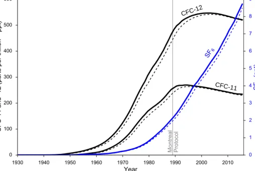
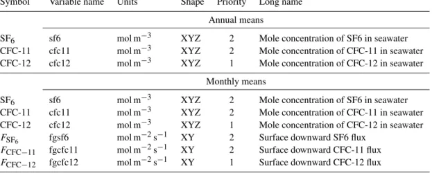
OCMIP2 evaluated simulated circulation using the phys- ically active tracers, temperature T and salinity S (Doney et al., 2004), but also with passive tracers, i.e., those having no effect on ocean circulation. For example, OCMIP2 used two anthropogenic transient tracers, CFC-11 and CFC- 12 (Dutay et al., 2002). Although these are reactive gases in the atmosphere that participate in the destruction of ozone, they remain inert once absorbed by the ocean. From an oceanographic perspective, they may be thought of as dye tracers given their inert nature and purely anthropogenic ori- gin, increasing only since the 1930s (Fig. 1). Furthermore, precise measurements of CFC-11 and CFC-12 have been made throughout the world ocean, e.g., having been col- lected extensively during WOCE (World Ocean Circulation Experiment) and CLIVAR (Climate and Ocean – Variabil- ity, Predictability and Change). Hence they are well suited for model evaluation and are particularly powerful when used together to deduce decadal ventilation times of sub- surface waters. Yet their combination is less useful to assess more recent ventilation, because their atmospheric concentrations have peaked and declined, since 1990 for CFC- 11 and since 2000 for CFC-12, as a result of the Montreal Protocol. To fill this recent gap, oceanographers now also measure SF₆, another anthropogenic, inert chemical tracer whose atmospheric concentration has increased nearly lin- early since the 1980s. Combining SF₆with either CFC-11 or CFC-12 is optimal for assessing even the most recent ventilation timescales. Together these inert chemical tracers can be used to assess transient time distributions. These TTDs are used to infer distributions of other passive tracer distributions, such as anthropogenic carbon (e.g., Waugh et al., 2003), which cannot be measured directly.

To help assess simulated circulation fields, OCMIP also included another passive tracer, radiocarbon, focusing on both its natural and anthropogenic components. Radiocar- bon (¹⁴C) is produced naturally by cosmogenic radiation in the atmosphere, invades the ocean via air–sea gas exchange, and is mixed into the deep sea. Its natural component is useful because its horizontal and vertical gradients in the deep ocean result not only from ocean transport but

(3)

1930 1940 1950 1960 1970 1980 1990 2000 2010

Year

0 100 200 300 400 500 600

CFC

11

and

12

(parts

per

trillion – ppt)

Montreal Protocol

CFC11 CFC12

SF⁶

0 1 2 3 4 5 6 7 8 9

SF6

(ppt)

Figure 1.Histories of annual-mean tropospheric mixing ratios of CFC-11, CFC-12, and SF₆for the Northern Hemisphere (solid line) and Southern Hemisphere (dashed line). Mixing ratios are given in parts per trillion (ppt) from mid-year data provided by Bullister (2015). For the OMIP simulations, these inert chemical tracers need not be included until the fourth CORE-II forcing cycle when they will be initialized to zero on 1 January 1936 (at model date 1 January 0237). The vertical grey line indicates the date when the Montreal protocol entered into force.

also from radioactive decay (half-life of 5700 years), leaving a time signature for the slow ventilation of the deep ocean (roughly 100 to 1000 years depending on location). Hence natural ¹⁴C provides rate information throughout the deep ocean, unlikeT andS. For example, the ventilation age of the deep North Pacific is about 1000 years, based on the de- pletion of its ¹⁴C/C ratio (−260 ‰ in terms of 1¹⁴C, i.e., the fractionation-corrected ratio relative to that of the preindustrial atmosphere) when compared with that of source waters from the surface Southern Ocean (−160 ‰) (Toggweiler et al., 1989a). In the same vein, ventilation times of North Atlantic Deep Water and Antarctic Bottom Water have been deduced from¹⁴C in combination with another biogeochemical tracer PO^∗₄(“phosphate star”) (Broecker et al., 1998) by taking advantage of their strong regional contrasts. The natural component of radiocarbon complements the three inert chemical tracers mentioned above, which are used to assess more recently ventilated waters nearer to the surface. Yet the natural component is only half of the story.

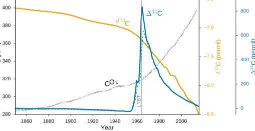
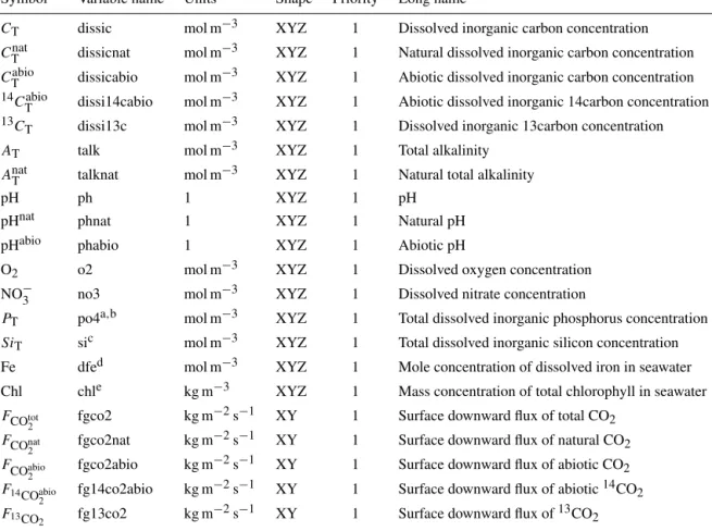
During the industrial era, atmospheric1¹⁴C declined due to emissions of fossil CO₂ (Suess effect) until the 1950s when that signal was overwhelmed by the much larger spike from atmospheric nuclear weapons tests (Fig. 2). Since the latter dominates, the total change from both anthropogenic effects is often referred to as bomb radiocarbon. As an anthropogenic transient tracer, bomb radiocarbon complements CFC-11, CFC-12, and SF₆ because of its different atmospheric history and much longer air–sea equilibration time

(Broecker and Peng, 1974). Observations of bomb radiocarbon have been used to constrain the global-mean gas transfer velocity (Broecker and Peng, 1982; Sweeney et al., 2007);

however, in recent decades, ocean radiocarbon changes have become more sensitive to interior transport and mixing, making it behave more like anthropogenic CO₂ (Graven et al., 2012). Hence it is particularly relevant to use radiocarbon observations to evaluate ocean carbon-cycle models that aim to assess uptake of anthropogenic carbon as done during OCMIP (e.g., Orr et al., 2001).

Information from the stable carbon isotope¹³C also helps to constrain the anthropogenic perturbation in dissolved inorganic carbon by exploiting the Suess effect (Quay et al., 1992, 2003). Driven by the release of anthropogenic CO₂ produced from agriculture, deforestation, and fossil-fuel combustion, the Suess effect has resulted in a continuing re- duction of the¹³C/¹²C ratio relative to that of the preindustrial atmosphere–ocean system. That ratio is reported relative to a standard asδ¹³C, which is not corrected for fractionation, unlike1¹⁴C. Fractionation occurs during gas exchange and photosynthesis, andδ¹³C is also sensitive to respiration of organic material and ocean mixing. Oceanδ¹³C observations have been used to test marine ecosystem models, including processes such as phytoplankton growth rate, iron limitation, and grazing (Schmittner et al., 2013; Tagliabue and Bopp, 2008) and may also provide insight into climate- related ecosystem changes. Past changes inδ¹³C recorded in

(4)

1860 1880 1900 1920 1940 1960 1980 2000

Year

280 300 320 340 360 380 400

CO2 (ppm)

CO

²

8.5 8.0 7.5 7.0 6.5

δ

13C (permil)

δ

¹³

_C

0 200 400 600 800

∆14C (permil)

∆

¹⁴

C

LTBT

Figure 2.Annual-mean atmospheric histories for global-mean CO₂(black dots) andδ¹³C (orange) compared to hemispheric means of1¹⁴C for the north (blue solid) and south (blue dashes). Isotope records are available at input4mips (https://esgf-node.llnl.gov/search/input4mips/), including tropical1¹⁴C (30^◦S–30^◦N) (not shown). The CO₂data are identical to those used for CMIP6 (Meinshausen et al., 2016) and the carbon isotope data are common with C4MIP (Jones et al., 2016). The CO₂observations are from NOAA (Dlugokencky and Tans, 2016). The δ¹³C compilation uses ice-core and atmospheric measurements (Rubino et al., 2013; Keeling et al., 2001), while the1¹⁴C compilation uses tree-ring and atmospheric measurements Levin et al. (2010), extended after 2009 with unpublished data from the University of Heidelberg (I. Levin, personal communication, 2016). Post-2009 data are not needed in OMIP Phase 1, but will be used in subsequent phases. Between the beginning of the OMIP simulations on 1 January 1700 and the same date in 1850, the atmospheric concentrations of CO₂,δ¹³C, and 1¹⁴C are to be held constant at 284.32 ppm, 6.8, and 0 ‰, respectively. Also indicated are the preindustrial reference (0 ‰) for atmospheric 1¹⁴C (horizontal grey dashed) and when the Limited Test Ban Treaty (LTBT) went into effect (vertical grey solid).

ice cores and marine sediments are likewise useful to evaluate models (Schmitt et al., 2012; Oliver et al., 2010).

Besides the aforementioned tracers to evaluate modeled circulation fields, OMIP-BGC also includes other passive tracers to compare simulated ocean biogeochemistry with data and among models, e.g., in terms of mean states, trends, and variability. Whereas all OCMIP2 groups used a common biogeochemical model (Najjar and Orr, 1998, 1999;

Najjar et al., 2007), essentially testing its sensitivity to different circulation fields, OMIP will not adopt the same approach. Rather, OMIP focuses on evaluating and comparing preselected “combined” ocean models (circulation- ice-biogeochemistry) largely defined already by individual groups planning to participate in CMIP6. Those combined ocean models will be evaluated when forced by reanalysis data as well as when coupled within the CMIP6 ESMs.

OMIP-BGC model groups will use common physical forcing for ocean-only models and common formulations for carbonate chemistry, gas exchange, gas solubilities, and Schmidt numbers. Biogeochemical models will be coupled to the ocean-ice physical models, online (active and passive tracers will be modeled simultaneously), and they will be forced with the same atmospheric gas histories. Yet beyond those commonalities, model groups are free to choose their preferred ocean model configuration. For instance, groups may choose whether or not to include direct coupling between simulated chlorophyll and ocean dynamics. When coupled, chlorophyll is not a typical passive tracer; it is ac-

tive in the sense that it affects ocean circulation. Likewise, OMIP groups are free to use their preferred boundary conditions for the different sources of nutrients and micronutrients to the ocean via atmospheric deposition, sediment mobiliza- tion, and hydrothermal sources (e.g., for Fe) as well as lat- eral input of carbon from river and groundwater discharge.

Biogeochemical models with riverine delivery of carbon and nutrients to the ocean usually include sediment deposition as well as loss of carbon from rivers back to the atmosphere through the air–sea exchange. Each group is free to use their preferred approach as long as mass is approximately con- served. Groups are requested to provide global integrals of these boundary conditions and to document their approach, preferably in a peer-reviewed publication.

OMIP-BGC aims to provide the technical foundation to assess trends, variability, and related uncertainties in ocean carbon and related biogeochemical variables since the onset of the industrial era and into the future. That foundation includes (1) the OMIP-BGC protocols for groups that will include inert chemical tracers and biogeochemistry in OMIP’s two forced global ocean model simulations, which couple circulation, sea ice, and biogeochemistry, and (2) the com- plete list of ocean biogeochemical diagnostics for OMIP, but also for CMIP6 (Eyring et al., 2016) and any ocean-related MIPs under its umbrella, e.g., C4MIP (Jones et al., 2016).

Simulated results from OMIP-BGC will be exploited to contribute to OMIP’s effort to study basic CMIP6 science questions on the origins and consequences of systematic

(5)

model biases. In particular, OMIP-BGC offers a forum for ocean biogeochemical modelers and a technical framework by which they will assess and improve biases of simulated tracer and biogeochemical components of CMIP6’s ESMs.

OMIP-BGC will contribute to the World Climate Research Programme’s (WCRP) Grand Challenges by providing fundamental information needed to improve near-term climate prediction and estimates of carbon feedbacks in the climate system. Assessments will focus on current and future changes in ocean carbon uptake and storage, acidification, deoxygenation, and changes in marine productivity.

Novel analyses are expected from OMIP, in part because of recent improvements in the physical and biogeochemical components. For example, some of the physical models will have sufficient resolution to partially resolve mesoscale ed- dies. When coupled to biogeochemical models, that combination should allow OMIP to provide a first assessment of how air–sea CO₂fluxes and related biogeochemical variables are affected by the ocean’s intrinsic variability (also known as internal, chaotic, or unforced variability). Previous studies of the ocean’s internal variability have focused only on physical variables (Penduff et al., 2011). Other studies have as- sessed the internal variability of ocean biogeochemistry, but they account only for the component associated with turbu- lence in the atmosphere. That is, they use a coarse-resolution ocean model coupled within an Earth system model framework (Lovenduski et al., 2016). Whether internal variability from the ocean works to enhance or reduce that from the atmosphere will depend on the variable studied, the region, and the model. OMIP aims to provide new insight into the ocean’s contribution to internal variability while also quanti- fying the relative importance of the contribution of internal variability to the overall uncertainty of model projections.

2 Protocols

As described by Griffies et al. (2016), the OMIP-Physics simulations consist of forcing physical model systems (an ocean general circulation model coupled to a sea-ice model) with the interannually varying atmospheric data reanalysis known as the Coordinated Ocean-ice Reference Experiments (CORE-II) available over 1948–2009 (Large and Yeager, 2009). For OMIP, that 62-year forcing will be repeated five times to make simulations of 310 years. OMIP-BGC participants will make these simulations by coupling their prognostic models of ocean biogeochemistry, online, to their physical model systems. These OMIP-BGC simulations will be forced by observed records of atmospheric CO₂ and other gases during the 310-year period, defined as equivalent to calendar years 1700 to 2009. One 310-year OMIP simulation (omip1), with models initialized by data, is required (Tier 1) for all OMIP modeling groups; another 310-year simulation (omip1-spunup), with models initialized from a previous long spin-up simulation, is only for OMIP-BGC groups. Al-

though optional, theomip1-spunupsimulation is strongly encouraged (Tier 2) to minimize drift, assess deep-ocean ventilation, and separate physical vs. biological components of ocean carbon. Details of these simulations are provided below.

The two forced ocean model simulations, omip1 and omip1-spunup, differ from but are connected to the CMIP6 DECK and historical simulations. The only differences are the initialization and the forcing. Inomip1, the ocean model is initialized with observations and forced by reanalysis data;

inhistorical, the ocean model is coupled within an Earth system model framework after some type of spin-up. Likewise, the early portion of theomip1-spunupforced simulation is comparable to the CMIP6 DECKpiControlcoupled simulation. The complementarity of approaches will lead to a more thorough model evaluation.

When modeling chemical and biogeochemical tracers, it is recommended that OMIP groups use the same formulations for gas exchange and carbonate chemistry as outlined below. Little effort would be needed to modify code that is already consistent with previous phases of OCMIP. For gas exchange, model groups only need to change the value of the gas transfer coefficient, the formulations and coefficients for Schmidt numbers, and the atmospheric gas histories. For carbonate chemistry, groups should strive to use the constants recommended for best practices (Dickson et al., 2007) on the total pH scale and to avoid common modeling assumptions that lead to significant biases, notably an oversimplified alkalinity equation (Orr and Epitalon, 2015). Fortran 95 code to make these calculations is made available to OMIP-BGC participants.

2.1 Passive tracers 2.1.1 Inert chemistry

The inert chemistry component of OMIP includes online simulation of CFC-11, CFC-12, and SF₆. While CFC-12 is required (priority 1), CFC-11 and SF₆ are encouraged (priority 2). About the same amount of observational data in the global ocean exists for both CFC-11 and CFC-12, starting with early field programs in the 1980s. But CFC-12 has a longer atmospheric history, with its production starting a decade earlier (∼1936) and a slower decline starting a decade later due to its longer atmospheric lifetime (112 vs.

52 years) relative to CFC-11 (Rigby et al., 2013). In contrast, SF₆has continued to increase rapidly in recent decades.

That increase will continue for many years despite ongo- ing efforts to restrict production and release of this potent greenhouse gas, because SF₆’s atmospheric lifetime is per- haps 3000 years (Montzka et al., 2003). Using pairs of these tracers offers a powerful means to constrain ventilation ages;

if model groups are only able to model two of these tracers, the ideal combination is CFC-12 and SF₆.

(6)

Simulation protocols are based on the OCMIP2 design document (Najjar and Orr, 1998) and its ensuing CFC protocol (Orr et al., 1999a) and model comparison (Dutay et al., 2002). These inert passive tracers are computed online along with the active tracers (i.e., temperature and salinity in the physical simulation); they are independent of the biogeochemical model. OMIP models will be forced to follow historical atmospheric concentrations of CFC-11, CFC-12, and SF₆, accounting for gas exchange and their different solubilities and Schmidt numbers. The same passive tracers should be included in the forced OMIP simulations and in the coupled CMIP6 historical simulations. Both types of simulations will be analyzed within the framework of OMIP.

These inert chemistry tracers are complementary to the ideal age tracer that is included in the OMIP-Physics protocols (Griffies et al., 2016).

2.1.2 Biogeochemistry

For the other passive tracers, referred to as biogeochemistry, the OMIP-BGC protocols build on those developed for OCMIP. These include the OCMIP2 abiotic and biotic protocols (Najjar and Orr, 1998, 1999; Orr et al., 1999b) and the OCMIP3 protocols for interannually forced simulations (Au- mont et al., 2004), all available online with links to code and data (see references) or as one combined PDF (see Supple- ment). Each model group will implement the OMIP protocol in their own prognostic ocean biogeochemical model as in OCMIP3, unlike the common-model approach of OCMIP2.

Each OMIP biogeochemical model will be coupled online to an ocean general circulation model forced by the CORE-II atmospheric state. Geochemical boundary conditions for the atmosphere include an imposed constant atmospheric concentration of O₂(mole fractionx_O₂of 0.20946) but a variable atmospheric CO₂ that follows observations (Meinshausen et al., 2016).

In addition, OMIP-BGC simulations should include a natural carbon tracer that sees a constant atmospheric mole fraction of CO₂ in dry air (x_CO₂) fixed at the 1 January 1850 value (284.32 ppm), the CMIP6 preindustrial reference. This can be done either in an independent simulation with identical initial conditions and forcing, except for atmospheric xCO₂, or in the same simulation by adding one or more new tracers to the biogeochemical model, referred to here as a dual-CT simulation. For thisdual simulation, OMIP modelers would need to add a second dissolved inorganic carbon tracer (C_T^nat), e.g., as in Yool et al. (2010). In OMIP, this added tracer will isolate natural CO₂and keep track of model drift. Suchdoublingmay also be necessary for other biogeochemical model tracers if they are directly affected by the CO₂increase. For instance, expansion of the PISCES model (Aumont and Bopp, 2006) to adual-C_Timplementation resulted in doubling not only ofC_T, but also of its transported CaCO₃tracer, which in turn affects total alkalinityA_T(Du- four et al., 2013). These natural tracers are referred to as

C_T^nat, CaCO^nat₃ , and A^nat_T . Calculated variables affected by CO₂ should also be doubled, including pH,pCO₂, the air–

sea CO₂flux, and carbonate ion concentration. If biology depends on CO₂, additional tracers such as nutrients and O₂ would also need to be doubled, making the doubling strategy less appealing. That strategy may also be more complex in some ESMs, e.g., ifA_Tchanges abiotically due to warming- related changes in weathering and river runoff.

2.1.3 Abiotic carbon and radiocarbon

In theomip1-spunupsimulation (as well as in its previously run spin-up) OMIP-BGC groups will also include two abiotic tracers to simulate total dissolved inorganic carbonC_Tâbioand corresponding radiocarbon¹⁴C_Tâbio. These abiotic tracers do not depend on any biotic tracers. They should be included in addition to the biotic carbon tracers mentioned above (C_T andC_T^nat). The ratio of the two abiotic tracers will be used to evaluate and compare models in terms of deep-ocean ventilation ages (natural radiocarbon) and near-surface anthropogenic invasion of bomb radiocarbon. In addition,C_Tâbiowill be compared toC_Tto distinguish physical from biogeochemical effects on total carbon. For simplicity, simulations will be made abiotically following OCMIP2 protocols (Orr et al., 1999b). We recommend that participating groups add these two independent tracers to their biogeochemical model to simulate them simultaneously, thus promoting internal consistency while reducing costs.

In OMIP, we will use this two-tracer approach rather than the simpler approach of modeling only the¹⁴C/C ratio directly (Toggweiler et al., 1989a, b). That simpler approach would be a better choice if our focus were only on comparing simulated and field-based estimates of the ocean’s bomb-¹⁴C inventory, both of which are biased low (Naegler, 2009; Mouchet, 2013). The simpler modeling approach un- derestimates the inventory, because it assumes a constant air–

sea CO₂ disequilibrium during the industrial era; likewise, field reconstructions of the ocean’s bomb-¹⁴C inventory (Key et al., 2004; Peacock, 2004; Sweeney et al., 2007) are biased low because they assume that oceanC_T is unaffected by the anthropogenic perturbation. Yet in terms of oceanic 1¹⁴C, the simple and two-tracer approaches yield similar results (Mouchet, 2013), because the effect of increasingCTon oceanic1¹⁴C is negligible (Naegler, 2009). We also choose the two-tracer approach to take advantage of itsC^abio_T tracer to help distinguish physical from biological contributions to CT.

To model ¹⁴C, OMIP neglects effects due to fractionation (i.e., from biology and gas exchange). Hence model results will be directly comparable to measurements reported as 1¹⁴C, a transformation of the¹⁴C/C ratio designed to correct for fractionation (Toggweiler et al., 1989a). Thus biases associated with our abiotic approach may generally be neglected. For natural¹⁴C, Bacastow and Maier-Reimer (1990) found essentially identical results for simulations that

(7)

accounted for biological fractionation vs. those that did not, as long as the atmospheric CO₂ boundary conditions were identical. For bomb ¹⁴C, which also includes the Suess effect, neglecting biological fractionation results in small biases (Joos et al., 1997).

Hence for the omip1-spunup simulation, OMIP-BGC groups will simulate four flavors of dissolved inorganic carbon: biotic natural (C_T^nat), biotic total (C_T), abiotic total (C_T^abio), and abiotic radiocarbon (¹⁴C_T^abio). Conversely for the omip1simulation, groups will simulate only the first two flavors,C_T^nat andCT. These tracers may be simulated simultaneously or in separate simulations, although we recommend the former.

2.1.4 Carbon-13

Groups that have experience modeling¹³C in their biogeochemical model are requested to include it as a tracer in the OMIP-BGC simulations. Groups without experience should avoid adding it. It is not required to simulate ¹³C in order to participate in OMIP. Modeling groups that will simulate ocean¹³C are requested to report net air–sea fluxes of¹³CO₂ and concentrations of total dissolved inorganic carbon-13 (¹³CT) for the omip1-spunup simulation. In Sect. 2.5 we recommend how isotopic fractionation during gas exchange should be modeled. Carbon-13 is typically included in ocean models as a biotic variable influenced by fractionation effects during photosynthesis that depend on growth rate and phytoplankton type; some models also include fractionation during calcium carbonate formation (e.g., Tagliabue and Bopp, 2008). Modeling groups should incorporate ecosystem fractionation specific to their ecosystem model formulation. We do not request that modeling groups report variables related to¹³C in phytoplankton or other organic carbon pools, only

13C_Tand net air–sea¹³CO₂fluxes.

2.2 Duration and initialization

As described by Griffies et al. (2016), the physical components of the models are to be forced over 310 years, i.e., over five repeated forcing cycles of the 62-year CORE-II forcing (1948–2009). The biogeochemistry should be included, along with the physical system, during the full 310 years (1700–2009) and the inert chemistry only during the last 74 years (1936–2009). The biogeochemical simulations will be initialized on calendar date 1 January 1700, at the start of the first CORE-II forcing cycle. The inert anthropogenic chemical tracers (CFC-11, CFC-12, SF₆) will be initialized to zero on 1 January 1936, during the fourth CORE-II forcing cycle at model date 1 January 0237.

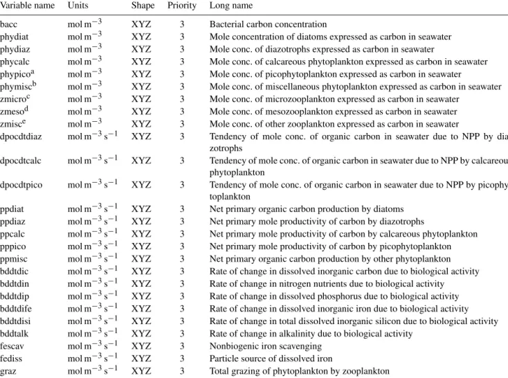
For theomip1simulation, biogeochemical tracers will be initialized generally with observational climatologies. Fields from the 2013 World Ocean Atlas (WOA2013) will be used to initialize model fields of oxygen (Garcia et al., 2014a) as well as nitrate, total dissolved inorganic phosphorus, and to-

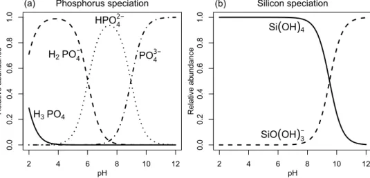
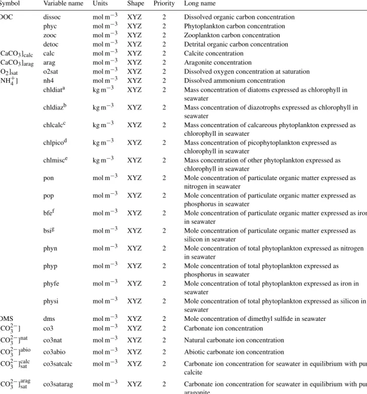
tal dissolved inorganic silicon (Garcia et al., 2014b). The latter two nutrients are often referred to simply as phosphate and silicate, but other inorganic P and Si species also contribute substantially to each total concentration (Fig. 3). In- deed it is the total dissolved concentrations (P_T and Si_T) that are both modeled and measured. OMIP will provide all these initial biogeochemical fields by merging WOA2013’s means for January, available down to 500 m (for nitrate, phosphate, and silicate), and down to 1500 m for oxygen, with its annual-mean fields below.

Model fields forA_T and preindustrialC_Twill be initialized with gridded data from version 2 of the Global Ocean Data Analysis Project (GLODAPv2) from Lauvset et al.

(2016), based on discrete measurements during WOCE and CLIVAR (Olsen et al., 2016). For greater consistency with GLODAPv1, OMIP-BGC model groups will use theCTand AT fields from GLODAPv2’s first period (1986–1999, the WOCE era).

To initialize modeled dissolved organic carbon (DOC), OMIP provides fields from the adjoint model from Schlitzer (Hansell et al., 2009). For dissolved iron (Fe), OMIP simulations will not be initialized from observations because a full-depth, global 3-D data climatology is unavailable due to lack of data coverage, particularly in the deep ocean. Hence for initial Fe fields, OMIP provides the median model result from the Iron Model Intercomparison Project (FeMIP, Tagliabue et al., 2016). Yet that initialization field may not be well suited for all Fe models, which differ greatly. Although OMIP provides initialization fields for Fe and DOC, their ac- tual initialization is left to the discretion of each modeling group. In a previous comparison (Kwiatkowski et al., 2014), groups did not initialize modeled Fe with a common field or approach because the complexity of the Fe cycle differed greatly between models. Likewise, there was no common approach to initialize DOC because biogeochemical models vary greatly in the way they represent its lability. Ini- tialization of other tracers is less critical (e.g., phytoplankton biomass is restricted to the top 200 m and equilibrates rapidly, as do other biological tracers).

Theomip1simulation is relatively short and is thus man- ageable by all groups, but many of its tracers will have large drifts because model initial states will be far from their equilibrium states. These drifts complicate assessment of model performance based on model–data agreement (Séférian et al., 2016). Hence a complementary simulation, omip1-spunup, is proposed, where biogeochemical tracers are initialized instead with a near-equilibrium state. Model groups may gen- erate this spun-up initial state by any means at their disposal.

The classic approach would be to spin up the model. That could be done either online, repeating many times the same physical atmospheric forcing (CORE-II), or offline, repeat- edly cycling the physical transport fields from a circulation model forced by a single loop of the CORE-II forcing.

If the spin-up simulation is made online, groups should reset their model’s physical fields at the end of every fifth cy-

(8)

2 4 6 8 10 12

0.00.20.40.60.81.0

Phosphorus speciation

pH

Relative abundance

H3 PO4

H2 PO₄⁻

HPO₄²⁻

PO₄³⁻

2 4 6 8 10 12

0.00.20.40.60.81.0

Silicon speciation

pH

Relative abundance

SiO

(

OH

)

₃⁻

Si

(

OH

)

₄

pH

(a) (b)

Figure 3.Relative molar abundance of inorganic species of phosphorus (left) and silicon (right) as a function of pH (total scale) in seawater at a temperature of 18^◦C and salinity of 35.

cle of CORE-II forcing to their state at the beginning of the previous third cycle. Thus groups will avoid long-term drift in the model’s physical fields, and the latter will not diverge greatly from those of theocmip1simulation but be allowed to evolve freely over a period roughly equivalent to that of the transient CO2 increase (last three forcing cycles). Con- versely, biogeochemical fields should not be reset. The end of the spin-up simulation will be reached only after many repe- titions of the five consecutive forcing cycles with the online model. That final state (i.e., the physical and biogeochemical fields from the end of the final fifth cycle) will be used to initialize theocmip1-spunupsimulation. Offline spin-up simulations should be performed in a consistent fashion. That is, groups should first integrate their circulation model over two cycles of forcing and then use the physical circulation fields generated during the third forcing cycle to subsequently drive their offline biogeochemical model, typically until they reach the criteria described below.

If possible, the spin-up should be run until it reaches the biogeochemical equilibrium criteria adopted for OCMIP2.

These criteria state that the globally integrated, biotic and abiotic air–sea CO₂ fluxes (F_CO₂ and F_COabio

2 ) should each drift by less than 0.01 Pg C year⁻¹ (Najjar and Orr, 1999;

Orr et al., 1999b) and that abiotic¹⁴C_Tshould be stabilized to the point that 98 % of the ocean volume has a drift of less than 0.001 ‰ year⁻¹(Aumont et al., 1998). The latter is equivalent to a drift of about 10 years in the¹⁴C age per 1000 years of simulation. For most models, these drift criteria can be reached only after integrations of a few thou- sand model years. To reach the spun-up state with the classic approach, i.e., with the online or offline methods outlined above, we request that groups spin up their model for at least 2000 years, if at all possible. Other approaches to obtain the spun-up state, such as using tracer-acceleration techniques or fast solvers (Li and Primeau, 2008; Khatiwala,

2008; Merlis and Khatiwala, 2008), are also permissible. If used, they should also be applied until models meet the same equilibrium criteria described above.

The spin-up simulation itself should be initialized as for theomip1simulation, except for the abiotic tracers and the

13CTtracer. The abiotic initial fields ofAâbio_T andC_Tâbiowill be provided, being derived from initial fields ofT andS. Al- thoughC_Tâbiois a passive tracer carried in the model,Aâbio_T is not. The latter will be calculated from the initial 3-D salinity field as detailed below; then that calculated field will be used to computeC_Tâbiothroughout the water column assum- ing equilibrium with the preindustrial level of atmospheric CO₂ at the initial T and S conditions (using OMIP’s carbonate chemistry routines). For ¹⁴C_Tâbio, initial fields will be based on those from GLODAPv1 for natural1¹⁴C (Key et al., 2004). OMIP will provide these initial fields with miss- ing grid cells filled based on values from adjacent ocean grid points. Groups that include¹³CTinomip1-spunupshould initialize that in the precursor spin-up simulation to 0 ‰ following the approach of Jahn et al. (2015). Beware though that equilibration timescales for¹³C are longer than forCT, im- plying the need for a much longer spin-up.

2.3 Geochemical atmospheric forcing

The atmospheric concentration histories of the three inert chemical tracers (CFC-11, CFC-12, and SF6) to be used in OMIP are summarized by Bullister (2015) and shown in Fig. 1. Their atmospheric values are to be held to zero for the first three cycles of the CORE-II forcing, then increased starting on 1 January 1936 (beginning of model year 0237) according to the OMIP protocol. To save computa- tional resources, the inert chemical tracers may be activated only from 1936 onward, starting from zero concentrations in the atmosphere and ocean. The atmospheric CO₂ history used to force the OMIP models is the same as that used for

(9)

the CMIP6 historical simulation (Meinshausen et al., 2016), while carbon isotope ratios (1¹⁴C andδ¹³C) are the same as those used by C4MIP (Jones et al., 2016). These atmospheric records of CO₂and carbon isotope ratios (Fig. 2) and those for the inert chemical tracers will be available at input4mips (https://esgf-node.llnl.gov/search/input4mips). The biogeochemical tracers are to be activated at the beginning of the 310-year simulation (on 1 January 1700) but initialized dif- ferently as described above for omip1 and omip1-spunup.

The atmospheric concentration of CO₂is to be maintained at the CMIP6 preindustrial reference ofxCOâtm₂ =284.32 ppm between calendar years 1700.0 and 1850.0, after which it must increase following observations (Meinshausen et al., 2016). The increasing xCOâtm₂ will thus affect CT but not C_T^nat, which sees only the preindustrial reference level of xCOâtm₂ . The increasingxCOâtm₂ is also seen by¹³CTand the two abiotic tracers, C_Tâbio and¹⁴C_Tâbio, to be modeled only in theomip1-spunupsimulation and its spin-up, the latter of which imposes a constant preindustrialxCOâtm₂ .

2.4 Conservation equation

The time evolution equation for all passive tracers is given by

∂C

∂t =L(C)+JC, (1)

whereC is the tracer concentration; Lis the 3-D transport operator, which represents effects due to advection, diffusion, and convection; andJCis the internal source–sink term.

Conservation of volume is assumed in Eq. (1) and standard units of mol m⁻³are used for all tracers. For the inert chemical tracers (CFC-11, CFC-12, and SF₆),J_C=0. For the abiotic carbon tracers, in theomip1-spunupsimulation and its spin-up, the same term is also null for the total carbon tracer C_T

J_Cabio T

=0, (2)

but not for the total radiocarbon tracer¹⁴C^abio_T due to radioactive decay

J14C^abio_T = −λ¹⁴C_T^abio, (3) whereλis the radioactive decay constant for¹⁴C, i.e., λ=ln(2)/5700 years=1.2160×10⁻⁴years⁻¹, (4) converted to s⁻¹ using the number of seconds per year in a given model. For other biogeochemical tracersJCis non- zero and often differs between models. For¹³CT,JCincludes isotopic fractionation effects.

2.5 Air–sea gas exchange

Non-zero surface boundary conditions must also be included for all tracers that are affected by air–sea gas exchange: CFC- 11, CFC-12, SF₆, dissolved O₂, and dissolved inorganic carbon in its various modeled forms (C_T,C_T^nat,C_T^abio,¹⁴C_T^abio,

and ¹³CT). In OCMIP2, surface boundary conditions also included a virtual-flux term for some biogeochemical tracers, namely in models that had a virtual salt flux because they did not allow water transfer across the air–sea interface.

Water transfer calls for different implementations depending on the way the free surface is treated, as discussed extensively by Roullet and Madec (2000). Groups that have im- plemented virtual fluxes for active tracers (T andS) should follow the same practices to deal with virtual fluxes of passive tracers such asC_TandA_T, as detailed in the OCMIP2 design document (Najjar and Orr, 1998) and in the OCMIP2 Abiotic HOWTO (Orr et al., 1999b). In OMIP, all models should report air–sea CO2fluxes due to gas exchange (FCO₂, F_CO^nat

2 ,F_COabio

2 ,F14CO^abio₂ , andF13CO2) without virtual fluxes included. Virtual fluxes are not requested as they do not directly represent CO₂exchange between the atmosphere and ocean.

Surface boundary fluxes may be coded simply as adding source–sink terms to the surface layer, e.g.,

JA= F_A 1z1

, (5)

where for gasA,J_Ais its surface-layer source–sink term due to gas exchange (mol m⁻³s⁻¹) and F_A is its air-to-sea flux (mol m⁻²s⁻¹), while1z1is the surface-layer thickness (m).

In OMIP, we parameterize air–sea gas transfer of CFC- 11, CFC-12, SF6, O2, CO2,¹⁴CO2, and¹³CO2using the gas transfer formulation also adopted for OCMIP2 (excluding effects of bubbles):

F_A=k_w ([A]_sat− [A]), (6) where for gasA, k_w is its gas transfer velocity, [A] is its simulated surface-ocean dissolved concentration, and[A]_sat is its corresponding saturation concentration in equilibrium with the water-vapor-saturated atmosphere at a total atmospheric pressurePa. Concentrations throughout are indicated by square brackets and are in units of mol m⁻³.

For all gases that remain purely in dissolved form in seawater, gas exchange is modeled directly with Eq. (6). How- ever, forC_T, only a small part remains as dissolved gas as mentioned in Sect. 2.6. Thus the dissolved gas concentration CO^∗₂

must first be computed, each time step, from mod- eledC_TandA_T, and then the gas exchange is computed with Eq. (6). For example, for the two abiotic tracers (inomip1- spunup),

F_COabio 2

=kw CO^∗₂

sat− CO^∗₂

(7) and

F14CO^abio₂ =k_w h

14CO^∗₂i

sat

−h

14CO^∗₂i

. (8)

For ¹³C, isotopic fractionation associated with gas exchange must be included in the flux calculation. We recom-

(10)

mend using the formulation of Zhang et al. (1995):

F13CO2 =kw αkαaq−g 13Ratm CO^∗₂

sat− ₁₃

CO^∗₂ α_C_T_−g

! , (9) whereα_kis the kinetic fractionation factor,α_aq−gis the fractionation factor for gas dissolution,α_C_T_−gis the equilibrium fractionation factor between dissolved inorganic carbon and gaseous CO2, and¹³Ratmis the¹³C/¹²C ratio in atmospheric CO2. Following Zhang et al. (1995), α_C_T−g depends on T and the fraction of carbonate inCT, namelyfCO3:

α_C_T_−g=0.0144TcfCO3−0.107Tc+10.53

1000 +1, (10)

where T_c is temperature in units of ^◦C, while division by 1000 and addition of 1 converts the fractionation factor from in units of ‰ intoα. Theα_aq−gterm depends on temperature following

α_aq−g=0.0049Tc−1.31

1000 +1. (11)

Conversely no temperature dependence was found for αk. Hence we recommend that OMIP modelers use a constant value for αkof 0.99912 (k of−0.88 ‰), the average from the Zhang et al. (1995) measurements at 5 and 21^◦C.

2.5.1 Gas transfer velocity

OMIP modelers should use the instantaneous gas transfer velocity kw parameterization from Wanninkhof (1992), a quadratic function of the 10 m wind speedu

k_w=a Sc

660 −1/2

u²(1−f_i), (12) to which we have added limitation from sea-ice cover following OCMIP2. Herea is a constant,Scis the Schmidt number, andf_i is the sea-ice fractional coverage of each grid cell (varying from 0 to 1). Normally, the constantais adjusted so that wind speeds used to force the model are consistent with the observed global inventory of bomb¹⁴C, e.g., as done in previous phases of OCMIP (Orr et al., 2001; Najjar et al., 2007). Here though, we choose to use one value of a for all simulations, independent of whether models are used in forced (OMIP) or coupled mode, namely the CMIP6 DECK (Diagnostic, Evaluation and Characterization of Klima) and historical simulations. For a in OMIP, we rely on the re- assessment from Wanninkhof (2014), who used improved estimates of the global-ocean bomb-¹⁴C inventory along with CCMP (Cross Calibrated Multi-Platform) wind fields in an inverse approach with the Modular Ocean Model (Sweeney et al., 2007) to derive a best value of

a=0.251 cm h⁻¹

(m s⁻¹)², (13)

which will givekw in cm h⁻¹if winds speeds are in m s⁻¹. For model simulations where tracers are carried in mol m⁻³, kwshould be in units of m s⁻¹; thus,ashould be set equal to 6.97×10⁻⁷m s⁻¹. The same value ofa should be adopted for the forced OMIP simulations and for ESM simulations made under CMIP6.

2.5.2 Schmidt number

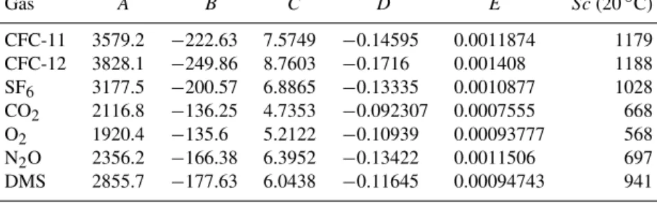
Besides a, the Schmidt numberScis also needed to compute the gas transfer velocity (Eq. 12). The Schmidt number is the ratio of the kinematic viscosity of waterν to the diffusion coefficient of the gas D (Sc=ν/D). The coefficients for the fourth-order polynomial fit ofScto in situ temperature over the temperature range of−2 to 40^◦C (Wan- ninkhof, 2014) are provided in Table 1 for each gas to be modeled in OMIP and CMIP6. Fortran 95 routines using the same formula and coefficients for all gases modeled in OMIP are available for download via thegasxmodule of themocsy package (Sect. 2.6).

2.5.3 Atmospheric saturation concentration

The surface gas concentration in equilibrium with the atmosphere (saturation concentration) is

[A]_sat =K₀f_A=K₀C_fp_A (14)

=K0Cf (Pa−pH2O) xA,

where for gasA,K₀is its solubility,f_A is its atmospheric fugacity,C_fis its fugacity coefficient,p_Ais its atmospheric partial pressure, andx_A is its mole fraction in dry air, while Pa is again the total atmospheric pressure (atm) andpH2O is the vapor pressure of water (also in atm) at sea surface temperature and salinity (Weiss and Price, 1980).

The combined term K0Cf (Pa−pH2O)is available at Pa=1 atm (i.e.,P_a⁰) for all modeled gases except oxygen.

We denote this combined term asφ_A⁰ (atP_a⁰); elsewhere it is known as the solubility functionF (e.g., Weiss and Price, 1980; Warner and Weiss, 1985; Bullister et al., 2002), but we do not use the latter notation here to avoid confusion with the air–sea flux (Eq. 6). For four of the gases to be modeled in OMIP, the combined solubility functionφ⁰_A has been computed using the empirical fit

ln φ⁰_A

=a₁+a₂ 100

T

+a₃ ln T

100

+a₄ T

100 2

+S

"

b1+b2

T 100

+b3

T 100

2#

, (15) whereT is the model’s in situ, absolute temperature (ITS90) and S is its salinity on the practical salinity scale (PSS- 78). Thus separate sets of coefficients are available for CO₂ (Weiss and Price, 1980, Table VI), CFC-11 and CFC-12 (Warner and Weiss, 1985, Table 5), and SF₆(Bullister et al.,

(11)

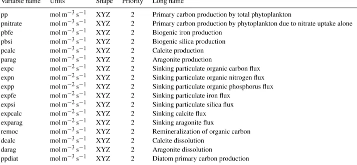
Table 1.Seawater coefficients for fit ofScto temperature^a,bfrom Wanninkhof (2014).

Gas A B C D E Sc(20^◦C)

CFC-11 3579.2 −222.63 7.5749 −0.14595 0.0011874 1179

CFC-12 3828.1 −249.86 8.7603 −0.1716 0.001408 1188

SF₆ 3177.5 −200.57 6.8865 −0.13335 0.0010877 1028 CO₂ 2116.8 −136.25 4.7353 −0.092307 0.0007555 668

O₂ 1920.4 −135.6 5.2122 −0.10939 0.00093777 568

N₂O 2356.2 −166.38 6.3952 −0.13422 0.0011506 697

DMS 2855.7 −177.63 6.0438 −0.11645 0.00094743 941

aCoefficients for fit toSc=A+BTc+CT_c²+DT_c³+ET_c⁴, whereTcis surface temperature in^◦C.

bConservative temperature should be converted to in situ temperature before using these coefficients.

Table 2.Coefficients for fit^a,b,cof solubility functionφ_A⁰ (mol L⁻¹atm⁻¹).

Gas a₁ a₂ a₃ a₄ b₁ b₂ b₃

CFC-11 −229.9261 319.6552 119.4471 −1.39165 −0.142382 0.091459 −0.0157274 CFC-12 −218.0971 298.9702 113.8049 −1.39165 −0.143566 0.091015 −0.0153924 SF₆ −80.0343 117.232 29.5817 0.0 0.0335183 −0.0373942 0.00774862 CO₂ −160.7333 215.4152 89.8920 −1.47759 0.029941 −0.027455 0.0053407 N₂O −165.8806 222.8743 92.0792 −1.48425 −0.056235 0.031619 −0.0048472

aFit to Eq. (15), whereTis in situ, absolute temperature (K) andSis salinity (practical salinity scale).^bFor units of mol m⁻³atm⁻¹, coefficients should be multiplied by 1000.^cThe units refer to atm of each gas, not atm of air.^dWhen using these coefficients, conservative temperature should be converted to in situ temperature (K) and absolute salinity should be converted to practical salinity.

2002, Table 3), the values of which are summarized here in Table 2. For O₂, it is notφ_A⁰that is available, but rather [O₂]⁰_sat (Garcia and Gordon, 1992), as detailed below.

Both the solubility functionφ_A⁰ and the saturation concentration [A]⁰_sat can be used at any atmospheric pressure Pa, with errors of less than 0.1 %, by approximating Eq. (14) as [A]_sat= Pa

P_a⁰ φ_A⁰ x_A= Pa

P_a⁰ [A]⁰

sat, (16)

whereP_a⁰is the reference atmospheric pressure (1 atm). Vari- ations in surface atmospheric pressure must not be neglected in OMIP because they alter the regional distribution of[A]_sat. For example, the average surface atmospheric pressure between 60 and 30^◦S is 3 % lower than the global mean, thus reducing surface-ocean pCO₂ by 10 µatm and [O₂]_sat by 10 µmol kg⁻¹. The atmospheric pressure fields used to compute gas saturations should also be consistent with the other physical forcing. Thus for the OMIP forced simulations, modelers will use surface atmospheric pressure from CORE II, converted to atm.

For the two abiotic carbon tracers, abbreviating K⁰= K0 Cf, we can write their surface saturation concentrations (Eq. 14) as

CO^∗₂abio

sat =K⁰ (Pa−pH2O) xCO₂ (17)

and

h14CO^∗₂iabio sat

=

CO^∗₂abio sat

14r_atm⁰ . (18)

Here¹⁴r_atm⁰ represents the normalized atmospheric ratio of

14C/C, i.e.,

14r_atm⁰ =

14ratm 14rstd

=

1+1¹⁴Catm

1000

, (19)

where ¹⁴ratm is the atmospheric ratio of ¹⁴C/C, ¹⁴rstd is the analogous ratio for the standard (1.170×10⁻¹²; see Appendix A), and 1¹⁴C_atm is the atmospheric 1¹⁴C, the fractionation-corrected ratio of¹⁴C/C relative to a standard reference given in permil (see below). We define¹⁴r_atm⁰ and use it in Eq. (18) to be able to compare¹⁴C_Tâbio andC_Tâbio directly, potentially simplifying code verification and testing. With the above model formulation for the OMIP equilibrium run (where xCOâtm₂ =284.32 ppm and 1¹⁴Câtm= 0 ‰), bothC_Tâbioand¹⁴C_Tâbiohave identical units. Short tests with the same initialization for both tracers can thus verify consistency. Differences in the spin-up simulation will stem only from different initializations and radioactive decay. Dif- ferences will grow further during the anthropogenic perturbation (inomip1-spunup, i.e., after spin-up) because of the sharp contrast between the shape of the atmospheric histories ofxCO₂and1¹⁴C_atm.