Variability and trends in Southern Ocean eddy activity in 1/12° ocean model simulations
Lavinia Patara1, Claus W. Böning1, and Arne Biastoch1
1GEOMAR Helmholtz Centre for Ocean Research Kiel, Kiel, Germany
Abstract
The response of eddy kinetic energy (EKE) to the strengthening of Southern Hemisphere winds occurring since the 1950s is investigated with a global ocean model having a resolution of 1/12° in the Antarctic Circumpolar Current domain. The simulations expose regional differences in the relative importance of stochastic and wind-related contributions to interannual EKE changes. In the Pacific and Indian sectors the model captures the EKE variability observed since 1993 and confirms previous hypotheses of a lagged response to regional wind stress anomalies. Here the multidecadal trend in wind stress is reflected in an increase in EKE typically exceeding 5 cm2s 2decade 1. In the western Atlantic, EKE variability is mostly stochastic, is weakly correlated with windfluctuations, and its multidecadal trends are close to zero. The nonuniform distribution of wind-related changes in the eddy activity could affect the regional patterns of ocean circulation and biogeochemical responses to future climate change.1. Introduction
Driven by vigorous midlatitude westerly winds, the Antarctic Circumpolar Current (ACC) is the dominant fea- ture of the Southern Hemisphere circulation and one of the most eddy-rich regions in the global ocean. The ACC is a key region for the air-sea exchanges of heat, fresh water, and atmospheric trace gases [Rintoul and Naveira Garabato, 2013], and its future evolution as a sink of carbon is one of the largest uncertainties in pro- jections of future climate change [Le Quére et al., 2007;Toggweiler and Russell, 2008;Landschützer et al., 2015].
Observations indicate that the ACC transport and stratification remained relatively stable in the past decades [Böning et al., 2008;Meredith et al., 2011;Hogg et al., 2015], despite a concomitant intensification of westerly winds in conjunction with positive phases of the Southern Annular Mode [Marshall,2003]. According to the eddy saturationandeddy compensationhypotheses, the recent trends in wind forcing should have become primarily manifested in the energy of the ocean mesoscale eddyfield—through the release of potential energy via baroclinic instability—with little change in the meanflow strength of the large-scale circulation [Straub, 1993;Hallberg and Gnanadesikan, 2006;Farneti et al., 2010;Viebahn and Eden, 2010;Munday et al., 2013;Morrison and Hogg, 2013]. However, significant uncertainty still remains regarding the role of mesoscale eddies in affecting the sensitivity of the Southern Ocean circulation to climate change.
Ocean mesoscale eddies themselves exhibit a complicated relationship to atmospheric forcing. Satellite alti- metry and some ocean models support the notion of a 1–3 year lagged response of eddy kinetic energy (EKE) to wind stress anomalies [Meredith and Hogg, 2006;Screen et al., 2009;Morrow et al., 2010;Langlais et al., 2015], while other modelsfind that a 1–3 year lag is indistinguishable from other possibilities [Wilson et al., 2014]. Satellite altimetry additionally reveals a positive trend in the Southern Ocean EKE since the early 1990s concomitant with the continuing increase in westerly winds [Hogg et al., 2015]. This deterministic view of wind-eddy interaction seems, however, at odds with recent studies showing that a large proportion of the interannual to decadal ocean variability in the ACC region is of an intrinsic or stochastic nature rather than of a forced origin [Penduff et al., 2010;O’Kane et al., 2013;Wilson et al., 2014;Sérazin et al., 2015]. Low-frequency stochastic variability is associated with the dynamics of eddy-meanflow interaction [Hogg and Blundell, 2006;
Le Bars et al., 2016] and is typically highest within the main unstable currents [Sérazin et al., 2015].
An estimate of Southern Ocean EKE changes in the past several decades is not available from the satellite altimeter record, which exists only since 1993. Inferences from global ocean models at an eddying resolution are hampered by spurious trends partly due to the high computational expenses that prevent fully adjusted simulations [Tréguier et al., 2010]. In this study a novel set of simulations is performed using a global ocean general circulation model with realistic topography and forcing, achieving a 1/12° horizontal resolution in the ACC regime through a nesting technique. A hindcast simulation from 1948 to 2007, in conjunction with
PUBLICATIONS
Geophysical Research Letters
RESEARCH LETTER
10.1002/2016GL069026
Key Points:
•A high-resolution ocean model captures the temporal variability of observed eddy kinetic energy over several regions of the Southern Ocean
•Eddy kinetic energy (EKE) increased by 17% since the 1950s, but spatial patterns are nonuniform
•Stochastic variability of EKE masks wind-driven changes in certain regions of the Southern Ocean
Supporting Information:
•Supporting Information S1
•Movie S1
•Movie S2
Correspondence to:
L. Patara, lpatara@geomar.de
Citation:
Patara, L., C. W. Böning, and A. Biastoch (2016), Variability and trends in Southern Ocean eddy activity in 1/12°
ocean model simulations,Geophys. Res.
Lett.,43, 4517–4523, doi:10.1002/
2016GL069026.
Received 30 NOV 2015 Accepted 27 APR 2016
Accepted article online 29 APR 2016 Published online 14 MAY 2016
©2016. American Geophysical Union.
All Rights Reserved.
a simulation using a repeated“normal-year”forcing, is assessed against altimeter data and previous studies and used to investigate (1) the relative contribution of stochastic processes in affecting EKE variations in dif- ferent sectors of the ACC and (2) the regional response patterns of EKE to the variability and trends of the atmospheric forcing in the period 1958 to 2007.
2. Methods
A set of simulations was performed with the NEMO-LIM2 ocean-sea ice model [Madec, 2008], where the AGRIF“two-way”nesting technique [Debreu et al., 2008] was used to enhance the horizontal resolution in the ACC regime, except for a small discontinuity between 69.5°E and 76.5°E (whose effect on the propagation of mesoscale eddies was found to be negligible as described in Text S1 in the supporting information).
Specifically, a 1/12° model was embedded between 30°S and 68°S within a 1/4° global configuration of NEMO (ORCA025) developed within the DRAKKAR collaboration [DRAKKAR Group, 2007]. A grid spacing of
~6 km is thereby achieved at 50°S, compared with a Rossby radius of ~18 km at 50°S [Chelton et al., 2011].
Eddy parameterizations are not used in either model component. This configuration, hereafter named ORION12 (Figure 1 and Movie S1), was used to perform two experiments. In a hindcast experiment (hereafter HIND), ORION12 was forced with bulk formulas using the CORE.v2 atmospheric data set [Large and Yeager, 2009] over the period 1948–2007. A companion climatological experiment (hereafter CLIM) was integrated under the CORE.v2 normal-year forcing, i.e., a repeated annual cycle retaining synoptic variability. The CLIM experiment was initialized with temperature and salinity from the World Ocean Atlas [Levitus et al., 1998] and integrated for 90 years. The HIND experiment was initialized from the 31st year of the CLIM experi- ment and integrated between 1948 and 2007. To achieve a better representation of Antarctic Bottom Water, relaxation to temperature and salinityfields given by the World Ocean Atlas [Levitus et al., 1998] was applied in areas of recently formed Antarctic Bottom Water (see Text S2 in the supporting information).
The simulated sea surface height (SSH) variance (a measure of surface geostrophic eddy variability) is com- pared with that computed from absolute dynamic topography obtained from the Archiving, Validation, and Interpretation of Satellite Oceanographic data (AVISO) product available since 1993. SSH variance in Figure 1.Variance of 5 day means of sea surface height (SSH). (a) SSH variance in ORION12 averaged between 1993 and 2007; contours show the 1/12° nested domain, (b and c) zonal averages of SSH variance in the (Figure 1b) east Indian sector (76.5°E–180°E) and in the (Figure 1c) Pacific sector (180°E–76°W) for the AVISO satellite product (red line), ORCA025 (grey line), and ORION12 (blue line), (d) meridional average (30°S–70°S) of SSH variance in the Indian sector for the AVISO satellite product (red line), ORCA025 (grey line), ORION12 nested model (thick blue line), and ORION12 host model (dashed blue line).
ORION12 is close to the satellite estimates in terms of magnitude and spatial structure (Figures 1b–1d). As a comparison, a companion stand-alone ORCA025 simulation also captures the main features of the observed SSH variance, albeit with lower values.
The analysis focuses on the interannual and multidecadal variations of EKE at 100 m depth, where direct wind-driven ocean velocities should be negligible (a justification of this choice is found in Text S3 in the sup- porting information). EKE was computed based on 5 day means of the model output, using an averaging per- iod of 1 year. To facilitate the analysis of EKE over the ACC domain and associated EKE hot spots, an averaging mask based on ACC streamlines and mean EKE values was applied (Figure 2a) and used to perform regional averages over different ACC sectors. For the analysis of interannual EKE variability, the CLIM and HIND experi- ments were detrended at each grid point with their own linearfit. The percentage of the total year-to-year variance of stochastic nature was computed byfirst spatially averaging the detrended annually averaged EKE time series over the sectors of the ACC (Figure 2a) and subsequently by computing the intrinsic-to-total ratio of EKE variance (hereafter I/T ratio) asσ2CLIM=σ2HIND100 [Penduff et al., 2010], whereσ2CLIMandσ2HINDare the EKE variances of the CLIM and HIND experiments.
Accounting for residual spurious trends unrelated to the atmospheric forcing [Tréguier et al., 2010] appears critical for assessing the long-term trends in HIND (Figures S1b–S1d). For the analysis of EKE multidecadal trends, the HIND experiment was therefore detrended at each grid point with the linearfit of the CLIM experi- ment, in the reasonable assumption that the two experiments have a similar rate of internal adjustment lead- ing to similar model spurious drifts. In the following, the interannual variability and the multidecadal trends of HIND are analyzed between 1958 and 2007, with thefirst 10 years of the HIND experiment treated as spin-up.
3. Results
Along the path of the ACC, simulated mean EKE has values typically ranging between 50 and 500 cm2s 2, with local maxima up to 1000 cm2s 2downstream of large topographic barriers (Figure 2a). This is consistent with observational estimates based on satellite and drifter data [Trani et al., 2011;Frenger et al., 2015]. The interannual variability of EKE over the satellite era is also well captured. Averaged over the whole ACC domain, the model exhibits lower EKE values in the mid-1990s and a peak in 2000–2002, in agreement with the AVISO satellite product (Figure 3a). A diversified picture emerges, however, when analyzing the temporal evolution of EKE over different sectors of the ACC (Figures 3b–3f). In the lee of Kerguelen Plateau (Figure 3b), south of Australia (Figure 3c), and in the central Pacific (Figure 3d) the match between model and satellite is good (with correlation coefficients of 0.61, 0.53, and 0.60, respectively, all statistically significant at 95%), Figure 2.EKE at 100 m depth in the ACC domain. (a) Colors: EKE in HIND (1958–2007 average), contours: 5 Sv and 110 Sv contours of the barotropic stream function, boxes: sectors used for spatial averages, (b) intrinsic-to-total ratio of EKE variance on interannual time scales over ACC sectors, (c) EKE linear trends in HIND between 1958 and 2007 averaged over sectors, where only trends that are statistically significant at 95% are shown; sector numbers are superimposed in black.
The ACC domain is defined using the following criteria: (1) the ocean barotropic stream function is included between 5 Sv and 110 Sv and/or (2) EKE is higher than 45 cm2s 2, with both quantities spatially smoothed prior this computation, and (3) regions corresponding to the Malvinas Current and the Agulhas Return Current are manually removed.
Geophysical Research Letters
10.1002/2016GL069026whereas in the vicinity of Drake Passage (Figure 3e) and in the western Atlantic (Figure 3f), the model and the satellite time series are totally uncorrelated on interannual time scales.
This result can be rationalized by considering, for each sector, the percentage of EKE variance which is of a sto- chastic nature rather than of a forced origin, i.e., by analyzing the intrinsic-to-total ratio of EKE variance (Figure 2b). The I/T ratio provides afirst estimate of the regions in which wind-driven responses of EKE are more likely to be masked by stochastic variability. It is found that in general, the sectors where the match between model and satellite is best are also characterized by a comparatively lower I/T ratio. On the other hand, in sectors where the match with the satellite product is poor, the I/T ratio exceeds 75%. As discussed in section 4, the high I/T ratio in the Atlantic sector, which is in agreement with previous studies [Sérazin et al., 2015], is possibly related to the combination of distinct topographic properties and low wind stress forcing. The substantial con- tribution of stochastic processes to the total EKE variance at Drake Passage and in the western Atlantic helps explaining the mismatch between simulated and observed EKE in those regions (Figures 3e and 3f).
The relation between interannually varying winds and EKE is investigated by computing correlation coefficients between linearly detrended and regionally averaged time series of total wind stress and EKE Figure 3.Time series of simulated EKE at 100 m depth and of satellite-observed surface EKE. Red lines: CLIM (years 41 to 89), blue lines: HIND (years 1958 to 2007), and black lines: AVISO satellite product (years 1993 to 2007). Spatial averages are performed over (a) the whole ACC domain and over (b–f) sectors of the ACC (corresponding sector numbers are shown in Figure 2c); correlation coefficients between simulated and observed EKE over the period 1993–2007 are shown at the bottom right of each panel (an asterisk indicates a 95% statistically significant correlation). EKE in HIND was detrended with the linearfit of CLIM (dashed red line). The time axis refers to the HIND experiment. The leftyaxis refers to both CLIM and HIND; notice the differentyaxis for simulated and observed EKE.
(Figure 4a). Interestingly, wefind that correlations of EKE with regionally averaged wind stress are overall higher than with circumpolar wind stress or with the Southern Annular Mode index (Figure S2a), pointing to the importance of regional wind stress forcing in determining an EKE response. Consistent with previous hypotheses of wind-EKE interaction [Meredith and Hogg, 2006], an EKE increase after a wind peak often occurs with a delay ranging between 0 and 3 years depending on the ACC sector (Figure S2b). Maximum correlation coefficients over this time horizon (Figure 4a) are statistically significant at 95% in about half of the analyzed sectors, whereas at Drake Passage and in the western Atlantic correlations are at the lowest end of spectrum.
Thus, despite the importance of stochastic processes which tend to mask the wind-EKE relationship, a deter- ministic response of EKE to wind stressfluctuations can at least be identified in some regions of the ACC.
Having assessed the capability of the model in reproducing the observed EKE temporal evolution over sev- eral sectors of the ACC as well as the proposed linkage to interannual wind stressfluctuations [Meredith and Hogg, 2006], the multidecadal trends of EKE since 1958 are analyzed next. Between 1958 and 2007, an increase of EKE of 5 cm2s 2decade 1(i.e., an 17% increase) is simulated over the whole ACC (Figure 3a), con- comitant with a 26% increase in wind stress. The multidecadal changes in EKE are, however, not distributed uniformly along the path of the ACC (Figure 2c). Over large parts of the ACC, EKE multidecadal trends are sta- tistically significant and typically exceed 5 cm2s 2decade 1whereas at Drake Passage and in the western Atlantic EKE changes are close to zero. This inhomogeneous pattern of change is analogous to that found in satellite estimates since 1993 [Hogg et al., 2015].
We note that concomitant to these multidecadal changes in wind stress and EKE, the ACC volume transport and the residual meridional overturning circulation (MOC) in density space exhibit an increase of 9% and 44%, respectively (both statistically significant at 95%, see also Figures S1c and S1d). These values are com- parable to“eddy-permitting”ocean models under realistic forcing [Farneti et al., 2015] and somewhat higher (in the case of the MOC) than idealized modeling studies at a similar resolution [Morrison and Hogg, 2013], suggesting that the ACC simulated in this 1/12° model is not in a completely eddy-saturated state.
4. Summary and Discussion
The variability and trends of EKE in the Southern Ocean were investigated in multidecadal simulations with a novel global ocean model configuration having 1/12° resolution in the ACC domain and realistic topography.
The model captures the variability and trends of the satellite-derived EKE over several sectors of the ACC and overall confirms previous hypotheses of a lagged EKE response to wind stress anomalies [Meredith and Hogg, 2006] despite a substantial contribution of stochastic processes to the EKE variance. It is found that the depen- dence of EKE on wind changes is not uniformly distributed along the ACC. Over large parts of the Pacific and Indian sectors, EKE responds to wind changes, its variability matches that inferred from satellite altimetry, and a statistically significant multidecadal increase exceeding 20% since 1958 is found. On the other hand, close to Drake Passage and in the western Atlantic EKE variability is mostly stochastic, its correlation with interannual wind stressfluctuations is low, and EKE multidecadal trends are close to zero.
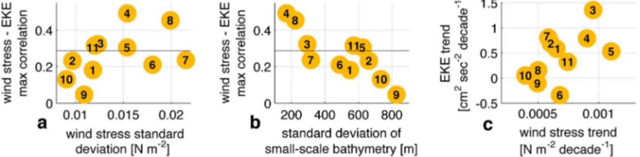
Figure 4.Scatter plots of (a) EKE-wind stress maximum correlations against wind stress standard deviation in ACC sectors (corresponding numbers in Figure 2c); the correlation value shown is the maximum in the temporal domain of 0 to 3 years lagging the wind stress; the dashed line indicates the 95% confidence level, (b) EKE- wind stress maximum correlations against the standard deviation of small-scale bathymetry in ACC sectors; the small-scale bathymetry was obtained by removing a smoothed bathymetry interpolated on a 4° grid from the original bathymetry and thus contains horizontal scales<400 km, (c) EKE multidecadal trend against total wind stress multidecadal trend in ACC sectors.
Geophysical Research Letters
10.1002/2016GL069026considered to crucially depend on the existence of topography [Hogg and Blundell, 2006;Meredith and Hogg, 2006], our model results indicate that smaller-scale topographic roughness may have the opposite effect (Figure 4b). This is possibly related to the fact that topographic roughness dissipates mesoscale eddies more effectively than a smoother ocean bottom, as found in previous studies across a range of ocean model resolu- tions and complexity [e.g.,Böning, 1989;Nikurashin et al., 2013], a behavior which might possibly interfere with the positive topographic feedback proposed byMeredith and Hogg[2006].
Since the strengthening of westerly winds is projected to continue under rising greenhouse gas emissions [Gillett and Fyfe, 2013], a concomitant increase in mesoscale eddy activity could have a global climatic impact.
It is hypothesized that mesoscale eddies might mitigate the projected reduction of the Southern Ocean car- bon sink in response to increasing westerly winds [Le Quére et al., 2007;Dufour et al., 2013;Abernathey and Ferreira, 2015]. Mesoscale eddies have also been shown to affect the properties of mode waters forming on the equatorward side of the ACC [Herraiz-Borreguero and Rintoul, 2010] as well as the transport of heat, salt, and biogeochemical tracers poleward across the ACC [Ansorge et al., 2014;Dufour et al., 2015]. A local increase in mesoscale activity could thus impact environmentally relevant properties such as water mass for- mation, the sea ice edge location, marine productivity, and marine biota. This study points to a nonuniform distribution of wind-related changes in the Southern Ocean eddy activity. Thisfinding needs to be accounted for when assessing the implications of trends in eddy-inducedfluxes on the sequestration of heat, CO2, and biogeochemical tracers in the Southern Ocean.
References
Abernathey, R., and D. Ferreira (2015), Southern Ocean isopycnal mixing and ventilation changes driven by winds,Geophys. Res. Lett.,23, 10,357–10,365, doi:10.1002/2015GL066238.
Ansorge, I., J. Jackson, K. Reid, J. Durgadoo, S. Swart, and S. Eberenz (2014), Evidence of a southward eddy corridor in the south-west Indian ocean,Deep Sea Res., Part II, doi:10.1016/j.dsr2.2014.05.012.
Böning, C. W. (1989), Influences of a rough bottom topography onflow kinematics in an eddy-resolving circulation model,J. Phys. Oceanogr., 19(1), 77–97, doi:10.1175/1520-0485(1989)019<0077:IOARBT>2.0.CO;2.
Böning, C. W., A. Dispert, M. Visbeck, S. R. Rintoul, and F. U. Schwarzkopf (2008), The response of the Antarctic Circumpolar Current to recent climate change,Nat. Geosci.,1, 864–869, doi:10.1038/ngeo362.
Chelton, D. B., M. G. Schlax, and R. M. Samelson (2011), Global observations of nonlinear mesoscale eddies,Progr. Oceanogr.,91(2), 167–216, doi:10.1016/j.pocean.2011.01.002.
Debreu, L., C. Vouland, and E. Blayo (2008), AGRIF: Adaptive grid refinement in Fortran,Comput. Geosci.,34(1), 8–13, doi:10.1016/j.cageo.2007.01.009.
DRAKKAR Group (2007), Eddy-permitting ocean circulation hindcasts of past decades,Clivar Exchange,12(3).
Dufour, C. O., J. Le Sommer, M. Gehlen, J. C. Orr, J.-M. Molines, J. Simeon, and B. Barnier (2013), Eddy compensation and controls of the enhanced sea-to-air CO2flux during positive phases of the Southern Annular Mode,Global Biogeochem. Cycles,27, 950–961, doi:10.1002/gbc.20090.
Dufour, C., et al. (2015), Role of mesoscale eddies in cross-frontal transport of heat and biogeochemical tracers in the Southern Ocean,J. Phys.
Oceanogr.,45(12), 3057–3081, doi:10.1175/JPO-D-14-0240.1.
Farneti, R., T. L. Delworth, A. J. Rosati, S. M. Griffies, and F. Zeng (2010), The role of mesoscale eddies in the rectification of the Southern Ocean response to climate change,J. Phys. Oceanogr.,40, 1539–1557, doi:10.1175/2010JPO4353.1.
Farneti, R., et al. (2015), An assessment of Antarctic Circumpolar Current and Southern Ocean Meridional Overturning Circulation during 1958–2007 in a suite of interannual CORE-II simulations,Ocean Model.,93, 84–120, doi:10.1016/j.ocemod.2015.07.009.
Frenger, I., M. Muennich, N. Gruber, and R. Knutti (2015), Southern Ocean eddy phenomenology,J. Geophys. Res. Oceans,120, 7413–7449, doi:10.1002/2015JC011047.
Gillett, N. P., and J. C. Fyfe (2013), Annular mode changes in the CMIP5 simulations,Geophys. Res. Lett.,40, 1189–1193, doi:10.1002/grl.50249.
Hallberg, R., and A. Gnanadesikan (2006), The role of eddies in determining the structure and response of the wind-driven Southern Hemisphere overturning: Results from the Modelling Eddies in the Southern Ocean (MESO) project,J. Phys. Oceanogr.,36, 2232–2251, doi:10.1175/JPO2980.1.
Herraiz-Borreguero, L., and S. R. Rintoul (2010), Subantarctic Mode Water variability influenced by mesoscale eddies south of Tasmania, J. Geophys. Res.,115, C04004, doi:10.1029/2008JC005146.
Hogg, A. M. C., and J. R. Blundell (2006), Interdecadal variability of the Southern Ocean,J. Phys. Oceanogr.,36(8), 1626–1645, doi:10.1175/JPO2934.1.
Hogg, A. M. C., M. P. Meredith, D. P. Chambers, E. P. Abrahamsen, C. W. Hughes, and A. K. Morrison (2015), Recent trends in the Southern Ocean eddyfield,J. Geophys. Res. Oceans,120, 257–267, doi:10.1002/2014JC010470.
Acknowledgments
The data for this paper are freely avail- able at thredds.geomar.de/thredds/cata- log/open_access/patara_et_al_2016_grl/
catalog.html. The integration of the experiments was performed at the North-German Supercomputing Alliance (HLRN). The study wasfinancially sup- ported by the Deutsche
Forschungsgemeinschaft (DFG) project BO 907/4-1 and by the project CP1219 of the Cluster of Excellence“The Future Ocean”funded within the framework of the Excellence Initiative by the DFG. We thank the Archiving, Validation, and Interpretation of Satellite Oceanographic data (AVISO) project for providing alti- metry data, and the NEMO and DRAKKAR teams for their technical support. We thank two anonymous reviewers for their constructive comments on a previous version of this manuscript.
Landschützer, P., et al. (2015), The reinvigoration of the Southern Ocean carbon sink,Science,349, 1221, doi:10.1126/science.aab2620.
Langlais, C. E., S. R. Rintoul, and J. D. Zika (2015), Sensitivity of Antarctic Circumpolar Current transport and eddy activity to wind patterns in the Southern Ocean,J. Phys. Oceanogr.,45(4), 1051–1067, doi:10.1175/JPO-D-14-0053.1.
Large, W. G., and S. G. Yeager (2009), The global climatology of an interannually varying air-seaflux data set,Climate Dyn.,33, 341–364, doi:10.1007/s00382-008-0441-3.
Le Bars, D., J. P. Viebahn, and H. A. Dijkstra (2016), A Southern Ocean mode of multidecadal variability,Geophys. Res. Lett.,43, 2102–2110, doi:10.1002/2016GL068177.
Le Quére, C., et al. (2007), Saturation of the Southern Ocean CO2sink due to recent climate change,Science,316(5832), 1735–1738, doi:10.1126/science.1136188.
Levitus, S., et al. (1998),World Ocean Database 1998, vol. 1, Introduction, NOAA Atlas NESDIS, 18, NOAA, Silver Spring, Md.
Madec, G. (2008), NEMO ocean engine, Note du Pole de modelisation de l’Institut Pierre-Simon Laplace 27, 217 pp.
Marshall, G. J. (2003), Trends in the Southern Annular Mode from observations and reanalyses,J. Clim.,16, 4134–4143, doi:10.1175/1520-0442 (2003)016,4134:TITSAM.2.0.CO;2.
Meredith, M. P., and A. M. Hogg (2006), Circumpolar response of Southern Ocean eddy activity to a change in the Southern Annular Mode, Geophys. Res. Lett.,33, L16608, doi:10.1029/2006GL026499.
Meredith, M. P., et al. (2011), Sustained monitoring of the Southern Ocean at Drake Passage: Past achievements and future priorities,Rev.
Geophys.,49, RG4005, doi:10.1029/2010RG000348.
Morrison, A. K., and A. M. Hogg (2013), On the relationship between Southern Ocean overturning and ACC transport,J. Phys. Oceanogr.,43, 140–148, doi:10.1175/JPO-D-12-057.1.
Morrow, R., M. L. Ward, A. M. Hogg, and S. Pasquet (2010), Eddy response to Southern Ocean climate modes,J. Geophys. Res.,115, C10030, doi:10.1029/2009JC005894.
Munday, D. R., H. L. Johnson, and D. P. Marshall (2013), Eddy saturation of equilibrated circumpolar currents,J. Phys. Oceanogr.,43(3), 507–532, doi:10.1175/JPO-D-12-095.1.
Nikurashin, M., G. K. Vallis, and A. Adcroft (2013), Routes to energy dissipation for geostrophicflows in the Southern Ocean,Nat. Geosci.,6(1), 48–51, doi:10.1038/NGEO1657.
O’Kane, T., R. Matear, M. Chamberlain, J. Risbey, B. Sloyan, and I. Horenko (2013), Decadal variability in an OGCM Southern Ocean: Intrinsic modes, forced modes and metastable states,Ocean Model.,69, 1–21, doi:10.1016/j.ocemod.2013.04.009.
Penduff, T., M. Juza, L. Brodeau, G. C. Smith, B. Barnier, J.-M. Molines, A.-M. Treguier, and G. Madec (2010), Impact of global ocean model resolution on sea-level variability with emphasis on interannual time scales,Ocean Sci.,6, 269–284, doi:10.5194/os-6-269-2010.
Rintoul, S. R., and A. C. Naveira Garabato (2013), Dynamics of the Southern Ocean, inOcean Circulation and Climate: A 21st Century Perspective, Intl. Geophys. Ser., vol. 103, edited by G. Siedler, pp. 471–492, Academic Press, Oxford.
Screen, J. A., N. P. Gillett, D. P. Stevens, G. J. Marshall, and H. K. Roscoe (2009), The role of eddies in the Southern Ocean temperature response to the Southern Annular Mode,J. Clim.,22, 806–818, doi:10.1175/2008JCLI2416.1.
Sérazin, G., T. Penduff, S. Gregorio, B. Barnier, J. M. Molines, and L. Terray (2015), Intrinsic variability of sea level from global 1/12 degrees ocean simulations: Spatiotemporal scales,J. Clim.,28(10), 4279–4292, doi:10.1175/JCLI-D-14-00554.1.
Straub, D. N. (1993), On the transport and angular momentum balance of channel models of the Antarctic Circumpolar Current,J. Phys.
Oceanogr.,23, 776–782, doi:10.1175/1520-0485(1993)023,0776:OTTAAM.2.0.CO;2.
Toggweiler, J. R., and J. Russell (2008), Ocean circulation in a warming climate,Nature,451(7176), 286–288, doi:10.1038/nature06590.
Trani, M., P. Falco, and E. Zambianchi (2011), Near-surface eddy dynamics in the Southern Ocean,Polar Res.,30, 11,203, doi:10.3402/polar.v30i0.11203.
Tréguier, A. M., J. Le Sommer, J. M. Molines, and B. de Cuevas (2010), Response of the Southern Ocean to the Southern Annular Mode:
Interannual variability and multidecadal trend,J. Phys. Oceanogr.,40, 1659–1668, doi:10.1175/2010JPO4364.1.
Viebahn, J., and C. Eden (2010), Towards the impact of eddies on the response of the Southern Ocean to climate change,Ocean Model., 34(3–4), 150–165, doi:10.1016/j.ocemod.2010.05.005.
Wilson, C., C. W. Hughes, and J. R. Blundell (2014), Forced and intrinsic variability in the response to increased wind stress of an idealized Southern Ocean,J. Geophys. Res. Oceans,120, 113–130, doi:10.1002/2014JC010315.