Supporting Information for Physical controls of Southern Ocean deep-convection variability in CMIP5 models and the Kiel Climate Model A. Reintges

Supporting Information for

Physical controls of Southern Ocean deep-convection variability in CMIP5 models and the Kiel Climate Model

A. Reintges¹, T. Martin¹, M. Latif^1,2, and W. Park¹

1 GEOMAR Helmholtz Centre for Ocean Research Kiel, Kiel, Germany

2 University of Kiel, Kiel, Germany

Corresponding author: Annika Reintges (areintges@geomar.de)

Contents of this file Discussion Tables S1 to S5 Figures S1 to S7

2 Discussion

In contrast to the findings of Latif et al. [2013] which were based on the KCM1.2a the newer versions of the KCM (KCM1.4a and KCM1.4b) simulate a much weaker impact of the

convection events on the atmosphere. The reason for that is probably the weaker intensity of the deep-convection events in the KCM1.4 versions and this might further be attributed to their weaker stratification compared to the KCM1.2 versions. This strong stratification in KCM1.2 is mainly caused by a strong vertical salinity gradient dominating the effect on density. This effect is not restricted to the convection region but prevails in the whole Atlantic sector of the Southern Ocean.

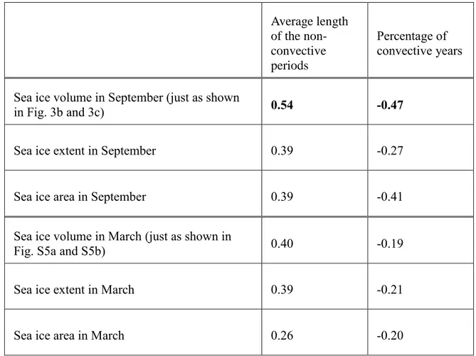
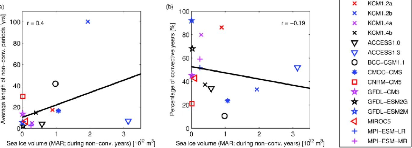
As proposed by de Lavergne et al. [2014] the sea ice cover of the preceding summer is also important for the subsequent winter deep-convection. They find that the models that do not exhibit deep-convection tend to have a large February sea ice volume. Also Heuzé et al. [2013]

find that there is an inverse relationship between the winter deep-convection intensity and the summer sea ice. They suggest in models with a large summer sea ice volume the reduced brine rejection and smaller oceanic heat loss to the atmosphere could cause the convection to be less intense. In the models analyzed here the minimum sea ice volume and extent is simulated in March. However, we do not find significant correlations of the March sea ice volume with the average length of the non-convective periods, or with the percentage of convective years (Figs.

3d and 3e).

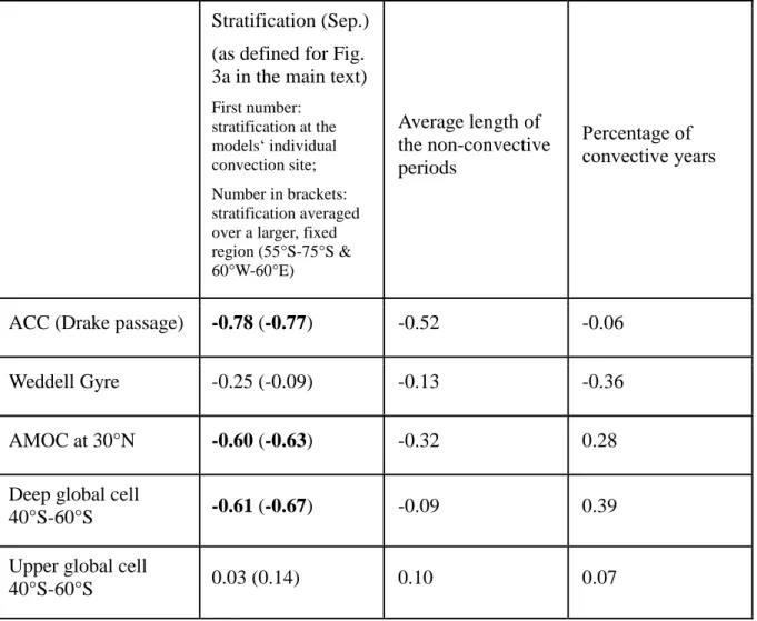
We also analyzed the relation of the two control variables (sea ice volume and stratification during non-convective years) to a number of mean circulation indices (Table S4). We find that models with a strong stratification tend to have a weaker AABW cell in the Southern Ocean, and a weaker ACC and AMOC. Clearly, the strength of the ACC is linked to the meridional density gradient between mid and high latitudes. The significant correlation with the AMOC index shows that the climate models feature the principle physics linking the meridional overturning circulation with the deep-convection in both hemispheres.

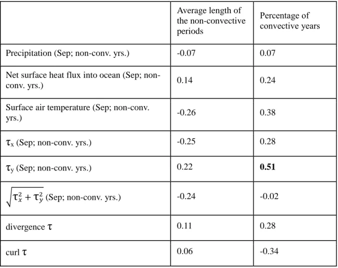
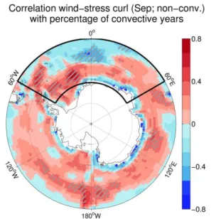
Furthermore, we tested the importance of atmospheric quantities for the measures of deep- convection variability (Table S6): No significant correlation was found between atmospheric quantities and the average lengths of non-convective periods. The percentage of convective years, however, is significantly (90% confidence level) correlated to the northward wind-stress averaged over the Atlantic sector of the Southern Ocean (for September during non-convective years: r = -0.51). A high percentage of convective years is further significantly correlated to a positive wind-stress curl over the main convection sites (Fig. S7) which promotes Ekman downwelling. Models that are predominantly in the convective regime are further characterized by a zonal gradient in sea level pressure that causes a stronger northward wind-stress in the Atlantic sector of the Southern Ocean. The cause for these relations to the deep-convection is unclear, and the question how the atmospheric mean state might affect the predominant regime of a model needs further analysis.

3

Modelling center Year provided

ACCESS1.0 CSIRO-BOM,

Australia

500

ACCESS1.3 500

BCC-CSM1.1 BCC, China 500

CMCC-CMS CMCC, Italy 500

CNRM-CM5 CNRM-CERFACS,

France 850

GFDL-CM3

NOAA-GFDL, USA 500

GFDL-ESM2G 500

GFDL-ESM2M 500

MIROC5 MIROC, Japan 670

MPI-ESM-LR

MPI-M, Germany 1000

MPI-ESM-MR 1000

Table S1. Selection of CMIP5 models; for selection criteria see main text.

4 KCM

version Resolution

atmosphere Resolution ocean

Thickness of newly formed lead ice

CO2

concentration Integration length used

Skipped spin-up time KCM1.2a

1.2

T31 (3.75°) horizontally;

19 vertical

levels 2°

horizontally;

31 vertical levels

h0 = 0.1 m

348 ppm (present-day)

2500 yrs 1000 yrs KCM1.2b

h0 = 0.6 m

2300 yrs 300 yrs KCM1.4a

1.4

T42 (2.8°) horizontally;

19 vertical levels

1800 yrs

800 yrs

KCM1.4b 286 ppm (pre-

industrial) 3700 yrs Table S2. KCM experiments.

5

Average length of the non- convective periods

Percentage of convective years

Sea ice volume in September (just as shown

in Fig. 3b and 3c) 0.54 -0.47

Sea ice extent in September 0.39 -0.27

Sea ice area in September 0.39 -0.41

Sea ice volume in March (just as shown in

Fig. S5a and S5b) 0.40 -0.19

Sea ice extent in March 0.39 -0.21

Sea ice area in March 0.26 -0.20

Table S3. Correlation coefficients analogous to Figs. 3 and S5 for different sea ice measures within the Atlantic sector of the Southern Ocean. Significant correlations are bold (90%

confidence level).

6 Stratification (Sep.) (as defined for Fig.

3a in the main text)

First number:

stratification at the models‘ individual convection site;

Number in brackets:

stratification averaged over a larger, fixed region (55°S-75°S &

60°W-60°E)

Average length of the non-convective periods

Percentage of convective years

ACC (Drake passage) -0.78 (-0.77) -0.52 -0.06

Weddell Gyre -0.25 (-0.09) -0.13 -0.36

AMOC at 30°N -0.60 (-0.63) -0.32 0.28

Deep global cell

40°S-60°S -0.61 (-0.67) -0.09 0.39

Upper global cell

40°S-60°S 0.03 (0.14) 0.10 0.07

Table S4. Correlation coefficients associated with circulation indices. The circulation indices are averaged over all months and all years. Significant correlations are bold (90% confidence level).

The ACC (Antarctic Circumpolar Current, computed at Drake Passage) and the Weddell Gyre were computed from the barotropic streamfunction. The AMOC (Atlantic Meridional Overturning Circulation) at 30°N is the maximum of the Atlantic meridional overturning streamfunction. The deep global cell is here defined as the minimum in the global meridional overturning streamfunction between 40°S and 60°S multiplied by -1; and the upper global cell is here defined as the maximum in the global meridional overturning streamfunction between 40°S and 60°S.

7

Average length of the non-convective periods

Percentage of convective years Precipitation (Sep; non-conv. yrs.) -0.07 0.07

Net surface heat flux into ocean (Sep; non-

conv. yrs.) 0.14 0.24

Surface air temperature (Sep; non-conv.

yrs.) -0.26 0.38

τ

τ

√

τ

τ

divergence

τ

curl

τ

Table S5. Correlations of convection measures with atmospheric variables.

τ

τ

8

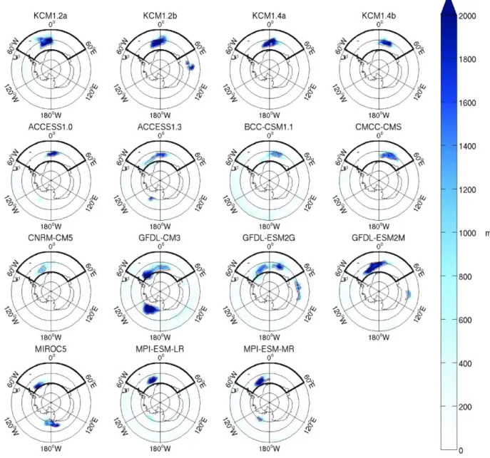
Figure S1. Standard deviation of September mean mixed layer depth. The red line encircles the main convection region of each model that is characterized by a mixed layer deeper than 3000 m in at least 5 % of all years. The Atlantic sector of the Southern Ocean is marked by the thick black contour line.

9

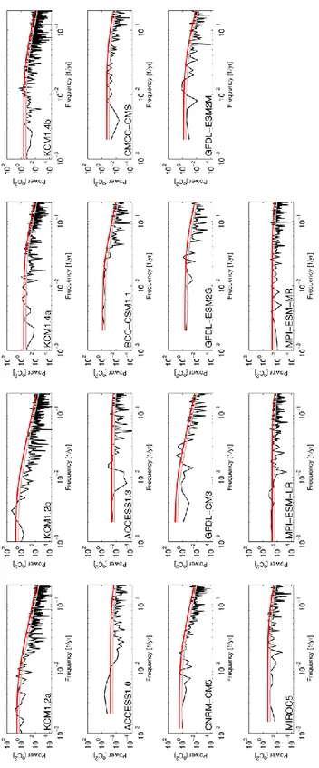
Figure S2. Power spectrum of the September SST index area-averaged over the Atlantic sector.

The grey line depicts the median spectrum of a red noise process and the red line the 95%- confidence limit.

10 Figure S3. Analogous to Figure 2 but for all models.

11

Figure S4. Profiles of all 15 models averaged over the main convection region in the Atlantic sector of the Southern Ocean and only over non-convective years of the potential temperature (left panel), the salinity (middle panel), and the potential density (right panel). The 300 m depth level is marked by a grey horizontal line.

12

Figure S5. The role of the summer sea ice volume. (a) Analogous to (Fig. 3b) but with the sea ice volume from March instead of September. (b) Analogous to (Fig. 3c) but with the sea ice volume from March instead of September.

13

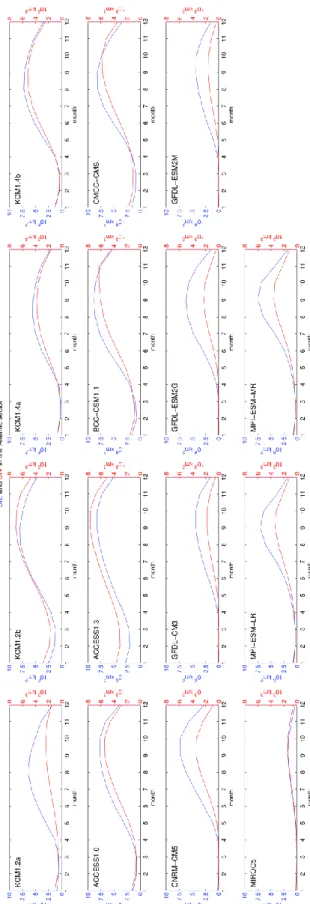
Figure S6. Seasonal cycle of the sea ice extent (blue) and the sea ice volume (red) within the Atlantic sector of the Southern Ocean.

14

Figure S7. Correlations of atmospheric mean states (for September in non-convective years) with the percentage of convective years. The atmospheric mean states are represented by the northward wind-stress (upper left panel), the wind-stress curl (upper right panel), the sea level pressure (lower left panel), and the surface air temperature (lower right panel). Significance at 90% is marked by the hatching