Evaluation of global ocean–sea-ice model simulations based on the experimental protocols of the Ocean Model

(1)

Geosci. Model Dev., 13, 3643–3708, 2020 https://doi.org/10.5194/gmd-13-3643-2020

Evaluation of global ocean–sea-ice model simulations based on the experimental protocols of the Ocean Model

Intercomparison Project phase 2 (OMIP-2)

Hiroyuki Tsujino¹, L. Shogo Urakawa¹, Stephen M. Griffies^2,3, Gokhan Danabasoglu⁴, Alistair J. Adcroft^3,2, Arthur E. Amaral⁵, Thomas Arsouze⁵, Mats Bentsen⁶, Raffaele Bernardello⁵, Claus W. Böning⁷, Alexandra Bozec⁸, Eric P. Chassignet⁸, Sergey Danilov⁹, Raphael Dussin², Eleftheria Exarchou⁵, Pier Giuseppe Fogli¹⁰,

Baylor Fox-Kemper¹¹, Chuncheng Guo⁶, Mehmet Ilicak^12,6, Doroteaciro Iovino¹⁰, Who M. Kim⁴, Nikolay Koldunov^13,9, Vladimir Lapin⁵, Yiwen Li^14,15, Pengfei Lin^14,15, Keith Lindsay⁴, Hailong Liu^14,15,

Matthew C. Long⁴, Yoshiki Komuro¹⁶, Simon J. Marsland¹⁷, Simona Masina¹⁰, Aleksi Nummelin⁶, Jan Klaus Rieck⁷, Yohan Ruprich-Robert⁵, Markus Scheinert⁷, Valentina Sicardi⁵, Dmitry Sidorenko⁹, Tatsuo Suzuki¹⁶,

Hiroaki Tatebe¹⁶, Qiang Wang⁹, Stephen G. Yeager⁴, and Zipeng Yu^14,15

1JMA Meteorological Research Institute (MRI), Tsukuba, Ibaraki, Japan

2NOAA Geophysical Fluid Dynamics Laboratory (GFDL), Princeton, NJ, USA

3Princeton University Atmospheric and Oceanic Sciences Program, Princeton, NJ, USA

4National Center for Atmospheric Research (NCAR), Boulder, CO, USA

5Barcelona Supercomputing Center, Barcelona, Spain

6NORCE Norwegian Research Centre, Bjerknes Centre for Climate Research, Bergen, Norway

7GEOMAR Helmholtz Centre for Ocean Research, Kiel, Germany

8Center for Ocean-Atmospheric Prediction Studies (COAPS), Florida State University, Tallahassee, FL, USA

9Alfred-Wegener-Institut Helmholtz-Zentrum für Polar- und Meeresforschung (AWI), Bremerhaven, Germany

10Ocean Modeling and Data Assimilation Division, Centro Euro-Mediterraneo sui Cambiamenti Climatici (CMCC), Bologna, Italy

11Department of Earth, Environmental, and Planetary Sciences, Brown University, Providence, RI, USA

12Eurasia Institute of Earth Sciences, Istanbul Technical University, Istanbul, Turkey

13MARUM-Center for Marine Environmental Sciences, Bremen, Germany

14LASG, Institute of Atmospheric Physics, Chinese Academy of Sciences, Beijing, China

15College of Earth and Planetary Sciences, University of Chinese Academy of Sciences, Beijing, China

16Japan Agency for Marine-Earth Science and Technology (JAMSTEC), Yokohama, Japan

17CSIRO Oceans and Atmosphere, Aspendale, Australia Correspondence:Hiroyuki Tsujino (htsujino@mri-jma.go.jp) Received: 24 December 2019 – Discussion started: 29 January 2020

Revised: 12 June 2020 – Accepted: 4 July 2020 – Published: 21 August 2020

Abstract. We present a new framework for global ocean–

sea-ice model simulations based on phase 2 of the Ocean Model Intercomparison Project (OMIP-2), making use of the surface dataset based on the Japanese 55-year atmospheric reanalysis for driving ocean–sea-ice models (JRA55-do). We motivate the use of OMIP-2 over the framework for the first phase of OMIP (OMIP-1), previously referred to as the Co-

ordinated Ocean–ice Reference Experiments (COREs), via the evaluation of OMIP-1 and OMIP-2 simulations from 11 state-of-the-science global ocean–sea-ice models. In the present evaluation, multi-model ensemble means and spreads are calculated separately for the OMIP-1 and OMIP-2 simulations and overall performance is assessed considering metrics commonly used by ocean modelers. Both OMIP-1 and

(2)

3644 H. Tsujino et al.: Evaluation of global ocean–sea-ice model simulations OMIP-2 multi-model ensemble ranges capture observations

in more than 80 % of the time and region for most metrics, with the multi-model ensemble spread greatly exceeding the difference between the means of the two datasets. Many features, including some climatologically relevant ocean circulation indices, are very similar between OMIP-1 and OMIP- 2 simulations, and yet we could also identify key qualita- tive improvements in transitioning from OMIP-1 to OMIP- 2. For example, the sea surface temperatures of the OMIP- 2 simulations reproduce the observed global warming during the 1980s and 1990s, as well as the warming slow- down in the 2000s and the more recent accelerated warming, which were absent in OMIP-1, noting that the last feature is part of the design of OMIP-2 because OMIP-1 forcing stopped in 2009. A negative bias in the sea-ice concentration in summer of both hemispheres in OMIP-1 is significantly reduced in OMIP-2. The overall reproducibility of both seasonal and interannual variations in sea surface temperature and sea surface height (dynamic sea level) is improved in OMIP-2. These improvements represent a new ca- pability of the OMIP-2 framework for evaluating process- level responses using simulation results. Regarding the sensitivity of individual models to the change in forcing, the models show well-ordered responses for the metrics that are directly forced, while they show less organized responses for those that require complex model adjustments. Many of the remaining common model biases may be attributed either to errors in representing important processes in ocean–sea-ice models, some of which are expected to be reduced by using finer horizontal and/or vertical resolutions, or to shared biases and limitations in the atmospheric forcing. In particular, further efforts are warranted to resolve remaining issues in OMIP-2 such as the warm bias in the upper layer, the mismatch between the observed and simulated variability of heat content and thermosteric sea level before 1990s, and the erroneous representation of deep and bottom water forma- tions and circulations. We suggest that such problems can be resolved through collaboration between those developing models (including parameterizations) and forcing datasets.

Overall, the present assessment justifies our recommendation that future model development and analysis studies use the OMIP-2 framework.

1 Introduction

The Ocean Model Intercomparison Project (OMIP) was endorsed by the phase 6 of the World Climate Research Pro- gramme (WCRP) Coupled Model Intercomparison Project (CMIP6; Eyring et al., 2016). It was proposed by an inter- national group of ocean modelers and analysts involved in the development and analysis of global ocean–sea-ice models that are used as components of the climate and Earth system models participating in CMIP6. OMIP consists of phys-

ical (Griffies et al., 2016) and biogeochemical (Orr et al., 2017) parts. The physical part of CMIP6-OMIP has been organized by the Ocean Model Development Panel (OMDP) of the WCRP core program Climate and Ocean Variabil- ity, Predictability, and Change (CLIVAR). Prior to OMIP, the OMDP developed the Coordinated Ocean–ice Refer- ence Experiments (COREs) framework and comprehensively assessed the performance of global ocean–sea-ice models (Griffies et al., 2009, 2014; Danabasoglu et al., 2014, 2016;

Downes et al., 2015; Farneti et al., 2015; Wang et al., 2016a, b; Ilicak et al., 2016; Tseng et al., 2016; Rahaman et al., 2020). CORE has successfully evolved into phase 1 of the physical part of OMIP (OMIP-1). The framework of CORE has provided ocean modelers with both a common facility to perform global ocean–sea-ice model simulations and a useful benchmark for evaluating simulations in comparison with other models and observations.

The essential element facilitating OMIP is the atmospheric and river runoff forcing datasets for computing boundary fluxes needed to drive global ocean–sea-ice models. CORE/OMIP-1 make use of the dataset documented by Large and Yeager (2009). The Large and Yeager (2009) dataset consists of surface atmospheric states based on the National Centers for Environmental Prediction/National Center for Atmospheric Research (NCEP/NCAR) atmospheric reanalysis (Kalnay et al., 1996; Kistler et al., 2001), also comprising surface downward radiation based on Inter- national Satellite Cloud Climatology Project flux data product (ISCCP-FD) (Zhang et al., 2004), hybrid precipitation based on several sources, and the river runoff based on Dai et al. (2009). The datasets and protocols for computing boundary fluxes are designed to study climate mean and variability during the late 20th and early 21st centuries.

The Large and Yeager (2009) forcing dataset has not been updated since 2009 because of the discontinuation of ISCCP-FD. Hence, the CORE forcing only covers the period from 1948 to 2009. Since its release, various state-of-the- science atmospheric reanalysis products have been produced.

Requests for updating the CORE forcing dataset based on these newer atmospheric reanalyses have naturally emerged.

To update the forcing dataset and improve the experimental infrastructure, Tsujino et al. (2018) developed a surface- atmospheric dataset based on the Japanese 55-year atmospheric reanalysis (JRA-55; Kobayashi et al., 2015), referred to as JRA55-do, under the guidance and support of CLIVAR- OMDP. The JRA55-do forcing dataset has been endorsed under the protocols for phase 2 of CMIP6-OMIP (OMIP-2). It currently covers the period from 1958 to 2018 with planned annual updates. Relative to CORE, the JRA55-do forcing has an increased temporal frequency (from 6 to 3 h) and refined horizontal resolution (from 1.875 to 0.5625^◦). In developing JRA55-do forcing, various atmospheric states of JRA-55 have been adjusted to match reference states based on observations or the ensemble means of atmospheric reanalysis products, as explained in detail by Tsujino et al. (2018). This

(3)

H. Tsujino et al.: Evaluation of global ocean–sea-ice model simulations 3645 approach leads to surface atmospheric forcing fields based

on a single reanalysis product (JRA-55) that are more self- consistent than the previous CORE effort. The continental river discharge is provided by a river-routing model forced by river runoff from the land-surface component of JRA-55 with adjustments to ensure similar long-term variabilities as seen in the CORE dataset (Suzuki et al., 2018). Discharge of ice sheets and glaciers from Greenland (Bamber et al., 2012, 2018) and Antarctica (Depoorter et al., 2013) is also incor- porated.

As a contribution to CMIP6-OMIP, we present an evaluation of the response of CMIP6-class global ocean–sea-ice models to the JRA55-do forcing dataset. Our evaluation takes the form of a comparison between OMIP-1 and OMIP-2 simulations using metrics commonly adopted in the evaluation of global ocean–sea-ice models to assess their biases. As a result, the present comparison offers an update to the bench- marks for evaluating global ocean–sea-ice simulations. In this first coordinated evaluation of OMIP-2 simulations, we also identify possible directions for revising OMIP-2 by gen- erating further improvements in the forcing dataset (JRA55- do) and experimental protocols.

In organizing and conducting this model intercomparison project, we use the Atmospheric Model Intercomparison Project (AMIP; Gates et al., 1999) as a guide. In the present assessment, it is beyond our scope to penetrate any particular aspect of individual models or specific ocean processes and climatic events. This approach thus offers a glimpse rather than an in-depth view of the many elements of ocean–sea-ice model performance. Our presentation of the performance of a wide variety of ocean climate models forced by two kinds of atmospheric datasets allows us to establish the state of the science for global ocean–sea-ice modeling in the year 2020.

Note that two companion papers complement aspects of the present assessment of forcing datasets and model performance. Chassignet et al. (2020) compare four pairs of low- and high-resolution ocean and sea-ice simulations forced for one cycle of the JRA55-do dataset to isolate the effects of horizontal resolutions on simulated ocean climate variables.

All four low-resolution models (FSU-HYCOM, CESM-POP, AWI-FESOM, and CAS-LICOM3; see Table 1) used by Chassignet et al. (2020) participate in the present study.

Stewart et al. (2020) propose repeat-year forcing datasets derived from the JRA55-do dataset by identifying 12-month periods (not necessarily a single calendar year) that are most neutral in terms of major climate modes of variability. Each of several candidate periods is used repeatedly to force three CMIP6-class global ocean–sea-ice models for 500 years and simulation results are compared. Two models (CESM-POP and MRI.COM) participate in the present study.

This paper is organized as follows. Section 2 describes the design of the comparison and the experimental protocols for each of the OMIP-1 and OMIP-2 simulations. Section 3 compares spin-up behavior of participating models. Section 4 compares the simulations with contemporary climate. Inter-

annual variability of the last cycle of the simulations is evaluated in Sect. 5. Section 6 discusses aspects of model intercomparison, looking at ordering among models in various metrics and its sensitivity to the change in forcing. Section 7 provides a summary and conclusions.

Appendices offer details relevant to the present assessment. Appendix A presents brief descriptions of the models and experiments of the 11 participating groups. Ap- pendix B presents some sensitivity studies to help understand the present assessment and guide future revisions of forcing datasets and protocols. Appendix C describes observational datasets used in this evaluation. Appendix D presents specific values for metrics realized by individual models. Appendix E applies some typical objective assessments of model performance used by AMIP to the metrics used for evaluating ocean models.

2 Design of evaluation of the new framework

One of the main purposes of ocean–sea-ice model simulations forced with a realistic history of surface atmospheric state is to reproduce the contemporary ocean climate. CMIP6-OMIP aims to facilitate such efforts and to provide a benchmark for assessing the simulation quality.

Here, we conduct a general assessment of global ocean–sea- ice model simulations under a new framework by considering two different atmospheric forcing datasets, OMIP-1 (CORE) and OMIP-2 (JRA55-do), with contributing models using the same configuration for each dataset.

2.1 OMIP-1 protocol

The protocol for the OMIP-1-/CORE-forced simulation is detailed in Griffies et al. (2016) and requires five repeated cycles of the 62-year atmospheric forcing. However, in prelim- inary JRA55-do-forced (OMIP-2) runs conducted by many modeling groups, decline and recovery of the Atlantic meridional overturning circulation (AMOC) occurred during the first few cycles before it reached a quasi-steady state. We thus found it necessary to perform no less than six cycles of the forcing for JRA55-do, with the fourth through sixth cycles (that is, the last three cycles) suitable for studying the uptake and spread of anthropogenic greenhouse gases under the protocols of the biogeochemical part of OMIP (Orr et al., 2017). Hence, to facilitate a comparison of the behavior between OMIP-1 and OMIP-2, each model here is run for six cycles under both forcing, rather than the five cycles originally proposed by Griffies et al. (2016). For OMIP-1, the experiment results in a 372-year simulation comprised of six cycles of the 62-year (1948–2009) CORE forcing from Large and Yeager (2009). In addition to atmospheric and river runoff forcing, we restored sea surface salinity to the monthly climatology provided by CORE, with restoring details, e.g., its strength, determined by the individual modeling

(4)

3646 H. Tsujino et al.: Evaluation of global ocean–sea-ice model simulations Table 1.Configurations of participating models. See Appendix A for detailed descriptions.

Model name Configuration Ocean model and version

Sea-ice model and version

Horizontal grid (arrangement)

Orientation Nominal horizontal resolution

Vertical grid (the number of levels)

AWI-FESOM FESOM v1.4 FESIM v2 unstructured displaced 1^◦∗ z(46)

CAS-LICOM3 LICOM3 CICE4 structured (B) tripolar 1^◦∗ η(30)

CESM-POP POP2 CICE 5.1.2 structured (B) displaced 1^◦∗ z(60)

CMCC-NEMO NEMO v3.6 CICE 4.1 structured (C) tripolar 1^◦∗ z(50)

EC-Earth3- NEMO

ORCA1 NEMO v3.6 LIM 3 structured (C) tripolar 1^◦∗ z(75)

FSU-HYCOM HYCOM CICE 4.1 structured (C) tripolar 0.72^◦∗ hybridz–ρ

(σ₂)–σ (41)^∗

GFDL-MOM OM4 MOM6 SIS2 structured (C) tripolar 1/4^◦ hybridz–ρ

(σ₂) (75)^∗

Kiel-NEMO ORCA05 NEMO v3.6 LIM 2 structured (C) tripolar 0.5^◦ z(46)

MIROC- COCO4.9

COCO4.9 COCO4.9 structured (B) tripolar 1^◦∗ σ–z

(62+BBL)

MRI.COM GONDOLA100 MRI.COMv4 CICE3,

Mellor and Kantha (1989)

structured (B) tripolar 100 km^∗ z^∗ (60+BBL) NorESM-

BLOM

BLOM CICE 5.1.2 structured (C) tripolar 1^◦∗ ρ(σ₂) (51)

∗See Appendix A for additional details.

groups. Computation of the surface turbulent fluxes of mo- mentum, heat, and freshwater follows the method detailed by Large and Yeager (2009). In particular, we note that the flux calculations use the relative winds obtained by subtracting the full ocean surface currents from the surface winds.

2.2 OMIP-2 protocol

The protocol for the OMIP-2 simulations follows the OMIP- 1 protocol yet with a few deviations. The simulation length is 366 years as realized by repeating six cycles of the 61-year (1958–2018) JRA55-do forcing dataset v1.4.0 (Tsujino et al., 2018). Appendix B1 discusses the results of using the common period (1958–2009) of OMIP-1 and OMIP-2 to force a subset of models to understand whether the difference in the forcing periods between OMIP-1 and OMIP-2 simulations has any implications for model performance. Sea surface salinity restoring is based on monthly climatology of the upper 10 m averaged sea surface salinity from World Ocean At- las 2013 version 2 (WOA13v2) (Zweng et al., 2013). Though it is recommended to use formulae for the properties of moist air as presented by Tsujino et al. (2018), we do not impose this condition on all participating groups. Sensitivity to this setting is reported for the MRI model in Appendix B2.

Regarding the calculation of relative winds in the surface flux computations, we do not set a specified protocol for what fraction, if any, of the ocean surface currents should be included. The reasons behind this approach are briefly explained below, with more details presented in Ap- pendix B3. There has been recent process-based research aimed at uncovering the mechanisms that lead to imprints of ocean surface current on the atmospheric winds via air–sea coupling (Renault et al., 2016, 2017, 2019b). Correspond- ingly, there is active research in determining how best to force an ocean model with prescribed atmospheric winds (Renault et al., 2019a, 2020). For example, the wind speed correction approach proposed by Renault et al. (2016) ac- knowledges the imprint of the ocean currents on the surface winds in an ocean–sea-ice model (uncoupled from an atmospheric model). This approach is realized by introducing a di- mensionless parameterαthat can be set between [0,1] when computing the vector velocity difference1U=U_a−αU_o, whereU_ais the surface (atmospheric) wind vector without the imprint of the ocean current andU_ois the surface oceanic current vector (usually the vector at the first model level).

The community has not reached a consensus about the way αshould be imposed on ocean–sea-ice models.

(5)

H. Tsujino et al.: Evaluation of global ocean–sea-ice model simulations 3647 There also remains ambiguity as to what is represented

by the prescribed winds (U_a) depending on the way they are constructed from the satellite-based and reanalysis atmospheric wind products. This ambiguity becomes an issue with the OMIP-2 dataset. First, its wind field is based on the JRA-55 reanalysis, which assimilates scatterometer winds yet not necessarily reproduces winds identical to scatterometer winds depending on the level of assimilation constraints.

Since scatterometer winds represent wind relative to the surface current (e.g., Plagge et al., 2012) and contain imprints of surface currents (Renault et al., 2017, 2019b), assimilat- ing scatterometer winds directly, yet not identically, to the absolute surface winds of the atmospheric circulation model would make the feature of surface winds of the JRA-55 reanalysis somewhat ambiguous. Second, only the long-term mean JRA-55 winds are adjusted with respect to the satellite- based winds in constructing the OMIP-2 dataset (JRA55- do). As a result, the long-term mean winds of the OMIP-2 (JRA55-do) dataset could be regarded to be replicating their scatterometer wind counterparts, but ocean current imprints on them have not been clarified yet. On the other hand, on short timescales, ocean current imprints on winds are shown to be small, if not negligible, in the OMIP-2 (JRA55-do) forcing dataset (Abel, 2018), which would make them possible to be treated as absolute winds without imprints of surface currents at least on short timescales. A future version of the OMIP-2 dataset will aim to resolve this ambiguity. Read- ers are referred to Renault et al. (2020) for more discussion on the issues of using satellite-derived winds to force uncoupled ocean models.

Given these ambiguities and lack of a consensus in the community, the OMIP-2 protocol does not specify a value for α. Nevertheless, it is preferable for the groups participating in CMIP6 to use the same value ofαas in their CMIP6 climate models. Because many CMIP6 climate models choose αas unity (i.e., full effects of ocean currents are included in the stress calculation), we suggested that participants in the present comparison paper also setα=1. Even so, it is pre- mature at this time to recommend a specific protocol choice.

Sensitivity to various approaches is reported in Appendix B3 by a subset of models in this study.

2.3 Model assessment

Ocean models are known to exhibit a long-term drift after initialization even if they are initialized by modern estimates of temperature and salinity for the World Ocean (e.g., Fig. 3 of Griffies et al., 2014). We look at the evolution of selected ocean climate metrics from the start of the integration and determine which metric becomes persistent between forcing cycles by the end (sixth cycle) of the integration. Next, we assess the performance of the two forcing frameworks in repro- ducing contemporary climate by comparing spatial distributions of long-term multi-model ensemble means to those of observations. To represent contemporary climate, we adopt

the period 1980–2009. For some metrics, we use different periods depending on availability of reference datasets. Then, interannual variations and trends of important ocean climate indices are assessed. A description about the observationally based datasets used for model evaluation is presented in Ap- pendix C.

We use several statistical approaches to evaluate performance of simulations and forcing datasets. To evaluate the spatial distributions of long-term multi-model ensemble means from OMIP-1 and OMIP-2 simulations, we compare the bias of the multi-model ensemble mean and the modeled 95 % confidence range defined as twice the standard deviation of the multi-model ensemble at the grid point level and then assess whether the bias (the position of the observation relative to the ensemble mean) is within the modeled confidence range whose center is taken as the ensemble mean.

Similarly, to evaluate the time series, we compare the bias and the modeled confidence range at each time. To compare the forcing datasets, we test the significance of the difference between OMIP-1 and OMIP-2 simulations using the method proposed by Wakamatsu et al. (2017), where uncertainty is evaluated as the square root of the uncertainty (variance) due to model variability, internal (temporal) variability, and small sample size. An ensemble of time series of the differences between the OMIP-1 and OMIP-2 simulations by models is evaluated to determine uncertainty at each grid point. The uncertainties are then used to test the significance of the ensemble mean of the differences. To evaluate performance of individual models, some globally integrated quantities such as root mean square biases and global means of metrics are computed for the OMIP-1 and OMIP-2 simulations by individual models and the robustness of their relative positions against the change in forcing datasets is tested using linear fitting. This assessment is presented in Sect. 6, with results from individual models listed in Appendix D. Some additional statistical assessments on overall performance of models are also presented by following the approach taken by AMIP as detailed in Appendix E.

The diagnostic data needed to perform the above assessments are largely covered by Priority-1 diagnostics of OMIP provided by Griffies et al. (2016). The following additional diagnostics are requested by contributing groups, which can be generated based on the Priority-1 diagnostics.

– Vertically averaged temperature for 0–700 m, 0–2000 m, and 2000 m–bottom.

– The AMOC maximum at 26.5^◦N.

– All diagnostics are gridded on a standard 1^◦ latitude

× 1^◦ longitude grid with 33 depth levels, used by older versions (until WOA09) of the World Ocean Atlas datasets.

Overall, 11 groups listed in Table 1 participated in this intercomparison paper, with details of model configurations and

(6)

3648 H. Tsujino et al.: Evaluation of global ocean–sea-ice model simulations experiments summarized in Appendix A and Table A1. This

is a small number of participating groups relative to more than 60 models that registered for CMIP6-OMIP. The reason for using only a subset of models is that we here compare two simulations, with the OMIP-2 (JRA55-do v1.4) forcing only becoming available in 2018. Nonetheless, the chosen models well represent the diversity in ocean models as of 2020 in terms of modeling group locations (Asia, Europe, the US) and model structures (vertical coordinates, horizontal grid structures, parameterizations, grid resolutions). Fur- thermore, the participating groups are not restricted to those formally participating in CMIP6. Considering that CMIP6 does not cover the entire global ocean modeling in the world, it is appropriate to consider participation from a wider group than those directly contributing to CMIP6-OMIP. However, in the statistical treatment of the multi-model ensemble, we acknowledge that the present multi-model dataset is “ensem- bles of opportunity” (Tebaldi and Knutti, 2007) by following the approach of Wakamatsu et al. (2017). Specifically, we do not use an unbiased estimate of the variance but divide the sum of squares by the number of models. Thus, the model variance and standard deviations presented in the present assessment tend to be underestimated by not including all of the possible model uncertainties. The contribution from CMIP6- OMIP participating groups will be eventually available from the Earth System Grid Federation (ESGF), which is summarized in Table A1. All the data used for this study, including data from those not participating in CMIP6, are available along with the scripts used to process the data.

3 Spin-up behavior of model simulations

We compare the spin-up behavior of OMIP-1 and OMIP-2 simulations with a focus on multi-model ensemble means calculated separately for OMIP-1 and OMIP-2. In computing the ensemble means, we use the eight models which performed the full six-cycle simulations for both OMIP-1 (372 years) and OMIP-2 (366 years) to make a fair comparison. The three models that are not used in the ensemble means either performed five-cycle for OMIP-1 or used slightly shorter periods (by 1–2 years) for forcing cycles before the last cycle in OMIP-1 or OMIP-2 (see also Table A1).

See Figs. S1–S9 in the Supplement for the result of individual models, including those that did not perform the full-length simulations.

We start by looking at spin-up behavior of temperature and salinity fields. Figure 1 shows drifts of annual mean, global mean sea surface temperature, and salinity. First, it should be noticed that large ensemble spreads appear from the first year for both sea surface temperature and salinity and similarly for many metrics shown later in this section. The reason for the apparently instantaneous development of the ensemble spread is that the models have somewhat distinct initial conditions. There are many details about model initialization

that can create differences across models, most notably the methods each group uses to interpolate/extrapolate WOA to their grid/topography and how they initialize sea ice. In particular, the choices for how the bottom topography is constructed for a given model can result in significant differences in volume average fields. This issue was encountered by the earlier CORE studies such as Griffies et al. (2009, 2014). We continue to perform model initialization using distinct methods across groups for CMIP6-OMIP. This relaxed protocol for initialization is partly because we are not focused on prediction here (an initial value problem) but instead are most concerned with variations and trends after the initial adjustment phase. To clearly show drifts of the multi-model ensemble means, we will show ensemble means of anomalies relative to the mean of the initial year of each model.

The global mean sea surface temperature closely repeats itself between forcing cycles in both OMIP-1 and OMIP-2 simulations. A notable exception appears for the first 5 years of each forcing cycle for the second cycle and beyond, during which the warmed sea surface temperature from the previous cycle is adjusted to the cooler atmospheric environment at the start of the forcing cycle. The patterns of the interannual variability of sea surface temperature exhibit some notable difference between OMIP-1 and OMIP-2, which is discussed in Sect. 4. In contrast to sea surface temperature, ensemble spreads of the model drifts are larger than the internal variability in sea surface salinity, with some models showing drifts even in the last cycle of OMIP-2. It might seem strange for some models to have such long-term drifts of sea surface salinity despite the restoring toward a reference distribution;

this is partly due to the salt conservation conditions applied to the salt fluxes due to surface restoring. For example, although a model with a high bias in the globally averaged sea surface salinity will try to remove salt through salinity restoring, the conservation condition will force the globally integrated salt flux to zero, resulting in insufficient removal of salt from the model.

Drifts of annual mean, global mean vertically averaged (potential) temperatures are depicted in Fig. 2 for four depth ranges (0–700 m, 0–2000 m, 2000 m–bottom, 0 m–bottom), with Table D1 listing deviations of 1980–2009 mean temperatures of the last cycle relative to the initial year of the integration for all participating models. Note that the depth ranges of 0–700 and 0–2000 m are those that many observationally derived estimates use to report long-term variability of vertically averaged temperature. The simulation results are directly compared with those estimates in Sect. 5. In both OMIP-1 and OMIP-2, ensemble mean temperatures of the upper layer increase and those of the deep to bottom layer decrease relative to the initial year. Because of the compen- sation between the upper and the lower layers, the temperature averaged over all depths only slightly decreases. Note that these features do not necessarily explain the behavior of individual models, as indicated by the large model spread.

Indeed, there are models with increasing and decreasing tem-

(7)

H. Tsujino et al.: Evaluation of global ocean–sea-ice model simulations 3649

Figure 1.Drift of annual mean, global mean sea surface temperature (units in^◦C), and salinity (units in practical salinity units (psu)). Sea surface temperature for(a)OMIP-1 and(c)OMIP-2. Sea surface salinity for(e)OMIP-1 and(g)OMIP-2.(b, d, f, h)Multi-model ensemble mean (lines) of deviations from the annual mean of the initial year of the simulation by each model and spread defined as the range between maximum and minimum (shades) for(b)OMIP-1 and(d)OMIP-2 sea surface temperature and(f)OMIP-1 and(h)OMIP-2 sea surface salinity. The spin-up behavior of the multi-model ensemble mean in Figs. 1 to 5 is based on the following eight models which performed the full six-cycle simulations for both OMIP-1 (6×62 years) and OMIP-2 (6×61 years): AWI-FESOM, CAS-LICOM3, CESM-POP, CMCC- NEMO, EC-Earth3-NEMO, Kiel-NEMO, MRI.COM, NorESM-BLOM. See Fig. 21 for a closer look at sea surface temperature of the last cycle from individual models.

peratures even in the last cycle, with trends largely determined by the deep to bottom layers. The model spread keeps increasing in the deep to bottom layer (2000 m–bottom). On the other hand, for the upper layer (0–700 m), the drifts become small and the model spread even decreases after approximately the third cycle in OMIP-1 and the fourth cycle in OMIP-2, with OMIP-2 giving larger model spreads than OMIP-1. OMIP-2 simulations give higher temperature than OMIP-1 in the upper layer. Appendix B1 discusses the results of using the common period (1958–2009) for forcing OMIP- 1 and OMIP-2 to understand whether the difference in the forcing periods between OMIP-1 and OMIP-2 simulations has any implications for this difference in the heat uptake.

As shown there, the difference between the forcing datasets during the common period (1958–2009) can largely determine the difference in the heat uptake by the upper ocean between OMIP-1 and OMIP-2 simulations. In other words, the

difference in the heat uptake between OMIP-1 and OMIP-2 simulations does not result from the difference in the forcing periods. This implies that we should focus more on structural differences such as ventilation and subduction in considering the more upper layer warming in OMIP-2. For example, the temperature in the thermocline depths in the OMIP-2 simulations are higher in the mid- to low-latitude South Atlantic and Pacific oceans (Fig. 13e). In the midlatitude region of the Southern Hemisphere where these thermocline waters con- tact the sea surface, the sea surface temperatures are generally higher in OMIP-2 (Fig. 6e).

Drifts of globally averaged horizontal mean temperature and salinity as a function of depth are useful metrics to assess model spin-up. Figure 3 presents these drifts along with the time evolutions of their model spreads. Temperature drifts are large for the subsurface and bottom depths in both OMIP- 1 and OMIP-2, with OMIP-1 simulations showing relatively

(8)

3650 H. Tsujino et al.: Evaluation of global ocean–sea-ice model simulations

Figure 2.Drift of annual mean, global mean vertically averaged temperatures (units in^◦C) for four depth ranges(a–c)0–700 m,(d–f)0–

2000 m,(g–i)2000 m–bottom,(j–l)0 m–bottom.(a, d, g, j)OMIP-1,(b, e, h, k)OMIP-2, and(c, f, i, l)multi-model ensemble mean (lines) of deviations from the annual mean of the initial year of the simulation by each model and spread defined as the range between maximum and minimum (shades) of OMIP-1 (red) and OMIP-2 (blue). See Figs. S1 and S2 for a closer look at individual models.

smaller drift. The model spread (1 standard deviation) in the bottom layer is more than 0.5^◦C in the last cycle, which is greater than the mean value, implying that the response of the deep to bottom layer of an individual model strongly de- pends on its own model settings rather than the surface forcing dataset used to force the model. Salinity drifts in OMIP-1 and OMIP-2 show similar behavior except for the contrasting behavior in the 100–500 m depths with very weak drift in OMIP-1 and persistent salinification in OMIP-2 for many models, which is presumably due to the higher sea surface salinity in the midlatitude Southern Hemisphere for OMIP- 2 simulations (see also Figs. 7 and 14). Note that the model spreads for both temperature and salinity in the 1000–4000 m depths are relatively small, but they keep increasing until the last cycle. This behavior indicates that these depths are where the long-term thermohaline adjustment takes place and requires much longer integrations to reach a steady state.

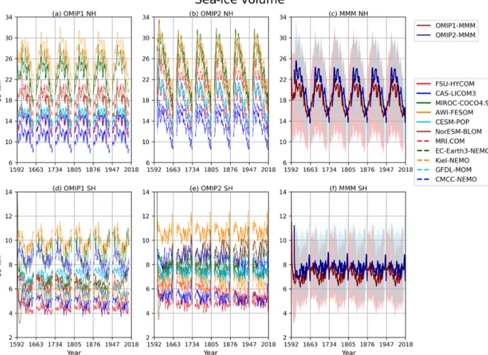
Long-term drift of sea ice is also a useful metric to assess steadiness of the simulated ocean–sea-ice system. Figure 4 shows the drift of ensemble mean sea-ice volume integrated

over each hemisphere. Notable drifts are not seen after the second cycle in the ensemble means. Also, the model spread does not show large variation, indicating that individual models do not have major drift or collapse of the sea-ice distribution (e.g., formation of open-ocean polynyas) by the end of the spin-up. The ranges of model spreads are very wide, with ratios of the maximum to the minimum reaching a fac- tor of 2–3, although these ranges may change slightly when we compare total sea-ice masses, which are obtained by mul- tiplying sea-ice density defined by each model to sea-ice vol- umes. Note that OMIP-2 simulations have larger sea-ice volume than OMIP-1 simulations in both hemispheres.

In contrast to heat content, the total salt content in the ocean–sea-ice system is essentially constant in nature.

In most participating models, the global salt content in the ocean–sea-ice system is explicitly conserved, which is achieved by removing the globally integrated salt flux aris- ing from salinity restoring at each time step (salinity normalization) as noted earlier. The same adjustment is applied to surface freshwater flux in most participating models, result-

(9)

Figure 3.Globally averaged drift of multi-model mean horizontal mean(a, c)temperature (^◦C) and(e, g)salinity (psu) as a function of depth and time. The drift is defined as the deviation from the annual mean of the initial year of the simulation by each model. For each, time evolution of the standard deviation of the model ensemble is depicted to the right.(a, b)OMIP-1 temperature,(c, d)OMIP-2 temperature, (e, f)OMIP-1 salinity, and(g, h)OMIP-2 salinity. See Figs. S3–S6 for results of individual models.

ing in conservation of total mass of water in the ocean–sea- ice system. Thus, in such models, variation of global mean salinity only occurs due to variation of sea-ice volume and the global mean salinity would not be normally employed as a metric for the purpose of model intercomparison. Figure 4 implies that global mean salinity increases for the first 10–

15 years of each forcing cycle and then decreases for the rest of the cycle in both the OMIP-1 and OMIP-2 simulations.

It also implies that a long-term drift of global mean salinity does not occur in those models that have applied both salinity and freshwater normalization.

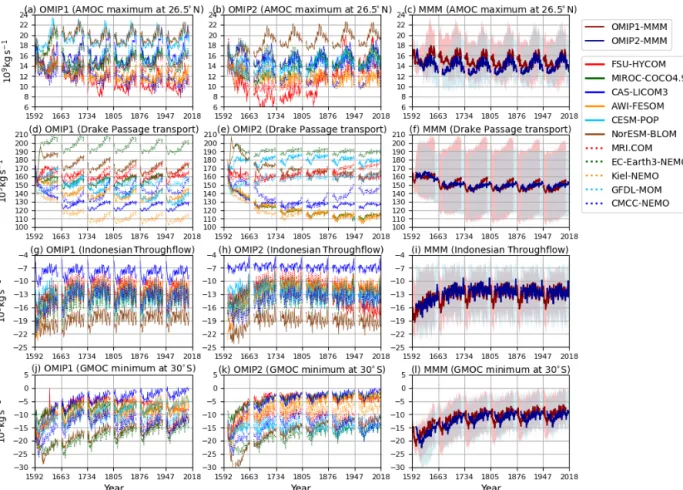
Figure 5 shows the time series for key circulation metrics, with Table D2 listing 1980–2009 means of the last cycle for all participating models. The AMOC at 26.5^◦N (defined as the vertical maximum of the streamfunction; Fig. 5a–c), which approximately represents the strength of AMOC associated with the North Atlantic Deep Water formation, shows little drift between cycles in OMIP-1 while it declines in the first cycle and slowly recovers thereafter in OMIP-2. This contrasting behavior is more clearly recognized by compar-

ing plots for all participating models of OMIP-1 and OMIP-2 (Fig. 5a and b, respectively). This initial decline of AMOC in many OMIP-2 simulations is at least partly caused by the larger amount of the mean freshwater discharge from Green- land in the OMIP-2 than the OMIP-1 dataset as described by Tsujino et al. (2018) (see their Fig. 20). This behavior ne- cessitates the six-cycle protocol for OMIP-2, which makes the period from fourth to sixth cycles suitable for studying the ocean uptake and spread of anthropogenic greenhouse gases (1850 to present) in OMIP-2. Drake Passage transport (Fig. 5d–f; positive transport eastward), which measures the strength of the Antarctic Circumpolar Current, shows quite similar behavior between OMIP-1 and OMIP-2 in terms of spin-up and strength, although the model spread is quite large. Drifts become small approximately after the fourth cycle. The same is true for Indonesian Throughflow (Fig. 5g–i;

negative transport into the Indian Ocean), which measures water exchange between the Pacific and Indian Ocean. The long-term drift seen in the first few cycles implies that the Indonesian Throughflow, largely constrained by the topog-

(10)

Figure 4.Time series of annual mean sea-ice volume integrated over the Northern Hemisphere (upper panels) and the Southern Hemisphere (lower panels):(a, d)OMIP-1 and(b, e)OMIP-2.(c, f)Multi-model mean (lines) and spread defined as the range between maximum and minimum (shades) of OMIP-1 (red) and OMIP-2 (blue). Units are 10³km³. See Fig. S7 for a closer look at individual models.

raphy and wind forcing, is also affected by the long-term thermohaline adjustment of the Indian and Pacific oceans (e.g., Sasaki et al., 2018). The global meridional overturning circulation (GMOC) minimum between 2000 m and the bottom at 30^◦S (Fig. 5j–l), which represents the strength of deep GMOC associated with the Antarctic Bottom Water and Lower Circumpolar Deep Water formation, shows a decreasing trend in the first few cycles but becomes persistent between forcing cycles after approximately the third cycle. The deep GMOC is slightly stronger in OMIP-2 simulations than OMIP-1 simulations, partly explaining the stronger cool- ing between 2000 m and the bottom in OMIP-2 simulations (Fig. 2i).

Summary of spin-up behavior

To summarize the spin-up behavior, OMIP-1 simulations take about three cycles to spin up, while OMIP-2 simulations take about four cycles. This behavior motivates the six-cycle integration for OMIP-2 simulations. Regarding OMIP-1, the fifth and sixth cycles show no major difference in the circulation metrics considered in this section except for the deep to

bottom layer temperature and salinity. This fact justifies the inclusion of five-cycle OMIP-1 simulations to the intercomparison of the “last cycle” as an evaluation of the contemporary climate of individual models as part of the remainder of our assessment.

The overall features of the simulated fields are quite similar between OMIP-1 and OMIP-2, except for some minor differences. Long-term drifts remain in the deep to bottom layer temperature and salinity even in the last cycle of simulations.

The deep ocean data from these simulations should be used with care as discussed by Doney et al. (2007). OMIP-2 simulations slightly deteriorate relative to OMIP-1 simulations in some metrics (e.g., warmer upper layer and initial decline of AMOC) and give larger model spreads in temperature and salinity. We expect simulation results to improve as experi- ences with the OMIP-2 dataset, including refinements to the model configurations, are accumulated and shared among the modeling groups.

(11)

Figure 5.Time series of annual mean ocean circulation metrics.(a–c)AMOC maximum at 26.5^◦N, which approximately represents the strength of AMOC associated with the North Atlantic Deep Water formation.(d–f)Drake Passage transport (positive eastward), which represents the strength of Antarctic Circumpolar Current.(g–i)Indonesian Throughflow (negative into the Indian Ocean), which represents water exchange between the Pacific and Indian oceans. (j–l)Global meridional overturning circulation (GMOC) minimum in 2000 m–

bottom depths at 30^◦S, which represents the strength of deep to bottom layer GMOC associated with the Antarctic Bottom Water and Lower Circumpolar Deep Water formation.(a, d, g, j)OMIP-1 and(b, e, h, k)OMIP-2.(c, f, i, l)Multi-model mean (lines) and spread defined as the range between maximum and minimum (shades) of OMIP-1 (red) and OMIP-2 (blue). Units are 10⁹kg s⁻¹. See Figs. S8 and S9 for a closer look at individual models.

4 Evaluation of contemporary climate of the last forcing cycle

We compare the contemporary climate of OMIP-1 and OMIP-2 simulations by focusing on the behavior of the multi-model ensemble mean. Here, we use the last cycle of all 11 participating models. These include simulations that performed OMIP-1 for five cycles and simulations that used slightly shorter periods (by 1–2 years) for forcing cycles before the last cycle. As shown in the previous section and Ap- pendix B1, for OMIP-1 simulations, the fifth and sixth cycles show no major differences in most metrics except for the deep layer temperature and salinity. Also, a minor difference in the total spin-up period does not result in a major difference in the contemporary climate of the last cycle.

Let us start by looking at sea surface temperature and salinity. Figures 6 and 7 show the ensemble mean bias, en-

semble standard deviation, and difference between OMIP- 1 and OMIP-2 simulations for the sea surface temperature and salinity, respectively, with Table D3 listing the root mean square bias and mean bias of the long-term average (1980–

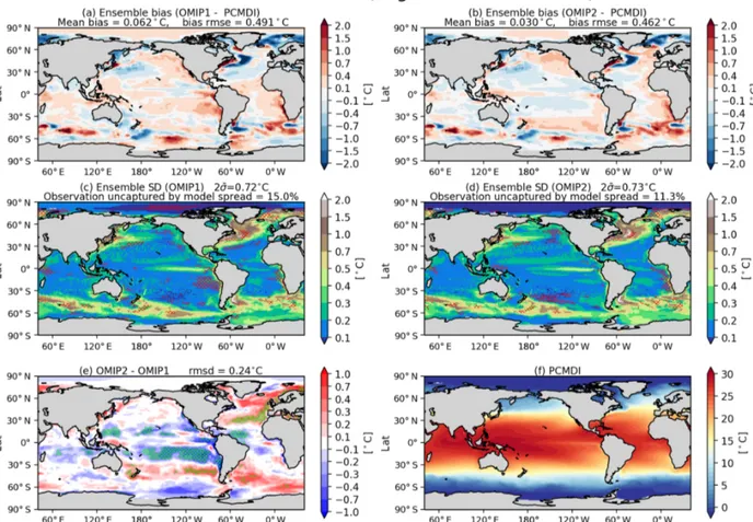
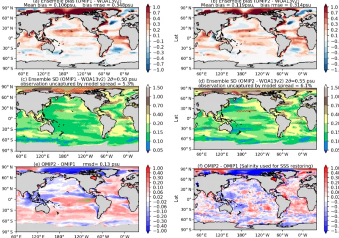
2009) of all participating models. The overall bias patterns of sea surface temperature are similar between OMIP-1 and OMIP-2, with the magnitude of the biases less than 0.4^◦C in most regions and with root mean square error (RMSE) of OMIP-2 reduced from OMIP-1 by about 6 %. However, the modeled confidence range given by twice the ensemble standard deviation is greater than the root mean square bias, with the observations captured by the modeled confidence range in more than 85 % of the region. The same is true for salinity, with the magnitude of the biases less than 0.4 practical salinity units (psu) in most regions. Note that the bias of OMIP-2 may have been underestimated relative to OMIP-1 because the salinity to which sea surface salinity

(12)

3654 H. Tsujino et al.: Evaluation of global ocean–sea-ice model simulations is restored in OMIP-2 is based on WOA13v2, which is also

used as the reference dataset for the evaluation. The ensemble spreads capture the observations in more than 90 % of the region. Note that the multi-model ensemble mean gives root mean square errors smaller than any individual models in both OMIP-1 and OMIP-2 simulations as shown in Ta- ble D3 in Appendix D and Figs. S10 and S11, a feature al- ready reported from the early stage of the climate model intercomparison activities (e.g., Lambert and Boer, 2001). It is also the case for sea surface salinity (Figs. S13 and S14) and sea surface height (SSH) (Figs. S24 and S25), except for sea surface height of GFDL-MOM, which performs better than the ensemble mean. Looking regionally, the warm biases and the high salinity biases around the eastern boundary upwelling region in the Pacific basin, specifically off Califor- nia and Chile, seen in OMIP-1, are reduced in OMIP-2. It is also the case for the eastern boundary region in the Atlantic basin, but the warm bias is somewhat exacerbated offshore in OMIP-2. The biases related to strong oceanic currents such as the western boundary currents, Antarctic Circum- polar Current, and Agulhas Current are common between OMIP-1 and OMIP-2. These biases are presumably caused by the relatively coarse horizontal resolution of the models, leading to poor reproducibility of the speed and locations of those currents and the resulting change of material distributions. In a companion paper (Chassignet et al., 2020), we will see how refined horizontal resolution is able to reduce these biases. The ensemble spread is large in the strong current regions, which are also the region with a large horizontal sea surface temperature gradient (a.k.a. fronts). The spread is also large in the marginal sea-ice zones.

Salinity tends to be higher in the Southern Hemisphere in OMIP-2, which results in either a reduction or increase of biases depending on locations. Both OMIP-1 and OMIP-2 simulations show high salinity bias in the Arctic Ocean, with some reduction implied for OMIP-2 simulations. The reduction of high salinity bias in the Arctic Ocean in OMIP-2 is partly explained by the difference in salinity to which sea surface salinity is restored between OMIP-2 (WOA13v2) and OMIP-1 (PHC; Steele et al., 2001) as shown in Fig. 7f. Note that the Arctic Ocean has shown a strong freshening trend over recent decades (Rabe et al., 2014; Wang et al., 2019);

thus, restoring sea surface salinity to the climatology in the models may result in high salinity biases in recent years.

The model spread of salinity is large in the Arctic Ocean, where the diversity among models in the sea-ice processes, the surface vertical mixing processes, and the treatment of salinity restoring can lead to large difference in sea surface salinity. The model spread is also large in the region around the mouths of large rivers such as the Amazon, Yangtze, and Ganges, indicating that the ways the freshwater from rivers is distributed in the models are quite diverse.

How do these bias patterns found after a long-term model integration for sea surface temperature and salinity appear in the initial years of the integration? Figure 8 compares bi-

ases for the initial 5-year mean and the long-term mean of the last cycle from the OMIP-2 simulation of MRI.COM.

Some notable biases of sea surface temperature such as the warm bias in the eastern boundary of the South Atlantic and the cold bias in the midlatitude western North Pacific are al- ready found in the initial years. When the salinity in the later years is subtracted by its global mean, overall spatial patterns of salinity bias are similar between the initial years and the later years. (Note that the global mean sea surface salinity of MRI.COM is gradually increasing throughout the integration as shown in Fig. 1g.) This behavior may not necessarily ap- ply to other metrics, but these results for sea surface temperature and salinity indicate that a short-term integration can be useful for detecting and attributing causes of some biases.

Sea ice is also an important metric since it comprises the boundary condition for other components of the Earth system models, with Fig. 9 presenting an assessment of sea-ice distribution. In Northern Hemisphere winter (top panels), both OMIP-1 and OMIP-2 reproduce the observed distribution of sea-ice concentration reasonably well. But the sea ice covers a wider area than the observation in the Greenland–Iceland–

Norwegian seas. In Northern Hemisphere summer (second row), OMIP-1 clearly underestimates sea-ice concentration, which is improved in OMIP-2, although the sea-ice extent is similar for the two simulations. In the Southern Hemisphere, again, both OMIP-1 and OMIP-2 reproduce the observed distribution reasonably well in winter (third row), with OMIP- 2 generally giving a smaller sea-ice extent than OMIP-1. In summer (bottom row), OMIP-2 reduces the low concentration bias in OMIP-1, thus giving a more realistic sea-ice extent in OMIP-2.

The sea surface height, or ocean dynamic sea level, represents dynamical properties of the ocean, with its horizontal gradient balancing the geostrophic current near the sea surface. Figure 10 presents an assessment of sea surface height, with Table D3 listing the root mean square bias of the 1993–2009 mean sea surface height for all participating models. Note that Appendix C details the preprocessing necessary to compare sea surface heights from observation and simulations. The overall bias patterns are quite similar between OMIP-1 and OMIP-2 except for the north equatorial Pacific Ocean. A zonally elongated pattern of positive bias occurs from the western to central basin in OMIP-1 and from the central to eastern basin in OMIP-2. Both OMIP-1 and OMIP-2 ensemble spreads fail to capture the observation there (Fig. 10c and d). The issue is related to the wind stress field around the Intertropical Convergence Zone, which will be further discussed when exploring the North Equatorial Countercurrent later in this section (see Fig. 18). The positive anomaly in the northern North Pacific of OMIP-2 relative to OMIP-1 is presumably due to the known weaker wind stress in OMIP-2 relative to OMIP-1 (e.g., Taboada et al., 2019), which will be discussed in relation to meridional overturning circulations and northward heat transport later in this section (see Figs. 15–17). The zonally elongated pattern of

(13)

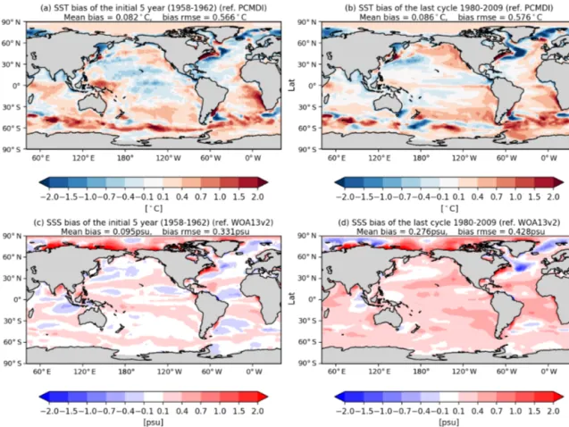
Figure 6.Evaluation of the simulated mean sea surface temperature (SST; units in^◦C). Panels(a)and(b)show the bias of the multi-model mean, 30-year (1980–2009) mean SST relative to an observational estimate provided and updated by Program for Climate Model Diagnosis and Intercomparison (PCMDI) following a procedure described by Hurrell et al. (2008) (hereafter referred to as PCMDI-SST).(a)OMIP-1 and(b)OMIP-2, with global mean bias and global root mean square bias depicted at the top. The middle two panels show the standard deviation of the ensemble, with the regions where the observation is outside the 95 % confidence range of the model spread (±2σ) hatched with red.(c)OMIP-1 and(d)OMIP-2, with the global mean confidence range (twice the standard deviation) and the fraction of the region where observation is uncaptured by the model confidence range depicted at the top.(e)Difference between OMIP-1 and OMIP-2 (OMIP-2 minus OMIP-1), with the global root mean square difference depicted at the top. The regions where the difference is significant at 95 % confidence level are hatched with green, with the uncertainty of multi-model mean difference computed based on the method proposed by Wakamatsu et al. (2017).(f) The 30-year (1980–2009) mean SST of PCMDI-SST. In the following figures, all models are used for multi-model mean. See Figs. S10–S12 for results of individual models.

negative and positive biases found along the Kuroshio Ex- tension to the east of Japan is presumably due to the lack of twin recirculation gyres along the Kuroshio Extension in low-resolution models (e.g., Qiu et al., 2008; Nakano et al., 2008). The negative bias found along the Gulf Stream extension implies the failure of the models to reproduce the Gulf Stream penetration and associated recirculation gyres.

The reason for that failure would not be simple because the western boundary current, the deep water formation, and the bottom topography interact to form the mean state, with very fine (∼1/50^◦) horizontal resolution models generally required to reduce the biases (e.g., Chassignet and Xu, 2017).

A large difference in sea surface height is found in the eastern Arctic Ocean, with OMIP-2 higher than OMIP-1. This difference is presumably related to the lower upper ocean salinity

(and thus less dense water) found in OMIP-2 (Fig. 7e). Note that the inter-model spread is similar between OMIP-1 and OMIP-2, with large spread found in the strong current regions.

Seasonal evolutions of the surface mixed layer depths determine the way the ocean interior is ventilated. The annual maximum and minimum occurring in winter and summer, respectively, are particularly important metrics. Note that the definition for mixed layer depth used in OMIP is explained in Appendix H24 of Griffies et al. (2016). Specifically, mixed layer depth is determined based on the vertical distribution of a buoyancy difference,δB, computed as

δB= −g ρdisplaced from surface−ρ_local

/ρ_local, (1)

where

(14)

Figure 7.Evaluation of simulated sea surface salinity (SSS; units in psu). Panels(a)and(b)show the bias of the multi-model mean 30-year (1980–2009) mean SSS relative to WOA13v2 (Zweng et al., 2013).(a)OMIP-1 and(b)OMIP-2. The middle two panels show the standard deviation of the ensemble, with the regions where the observation is outside the 95 % confidence range of the model spread (±2σ) hatched with red.(c)OMIP-1 and(d)OMIP-2.(e)Difference between OMIP-1 and OMIP-2 (OMIP-2 minus OMIP-1), with the regions where the difference is significant at 95 % confidence level hatched with green as in Fig. 6.(f)Difference of salinity to which sea surface salinity is restored in OMIP-1 and OMIP-2 (OMIP-2 minus OMIP-1). At the top of each panel, global mean values are depicted as in Fig. 6. See Figs. S13–S15 for results of individual models.

ρdisplaced from surface=ρ

S (k=1) , 2 (k=1) , p(k) andρ_local=ρ

S (k) , 2 (k) , p(k)

, (2)

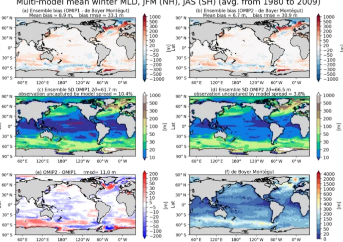
with salinity, temperature, and pressure represented by S, 2, and p, respectively. The mixed layer depth is approx- imated as the first depth from the surface where δB= 1Bcrit=0.0003 m s⁻²using any kind of interpolation. Note that 1Bcrit=0.0003 m s⁻²corresponds to a critical density difference of1ρcrit=0.03 kg m⁻³, which is adopted by the observational dataset compiled by de Boyer Montégut et al. (2004) used for the present evaluation. Figures 11 and 12 show the biases of the winter and summer mixed layer depth in both hemispheres, respectively, with Table D4 listing the root mean square bias and mean bias of the 1980–

2009 mean for all participating models. Both OMIP-1 and OMIP-2 biases exhibit similar horizontal distributions with OMIP-2 showing smaller root mean square errors. In winter,

mixed layer depths of a few hundred meters are formed in the midlatitude western boundary current extension regions such as the Kuroshio Extension and the Gulf Stream extension.

Mixed layer depths of more than 1000 m are formed in the Weddell Sea, the Labrador Sea, and the Greenland–Iceland–

Norwegian seas, where deep and bottom waters are formed in the models. Models tend to show deeper bias in both regions, also exhibiting a large model spread. The mixed layer depth is deeper in the Labrador and Irminger seas in OMIP-2 than OMIP-1. Around Greenland, the mixed layer is shallower in OMIP-2 than OMIP-1, which is presumably caused by the larger freshwater discharge from Greenland in the OMIP-2 (JRA55-do) dataset. The lower sea surface salinity of OMIP- 2 shown in Fig. 7e is also consistent with its shallower mixed layer. The rather deep mixed layer in the modeled Weddell Sea is not found in observations (though observations are rather limited in this region) and may represent an unrealistic formation process of the simulated Antarctic Bottom Water.

(15)

Figure 8.Comparison of SST(a, b)and SSS(c, d)biases relative to observations (PCMDI-SST and WOA13v2, respectively) for the initial 5-year mean(a, c)and the long-term mean (1980–2009) in the last cycle(b, d)from the OMIP-2 simulation of MRI.COM. Pattern correlation of biases between the initial 5-year mean and the long-term mean in the last cycle is 0.75 for SST and 0.85 for SSS.

In summer, both OMIP-1 and OMIP-2 exhibit biases less than 10 m in most regions, implying that the observational estimates are well reproduced. One notable exception is that the summer mixed layer depth in OMIP-2 is deeper by about 10 m around the Antarctic Circumpolar Current region, with the OMIP-2 behavior closer to observational estimates.

Model spreads of OMIP-1 and OMIP-2 are also similar.

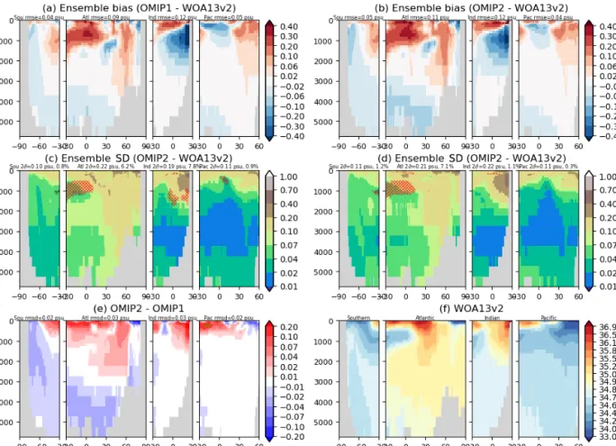
We will proceed with the evaluation toward the ocean interior. Figures 13 and 14 show the basin-wide zonal mean temperature and salinity, respectively, with Tables D5 and D6 listing the root mean square bias of the 1980–2009 mean of temperature and salinity for all participating models. First, it is notable that the bias patterns of OMIP-1 and OMIP-2 are similar. Also note that the biases of temperature and salinity show very similar patterns, thus indicating that they are compensating each other in their effects on density biases (small density biases can be expected). The cold and fresh biases in the 1000–2000 m depth range of the northern In- dian Ocean and the subsurface South Pacific seen in OMIP-1 are reduced in OMIP-2, while the warm and salty bias in the 2000–3000 m depth range and the cold and fresh bias in the bottom of the Atlantic Ocean in OMIP-1 are slightly exac-

erbated in OMIP-2. Note that large model spreads are found for the cold and fresh biases in the 1000–2000 m depth range of the northern Indian Ocean and the warm and salty bias in the 1000–3000 m depth range in the high-latitude North Atlantic Ocean. These are the regions where an exchange of water masses occurs between an oceanic basin and marginal seas through oceanic sills (between the Indian Ocean and Red Sea/Persian Gulf and between the Atlantic Ocean and Greenland–Iceland–Norwegian seas). Models show diverse behavior according to the representation of topography and the parameterization of unresolved mixing and transport.

Bottom water temperature shows a model spread (∼0.5–

1^◦C) larger than the difference between OMIP-1 and OMIP- 2 in all basins (∼0.1^◦C). The model spread for bottom water salinity shows different patterns than those of temperature, but the model spread for bottom water salinity is larger than the difference of salinity between OMIP-1 and OMIP-2 in all basins.

The basin-wide averaged material distributions and thus important climate metrics such as the meridional heat transport are largely determined by the meridional overturning circulations, with Fig. 15 showing the stream functions

(16)

Figure 9.Multi-model mean 30-year (1980–2009) mean sea-ice concentration (%). Columns are (from the left) OMIP-1, OMIP-2, OMIP- 2−OMIP-1, and an observational dataset provided by PCMDI-SST. Rows are (from the top) March and September in the Northern Hemi- sphere, and September and March in the Southern Hemisphere. Blue lines are contours of 15 % concentration of the PCMDI-SST dataset and red lines are those of multi-model mean. See Figs. S16–S23 for results of individual models.

of basin-wide meridional overturning circulations. The difference between OMIP-1 and OMIP-2 is less than 1 Sv (1 Sv=10⁶m³s⁻¹) in most regions. The subtropical cells in the upper layer of the Indo-Pacific sector and the clockwise cell in the Southern Ocean sector are weaker in OMIP-2, which is presumably due to the known weaker wind stress in OMIP-2 relative to OMIP-1 (e.g., Taboada et al., 2019).

The upper counterclockwise cell in the mid- to high-latitude North Pacific sector is also weaker in OMIP-2. Figure 16 shows the multi-model mean, basin-wide averaged zonal wind stress for OMIP-1 and OMIP-2. The zonal wind stress

of OMIP-2 is weaker than OMIP-1, but OMIP-2 is closer to observational estimates. This difference is due to the difference in the treatment of equivalent neutral wind between the OMIP-1 and OMIP-2 datasets as explained by Tsujino et al. (2018). The model spreads of meridional overturning circulations (Fig. 15c and d) are large in the maximum and minimum of major meridional overturning circulation cells that represent the thermohaline circulations, whereas the model spreads are relatively small in the upper few hundred meters presumably because the upper ocean meridional overturning circulation cells are dynamically constrained by the

(17)

Figure 10.Evaluation of simulated sea surface height (m). Panels(a)and(b)show the bias of the multi-model mean, 17-year (1993–2009) mean SSH relative to the Copernicus Marine Environment Monitoring Service (CMEMS).(a)OMIP-1 and(b)OMIP-2. The middle two panels show the standard deviation of the ensemble, with the regions where the observation is outside the 95 % confidence range of the model spread (±2σ) hatched with red.(c)OMIP-1 and(d)OMIP-2.(e)Difference between OMIP-1 and OMIP-2 (OMIP-2 minus OMIP-1), with the regions where the difference is significant at 95 % confidence level hatched with green as in Fig. 6.(f)Annual mean SSH of CMEMS.

Note that all SSH fields are offset by subtracting their respective quasi-global mean values before evaluation as described in Appendix C. At the top of each panel, global mean values are depicted as in Fig. 6. See Figs. S24–S26 for results of individual models.

surface wind stress. Note that the large model spreads near the surface in the Southern Ocean (north of ∼60^◦S) and over the tropical cells in the Indo-Pacific Ocean are likely due to differences in the implementation and the parameters for the eddy-induced transport parameterizations in models, with details given in Appendix A and references therein.

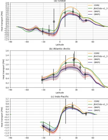
The northward heat transport is assessed in Fig. 17. Al- though both OMIP-1 and OMIP-2 are largely within the uncertainty range of observational estimates, northward heat transport in the Atlantic Ocean is significantly smaller than the observational estimates at 26.5^◦N in both cases and OMIP-2 is smaller than OMIP-1 almost everywhere. Note that a recent estimate by Trenberth and Fasullo (2017) gives around 1.0±0.1 PW for the peak value of the North Atlantic, which overlaps better with the OMIP-1 and OMIP-2 enve- lope. The difference between OMIP-1 and OMIP-2 simulations is qualitatively consistent with the implied northward heat transport of OMIP-1 and OMIP-2 forcing datasets (Tsu- jino et al., 2018). The difference is presumably attributed

to the known weaker wind speed of OMIP-2 (e.g., Taboada et al., 2019) as explained earlier in this section. The cool- ing near the surface in the tropical North Pacific Ocean and warming below in OMIP-2 relative to OMIP-1 for the zonally averaged temperatures as shown in Fig. 13e further weakens the northward heat transport in the North Pacific in OMIP-2, though it is notable that these changes reduce the temperature biases in OMIP-2.

In the tropical Pacific Ocean, mean surface and subsurface zonal currents can reach more than several tens of cm s⁻¹ (Johnson et al., 2002), and thus they can have non-trivial impact on material circulations and distributions in this region. In particular, the collective effect of the climatologi- cal currents on the advection of anomalous temperature is to dampen growth of El Ninõ–Southern Oscillation (ENSO) (Jin et al., 2006; Kim and Jin, 2011) and the mean currents are thought to be important to characterize the representation of ENSO in coupled models (Bellenger et al., 2014).

Figure 18 shows the zonal velocity across a latitude–depth

(18)

Figure 11.Evaluation of simulated mixed layer depth (m). Panels(a)and(b)show the bias of the multi-model mean, 30-year (1980–2009) mean winter mixed layer depth in both hemispheres relative to observationally derived mixed layer depth data from de Boyer Montégut et al. (2004). January–February–March mean for the Northern Hemisphere and July–August–September mean for the Southern Hemisphere.

(a)OMIP-1 and(b)OMIP-2. The middle two panels show the standard deviation of the ensemble, with the regions where the observation is outside the 95 % confidence range of the model spread (±2σ) hatched with red.(c)OMIP-1 and(d)OMIP-2.(e)Difference between OMIP-1 and OMIP-2 (OMIP-2 minus OMIP-1), which is not statistically significant at 95 % confidence level everywhere.(f)Observationally derived mixed layer depth data from de Boyer Montégut et al. (2004). At the top of each panel, global mean values are depicted as in Fig. 6. Note that the regions where mixed layer depths could reach more than 1000 m in winter, specifically the marginal seas around Antarctica (south of 60^◦S) and the high-latitude North Atlantic (50–80^◦N; 80^◦W–30^◦E), are excluded from the computation of global means. See Figs. S27–S29 for results of individual models.

section along 140^◦W of the eastern tropical Pacific Ocean.

The eastward Equatorial Undercurrent around 100 m depth and the westward South Equatorial Current at the surface are reproduced well in both simulations. However, as reported by Tseng et al. (2016), the surface eastward current of the North Equatorial Countercurrent at 6–8^◦N is weak in OMIP- 1 simulations. This bias has been improved only slightly in OMIP-2 simulations. The reason for this bias is presumably related to the method used to adjust the wind vector in both OMIP-1 (CORE-II) and OMIP-2 (JRA55-do) forcing fields as noted by Z. Sun et al. (2019). The weak wind variabilities in the Intertropical Convergence Zone (ITCZ) in the original reanalysis products have been adjusted by increasing the wind speed in both forcing datasets (see Fig. 10 of Tsujino et al., 2018). This wind speed increase results in the erroneous strengthening of the weaker mean easterly wind along

the ITCZ relative to its surroundings, which was reproduced rather realistically in the original JRA-55 reanalysis. The result after the adjustment is a shallowing of the minimum of the mean easterly winds along the ITCZ and a weakening of the wind stress curl both north and south of the ITCZ, leading to a weakening of the eastward North Equatorial Counter- current and bias in the sea surface height shown in Fig. 10.

Note also that the strengthening of the easterly wind over the surface eastward current of the North Equatorial Coun- tercurrent results in the weakening of the eastward current in the simulations because the wind stress further weakens the current as shown by Yu et al. (2000). As a final note, the majority of participating models with horizontal resolution around 1^◦fail to reproduce the subsurface eastward currents in the 200–300 m depth range both north and south of the Equator (a.k.a. Tsuchiya jets; Tsuchiya, 1972, 1975). Ishida