simulations based on the experimental protocols of the Ocean Model Intercomparison Project phase 2 (OMIP-2)

(1)

Geosci. Model Dev., 13, 4595–4637, 2020 https://doi.org/10.5194/gmd-13-4595-2020

Impact of horizontal resolution on global ocean–sea ice model

simulations based on the experimental protocols of the Ocean Model Intercomparison Project phase 2 (OMIP-2)

Eric P. Chassignet¹, Stephen G. Yeager², Baylor Fox-Kemper³, Alexandra Bozec¹, Frederic Castruccio², Gokhan Danabasoglu², Christopher Horvat³, Who M. Kim², Nikolay Koldunov⁴, Yiwen Li⁵, Pengfei Lin⁵, Hailong Liu⁵, Dmitry V. Sein^4,6, Dmitry Sidorenko⁴, Qiang Wang⁴, and Xiaobiao Xu¹

1Center for Ocean–Atmospheric Prediction Studies, Florida State University, Tallahassee, FL, USA

2National Center for Atmospheric Research, Boulder, CO, USA

3Brown University, Providence, RI, USA

4Alfred-Wegener-Institut Helmholtz-Zentrum für Polar- und Meeresforschung (AWI), Bremerhaven, Germany

5State Key Laboratory of Numerical Modeling for Atmospheric Sciences and Geophysical Fluid Dynamics, Institute of Atmospheric Physics, Chinese Academy of Sciences, Beijing, China

6Shirshov Institute of Oceanology, Russian Academy of Science, Moscow, Russia Correspondence:Eric P. Chassignet (echassignet@fsu.edu)

Received: 31 December 2019 – Discussion started: 11 March 2020

Revised: 9 August 2020 – Accepted: 15 August 2020 – Published: 29 September 2020

Abstract.This paper presents global comparisons of fundamental global climate variables from a suite of four pairs of matched low- and high-resolution ocean and sea ice simulations that are obtained following the OMIP-2 protocol (Griffies et al., 2016) and integrated for one cycle (1958–

2018) of the JRA55-do atmospheric state and runoff dataset (Tsujino et al., 2018). Our goal is to assess the robustness of climate-relevant improvements in ocean simulations (mean and variability) associated with moving from coarse (∼1^◦) to eddy-resolving (∼0.1^◦) horizontal resolutions. The models are diverse in their numerics and parameterizations, but each low-resolution and high-resolution pair of models is matched so as to isolate, to the extent possible, the effects of horizontal resolution. A variety of observational datasets are used to assess the fidelity of simulated temperature and salinity, sea surface height, kinetic energy, heat and volume transports, and sea ice distribution. This paper provides a crucial bench- mark for future studies comparing and improving different schemes in any of the models used in this study or similar ones. The biases in the low-resolution simulations are famil- iar, and their gross features – position, strength, and variability of western boundary currents, equatorial currents, and the Antarctic Circumpolar Current – are significantly improved

in the high-resolution models. However, despite the fact that the high-resolution models “resolve” most of these features, the improvements in temperature and salinity are inconsis- tent among the different model families, and some regions show increased bias over their low-resolution counterparts.

Greatly enhanced horizontal resolution does not deliver unambiguous bias improvement in all regions for all models.

1 Introduction

A key decision in climate model design is the spatial resolution of different components. The global scope of the inte- grations and the centennial to millennial timescales and mul- tiple scenarios required to capture changes in the climate set the problem; the spatial resolution is therefore the result of available computing. This decade, computing has become sufficiently powerful to make mesoscale-rich resolution af- fordable in ocean and sea ice models over most of the Earth, which allows the ocean model to simulate more intense in- ternal variability than a lower-resolution model. As this new regime of coupled modeling is entered, it is important to understand both the behavior of ocean and sea ice models in

(2)

4596 E. P. Chassignet et al.: OMIP-2 a controlled framework and the benefits and challenges that

come with higher resolution. This work introduces a set of matched numerical simulations in low- and high-resolution ocean and sea ice models with the latest forcing protocol.

It is anticipated that these results will inform fully coupled modeling studies wherein ocean resolution varies and also that follow-on studies will build on our results to examine process and regional detail.

In 2016, an international group of ocean modelers behind the development and analysis of global ocean–sea ice models used as a component of the Earth system models in CMIP6 proposed an Ocean Model Intercomparison Project (OMIP) (Griffies et al., 2016). The essential element behind the OMIP is a common set of atmospheric and river runoff datasets for computing surface boundary fluxes to drive the ocean–sea ice models, many of which are used as components of coupled climate system models. The OMIP protocol is an outcome of the Coordinated Ocean–ice Reference Experiments (COREs), which assessed the performance of ocean–sea ice models (Griffies et al., 2009, 2014; Danaba- soglu et al., 2014, 2016; Downes et al., 2015; Farneti et al., 2015; Wang et al., 2016a, b; Ilicak et al., 2016; Tseng et al., 2016; Rahaman et al., 2020) using the atmospheric and river runoff dataset of Large and Yeager (2009). However, this dataset has not been updated since 2009, and a new dataset (JRA55-do; Tsujino et al., 2018) has been developed for the OMIP based on the Japanese Reanalysis (JRA-55) product from Kobayashi et al. (2015) to ensure that it is regularly updated. This raw reanalysis product has been substantially adjusted to match reference states based on observations or the ensemble mean of other atmospheric reanalysis products as detailed in Tsujino et al. (2018) to create a suitable forcing dataset for ocean and sea ice models, referred to as JRA55- do. The continental river discharge is provided by a river- routing model forced by input runoff from the land surface component of JRA-55 adjusted to ensure similar long-term variabilities as in the CORE dataset (Suzuki et al., 2018).

Runoff from ice sheets and glaciers from Greenland (Bam- ber et al., 2012, 2018) and Antarctica (Depoorter et al., 2013) are also incorporated. Tsujino et al. (2020) present an evaluation of the simulations from CMIP6-class global ocean–

sea ice models forced with the JRA55-do datasets. This ef- fort compares CORE-forced (i.e., OMIP-1) and JRA55-do- forced (i.e., OMIP-2) simulations considering metrics com- monly used in the evaluation of global ocean–sea ice models to assess model biases.

Many features are very similar between OMIP-1 and OMIP-2 simulations, but Tsujino et al. (2020) identify many improvements in the simulated fields in transitioning from OMIP-1 to OMIP-2. For example, the sea surface temperature of the OMIP-2 simulations reproduces the global warming hiatus in the 2000s and the recent observed warming, which are absent in OMIP-1, partly because the OMIP-1 forcing stopped in 2009. The low bias in the sea ice area fraction in summer for both hemispheres in OMIP-1 is signif-

icantly improved in OMIP-2. The overall reproducibility of both seasonal and interannual variation in sea surface temperature and sea surface height (dynamic sea level) is also improved in OMIP-2. Tsujino et al. (2020) attribute many of the remaining model biases either to errors in representing important processes in ocean–sea ice models, some of which are expected to be mitigated by taking finer horizontal and/or vertical resolutions, or to shared biases in the atmospheric forcing. In this paper, we make a first attempt at quantifying the impacts of the models’ horizontal resolution on biases.

Our goal is to assess the robustness of climate-relevant improvements in ocean simulations (mean and variability) associated with moving from coarse (∼1^◦) to eddy-resolving (∼0.1^◦) horizontal resolutions. Using the same atmospheric forcing (JRA55-do) for both low- and high-resolution configurations, we perform a multi-model analysis to identify the robust differences and improvements associated with increased resolution given the same forcing datasets. Within the ocean modeling community, it is usually assumed that high-resolution simulations should in general produce better results than low-resolution ones (Fox-Kemper et al., 2019).

While this is clearly the case for surface currents and inter- nal variability, we will show that greatly enhanced horizontal resolution does not necessarily deliver unambiguous bias improvement in temperature and salinity in all regions. It is important to note several caveats when interpreting the results presented in this paper: first, this is based on a limited number of numerical models (four), and second, because of the large computational cost associated with the high-resolution runs (factor of 1000 more expensive), only one JRA55-do cycle (1958–2018) is analyzed in this paper (versus six cycles for the coarse-resolution runs of Tsujino et al., 2020). Also, because of the short integration time, some of the results may not be robust (Atlantic meridional overturning circulation variability, deep-ocean circulation, etc.) (Danabasoglu et al., 2016). The layout of the paper is as follows. The models used in the comparison are described in Sect. 2. Section 3 highlights differences in the magnitude of the models’ drift, while Sect. 4 focuses on the detrended interannual to decadal variability and the differences in the modeled ocean climates.

The results are summarized and discussed in the final section.

2 Description of the models

The CMIP6 OMIP-2 protocol does not include any spec- ifications regarding model resolution, but most participat- ing groups employ ocean models with horizontal resolution (∼1^◦) similar to what is used in the CMIP6 DECK experiments (Eyring et al., 2016) in order to achieve the required five-cycle spin-up (Tsujino et al., 2020). A high-resolution version of OMIP-2, with no multi-cycle spin-up requirement or well-defined protocols apart from the use of JRA55-do forcing, was informally organized by the CLIVAR Ocean Model Development Panel (OMDP) in 2019 to leverage the

(3)

E. P. Chassignet et al.: OMIP-2 4597

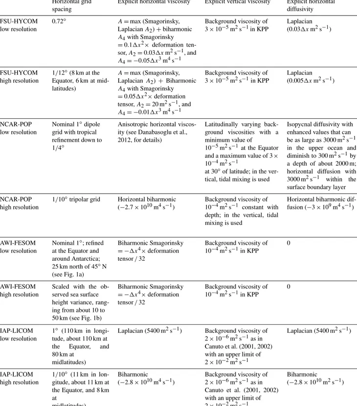
Table 1.Model parameters for the low- and high-resolution configurations.

Horizontal grid spacing

Explicit horizontal viscosity Explicit vertical viscosity Explicit horizontal diffusivity FSU-HYCOM

low resolution

0.72^◦ A=max (Smagorinsky,

LaplacianA₂)+biharmonic A₄with Smagorinsky

=0.11x²×deformation tensor,A₂=0.031xm²s⁻¹, and A₄= −0.051x³m⁴s⁻¹

Background viscosity of 3×10⁻⁵m²s⁻¹in KPP

Laplacian (0.031xm²s⁻¹)

FSU-HYCOM high resolution

1/12^◦(8 km at the Equator, 6 km at midlatitudes)

A=max (Smagorinsky, Laplacian A₂) +Biharmonic A₄with Smagorinsky

=0.051x²×deformation tensor,A₂=20 m²s⁻¹, and A₄= −0.011x³m⁴s⁻¹

Background viscosity of 3×10⁻⁵m²s⁻¹in KPP

Laplacian (0.0051xm²s⁻¹)

NCAR-POP low resolution

Nominal 1^◦dipole grid with tropical refinement down to 1/4^◦

Anisotropic horizontal viscosity (see Danabasoglu et al., 2012, for details)

Latitudinally varying background viscosities with a minimum value of

10⁻⁵m²s⁻¹ at the Equator and a maximum value of 3× 10⁻⁴m²s⁻¹

at 30^◦of latitude; in the vertical, tidal mixing is used

Isopycnal diffusivity with enhanced values that can be as large as 3000 m²s⁻¹ in the upper ocean and diminish to 300 m²s⁻¹by a depth of about 2000 m;

horizontal diffusion with 3000 m²s⁻¹ within the surface boundary layer NCAR-POP

high resolution

1/10^◦tripolar grid Horizontal biharmonic (−2.7×10¹⁰m⁴s⁻¹)

Background viscosity of 10⁻⁴m²s⁻¹ constant with depth; in the vertical, tidal mixing is used

Horizontal biharmonic diffusion (−3×10⁹m⁴s⁻¹)

AWI-FESOM low resolution

Nominal 1^◦; refined at the Equator and around Antarctica;

25 km north of 45^◦N (see Fig. 1a)

Biharmonic Smagorinsky

= −1x⁴×deformation tensor/32

Background viscosity of 10⁻⁴m²s⁻¹in KPP

0

AWI-FESOM high resolution

Scaled with the observed sea surface height variance, ranging from about 10 to 50 km (see Fig. 1b)

Biharmonic Smagorinsky

= −1x⁴×deformation tensor/32

Background viscosity of 10⁻⁴m²s⁻¹in KPP

0

IAP-LICOM low resolution

1^◦ (110 km in longitude, about 110 km at the Equator, and 80 km at

midlatitudes)

Laplacian (5400 m²s⁻¹) Background viscosity of 2×10⁻⁶m²s⁻¹as in Canuto et al. (2001, 2002) with an upper limit of 2×10⁻²m²s⁻¹

Laplacian (5400 m²s⁻¹)

IAP-LICOM high resolution

1/10^◦ (11 km in longitude, about 11 km at the Equator, and 8 km at

midlatitudes)

Biharmonic

(−2.8×10¹⁰m⁴s⁻¹)

Background viscosity of 2×10⁻⁶m²s⁻¹as in Canuto et al. (2001, 2002) with an upper limit of 2×10⁻²m²s⁻¹

Biharmonic

(−2.8×10¹⁰m²s⁻¹)

(4)

4598 E. P. Chassignet et al.: OMIP-2

Table 1.Continued.

Isopycnal scheme, e.g., GM

Mixed layer scheme

Momentum advection scheme

Tracer advection scheme

Time stepping scheme

FSU-HYCOM low resolution

Laplacian (0.011xm²s⁻¹) +biharmonic

(−0.021x³m⁴s⁻¹) thickness diffusion

KPP Second-order FCT Second-order FCT Split-explicit leapfrog with Asselin filter (0.125)

Biharmonic thickness diffusion (−0.0151x³m⁴s⁻¹)

KPP Second-order FCT Second-order FCT Split-explicit leapfrog with Asselin filter (0.125)

GM+submesoscale parameterization

KPP Second-order cen-

tered

Third-order upwind Second-order leapfrog

scheme with Asselin filter

NCAR-POP high resolution

None KPP Second-order cen-

tered

Second-order cen- tered

Second-order leapfrog

scheme with averag- ing time step AWI-FESOM

low resolution

Laplacian Redi and thickness diffusion, diffusivity flow-dependent in the range of 0 to 1500 m² as implemented in Danabasoglu et al. (2008)

KPP Taylor–Galerkin Second-order FCT Pressure split; implicit SSH

AWI-FESOM high resolution

Laplacian Redi and thickness diffusion, diffusivity- flow-dependent in the range of 0 to 1500 m² as implemented in Danabasoglu et al. (2008) and scaled with grid cell area

KPP Taylor–Galerkin Second-order FCT Pressure split; implicit SSH

IAP-LICOM low resolution

Both Redi and GM with coefficient computed as in Ferreira et al. (2005)

Canuto et al.

(2001, 2002)

Two-step preserving shape (Yu, 1994)

Split-explicit leapfrog with Asselin filter (0.2 for barotropic;

0.43 for baroclinic;

0.43 for tracer) IAP-LICOM

high resolution

None Canuto et al.

(2001, 2002)

Two-step preserving shape (Yu, 1994)

Split-explicit leapfrog with Asselin filter (0.2 for barotropic;

0.43 for baroclinic;

0.43 for tracer)

high-resolution (defined as being eddy-resolving over most of the globe, i.e., ∼1/10^◦) work already being carried out by several of the modeling groups involved in the OMDP (coupled and uncoupled configurations). This study is an “intercomparison of opportunity” made possible by the handful of groups that were able to run parallel JRA55-do simulations at both eddy-parameterized (low) and eddy-resolving (high) resolutions. The high-resolution experiments are com- putationally expensive, and, when the call for comparison was made, each group leveraged known and proven configurations to perform the requested experiments. Furthermore,

some groups had already completed the JRA55-do simulations at high resolution before this intercomparison was con- ceived. Given the large computational resources involved, re- running those experiments to conform to a standard protocol was not an option. All experiments were configured using best practices, but each modeling group was empowered to choose what they thought was best and configured their high- and low-resolution configurations with similar parameters (see Table 1 for a detailed description of the parameters used in the low- and high-resolution model configurations).

Ideally, only the horizontal resolution and associated physics

(5)

Table 1.Continued.

Bottom drag Surface

wind stress

Vertical coordinates

Initial conditions

SSS restoring

FSU-HYCOM low resolution

Quadratic bottom dragC_b(|U|+U_bar)U^* withC_b=1.5×10⁻³and

U_bar=0.05 m s⁻¹

Absolute 41 hybrid layers

GDEM4 30 m per 60 d to monthly GDEM4

Quadratic bottom dragC_b(|U|+U_bar)U^* withC_b=1.5×10⁻³and

U_bar=0.05 m s⁻¹

Absolute 36 hybrid layers

GDEM4 30 m per 60 d to monthly GDEM4

Quadratic bottom drag with C_b=10⁻³

Relative 60zlevels WOA13 50 m per 1 year to monthly WOA13 NCAR-POP

high resolution

Quadratic bottom drag with C_b=10⁻³

Relative 62zlevels with partial bottom cell

WOA13 50 m per 1 year to monthly WOA13

AWI-FESOM low resolution

Quadratic bottom drag with C_b=2.5×10⁻³

Relative 46zlevels WOA13 50 m per 300 d to monthly PHC3.0 AWI-FESOM

high resolution

Relative 46zlevels WOA13 50 m per 300 d to monthly PHC3.0 IAP-LICOM

low resolution

Relative 30ηlevels PHC3.0 50 m per 4 years to monthly PHC3.0 (50 m per 30 d for the sea ice regions) IAP-LICOM

high resolution

Relative 55ηlevels Mercator Ocean reanalysis

50 m per 4 years to monthly PHC3.0 (50 m per 30 d for the sea ice regions)

should be changed to isolate the effects of horizontal resolution (Stewart et al., 2017), but this was not achievable for the present study since many of the low- and high-resolution simulations were often configured independently for distinct scientific goals and followed different development trajecto- ries (e.g., vertical grids). It is also important to note that not all the models used the same climatology for the initial conditions, nor did they use the same wind stress formulation (absolute versus relative winds). When evaluating the drift of a numerical simulation, it is performed with respect to the climatology used to initialize the run.

2.1 FSU-HYCOM

FSU-HYCOM is a global configuration of the HYbrid Coor- dinate Ocean Model (HYCOM) (Bleck, 2002; Chassignet et al., 2003; Halliwell, 2004). The sea ice component is CICE version 4 (CICE4; Hunke and Lipscomb, 2010). The initial conditions in (potential) temperature and salinity are given by the Generalized Digital Environmental Model (GDEM4;

Teague et al., 1990; Carnes et al., 2010). The Large and Yeager (2004) bulk formulation is used for turbulent air–sea fluxes except for the surface wind stress that is calculated without surface currents (absolute wind stress). No restora-

tion is applied on the sea surface temperature. There is no parameterization of the overflows.

For the low-resolution configuration, FSU-HYCOM uses a tripolar Arakawa C grid of 0.72^◦horizontal resolution with refinement to 0.33^◦ at the Equator (500 cells in the zonal direction and 382 in the meridional direction). The 2 min NAVO/Naval Research Laboratory DBDB2 dataset provides the bottom topography. A total of 41 hybrid coordinate layers are used, with potential densityσ2target densities ranging from 17.00 to 37.42 kg m⁻³(same configuration as Tsu- jino et al., 2020). The vertical discretization combines fixed pressure coordinates in the mixed layer and unstratified regions, isopycnic coordinates in the stratified open ocean, and terrain-following coordinates over shallow coastal regions.

The surface salinity is restored to the monthly GDEM4 climatology over the entire domain with a salinity piston velocity of 50 m per 60 d, and the salinity flux at each time step is adjusted to ensure a net global flux of zero. Vertical mixing is the K-profile parameterization (KPP; Large et al., 1994) with a background diffusion of 3×10⁻⁵m²s⁻¹. Interface height smoothing by a biharmonic operator is used to correspond to Gent and McWilliams (1990), with a mixing coefficient determined by the grid spacing1x (regular grid on a Mercator

(6)

4600 E. P. Chassignet et al.: OMIP-2 projection) times a velocity scale of 0.02 m s⁻¹everywhere,

except in the North Pacific and North Atlantic where a Lapla- cian operator with a velocity scale of 0.01 m s⁻¹is used. Gent and McWilliams (1990) is not implemented where the FSU- HYCOM has coordinate surfaces aligned with constant pressure (mostly in the upper-ocean mixed layer) and there is no rotation of the lateral diffusion along neutral surfaces.

For the high-resolution configuration, FSU-HYCOM uses a tripolar Arakawa C grid of 0.08^◦(1/12^◦) horizontal resolution (4500 cells in the zonal direction and 3298 in the meridional direction). The model bathymetry is derived from the 30 arcsec GEBCO08 dataset. A vertical resolution of 36 hybrid layers, with σ2 target densities ranging from 26.00 to 37.24 kg m⁻³, is used. The 36-layer high-resolution configuration was at the time our default configuration and was retained to compare to previous runs performed with other atmospheric forcing datasets. The 41-layer coarse-resolution runs were performed for inclusion in Tsujino et al. (2020) using the latest vertical grid with all the additional layers in the upper ocean. While the vertical resolution is lower in both configurations than recommended by Stewart et al. (2017) forz-coordinate models, the statistics of eddy scale and the vertical structure of the resolved eddy motions are well- captured with this layer discretization when compared to a z-coordinate model with 300 levels (Ajayi et al., 2020). The surface salinity is restored to the monthly GDEM4 climatology over the entire domain with a salinity piston velocity of 50 m per 60 d, and the salinity flux at each time step is adjusted to ensure a net global flux of zero. The KPP model (Large et al., 1994) with a background diffusivity of 10⁻⁵m²s⁻¹provides the vertical mixing. The horizontal advection uses a second-order flux-corrected transport scheme.

An interface height smoothing is applied through a biharmonic operator (with a velocity scale of 0.015 m s⁻¹).

2.2 NCAR-POP

The NCAR-POP model is based on the ocean component of the Community Earth System Model version 2 (CESM2;

Danabasoglu et al., 2020) and is a global configuration of the Parallel Ocean Program version 2 (POP2; Smith et al., 2010) with several modifications to the model physics and numerics, including improved treatment of continental freshwater discharge into unresolved estuaries (Sun et al., 2019) and a new parameterization of Langmuir mixing (Li et al., 2016).

The sea ice component of CESM2 is CICE version 5.1.2 (CICE5; Hunke et al., 2015), which features new mushy- layer thermodynamics (Turner and Hunke, 2015) with prognostic sea ice salinity and an updated melt pond parameterization (Hunke et al., 2013). CICE5 uses the same horizontal mesh grid as the POP2 configuration to which it is coupled. The initial conditions are given by the World Ocean Atlas 2013 (WOA13; Locarnini et al., 2013; Zweng et al., 2013). The surface stress is a function of ocean surface velocity (relative wind stress), and sea surface salinity is restored

to WOA13 monthly climatology with a piston velocity of 50 m over 1 year (after subtraction of the global mean restoring). Both configurations use a precipitation factor, computed once per year, to prevent salinity drift as discussed in Ap- pendix C of Danabasoglu et al. (2014).

For the low-resolution configuration, NCAR-POP utilizes a dipole mesh grid with the grid northern pole displaced into Greenland. The horizontal resolution (nominal 1^◦) is uniform in the zonal direction (1.125^◦) but varies in the meridional direction (from 0.27^◦ at the Equator to ∼0.5^◦ at midlatitudes). Thez-coordinate vertical grid has 60 levels, going from 10 m at the surface, to 250 m in the deep ocean, and to a maximum depth of 5500 m. The subgrid- scale closures and parameter settings used in this configuration are well-documented (Danabasoglu et al., 2012, 2014, 2020); some of the details are listed here to facilitate model intercomparison. The low-resolution NCAR-POP employs the skew-flux form of the GM isopycnal transport parameterization (Griffies, 1998), with depth-dependent thickness and isopycnal diffusivities (Ferreira et al., 2005; Danaba- soglu and Marshall, 2007) from roughly 3000 m²s⁻¹in the near surface to 300 m²s⁻¹in the deep ocean. Near-surface mesoscale diabatic fluxes are also parameterized (Ferrari et al., 2008; Danabasoglu et al., 2008) with diffusivity set to 3000 m²s⁻¹, while the near-surface restratification effects of submesoscale mixed layer eddies are parameterized following Fox-Kemper et al. (2008, 2011). The K-profile vertical mixing scheme (KPP; Large et al., 1994) is used to prescribe the vertical viscosity and diffusivity coefficients as detailed in Danabasoglu et al. (2012). Their background values have a latitudinal structure but are constant in the vertical. Instead, a tidal mixing parameterization is used to include the effects of enhanced abyssal mixing from tidally generated breaking waves (Jayne, 2009). The low-resolution NCAR-POP (but not the high-resolution version) uses an overflow parameterization to represent the density-driven flows of the Den- mark Strait, Faroe Bank Channel, the Ross Sea, and the Wed- dell Sea (Danabasoglu et al., 2010). This configuration uses hourly coupling rather than the daily coupling used in previous CORE publications (e.g., Danabasoglu et al., 2014).

For the high-resolution configuration, NCAR-POP utilizes a tripole grid with the grid northern poles in North Amer- ica and Asia. It is based on versions documented in Mc- Clean et al. (2011) and Small et al. (2014) but has been updated to the CESM2 code base. The sea ice component, however, used CICE4 physics (i.e., excluding the CICE5 de- velopments mentioned above) in order to maintain consistency with other high-resolution simulations that were run with earlier versions of CESM. The horizontal grid (nominal 0.1^◦) varies from 11 km at the Equator to 2.5 km at high latitudes, and the vertical grid (62 levels) is the same as that used in the low-resolution NCAR-POP but extends deeper to 6000 m. The additional two vertical levels (250 m thick) increase the maximum ocean depth from 5500 to 6000 m, allowing for a more realistic representation of deep-ocean fea-

(7)

E. P. Chassignet et al.: OMIP-2 4601 tures resolved by the 0.1^◦grid. The high-resolution NCAR-

POP uses a partial bottom cell formulation of the vertical grid for more accurate representation of bathymetry. In this configuration, biharmonic horizontal mixing is used for tracers and momentum, but there is otherwise no parameterization of eddy-induced mixing. New features in the CESM2 version include the use of half-hour coupling and a modified virtual salt flux formulation that uses a local reference salinity (the estuary parameterization used in the low-resolution version is not used in the high-resolution configuration, but the latter does use new methods for redistributing continental freshwater fluxes over several vertical layers near the surface). No Langmuir mixing parameterization is used in the high-resolution configuration.

2.3 AWI-FESOM

AWI-FESOM is a global configuration of the Finite Ele- ment/volumE Sea ice–Ocean Model (FESOM) version 1.4 (Wang et al., 2014; Danilov et al., 2015) of the Alfred We- gener Institute Climate Model (AWI-CM; Sidorenko et al., 2015, 2018; Rackow et al., 2018, 2019; Sein et al., 2018).

Both the ocean and sea ice modules work on unstructured tri- angular meshes (Danilov et al., 2004; Wang et al., 2008), thus allowing for multi-resolution simulations. The tracer equations employ a flux-corrected advection scheme and the KPP scheme (Large et al., 1994) for vertical mixing. The background vertical diffusivity is latitude- and depth-dependent (Wang et al., 2014). Mesoscale eddies are parameterized by using along-isopycnal mixing (Redi, 1982) and Gent–

McWilliams advection (Gent and McWilliams, 1990) with vertically varying diffusivity as implemented in Danabasoglu et al. (2008). The eddy parameterization is switched on when the first baroclinic Rossby radius is not resolved by local grid size. In the momentum equation, the Smagorinsky (1963) viscosity in a biharmonic form is applied. The sea ice thermodynamics follow Parkinson and Washington (1979), with a prognostic snow layer and snow to ice conversion. The Semtner (1976) zero-layer approach, assuming linear temperature profiles in both snow and sea ice, is used in this model version. The elastic–viscous–plastic (EVP; Hunke and Dukowicz, 1997) rheology is used with modifications that improve the convergence (Danilov et al., 2015; Wang et al., 2016c). The sea surface salinity (SSS) is restored to monthly PHC3 climatology with a piston velocity of 50 m over 300 d outside the Arctic Ocean and 3 times weaker inside the Arc- tic Ocean. The air–sea turbulence fluxes are calculated using the bulk formulation of Large and Yeager (2009). The full ocean surface velocity is used in the calculation of wind stress (relative wind stress). The initial conditions are derived from PHC3.0 (Steele et al., 2001).

For the low-resolution configuration, AWI-FESOM uses a nominal 1^◦bulk horizontal resolution, which has been used in previous CORE-II simulations (e.g., Wang et al., 2016a, b), with the North Atlantic subpolar gyre region and Arctic

Figure 1.Horizontal resolution (km) of the two FESOM grids:

(a)low resolution and(b)high resolution.

Ocean set to 25 km (see Fig. 1a) and a nearly equatorial resolution of 1/3^◦.

For the high-resolution configuration, AWI-FESOM uses the grid introduced by Sein et al. (2016). As the variability of sea surface height (SSH) can manifest the variability of mesoscale eddies, the horizontal resolution is scaled with the strength of the observed SSH variability on this grid. In particular, the resolution is about 10 km along the western boundary currents, the Antarctic Circumpolar Current, and the Agulhas Current region (Fig. 1b). Before generating this grid, the field of SSH variance is smoothed spatially to make sure that the main currents are within high-resolution regions even if their positions change to some extent. The resolution is also increased along the coast and where the observed sea ice concentration variability is high. This multi-resolution grid has about 1.3 million surface grid points, similar to the size of a uniform 1/4^◦mesh. In both setups, 46zlevels are used, with 10 m spacing in the upper 100 m. This is slightly less than the 50 levels recommended by Stewart et al. (2017) to resolve the first baroclinic mode in az-coordinate model.

2.4 IAP-LICOM

IAP-LICOM is a global configuration of the LASG/IAP Cli- mate system Ocean Model (LICOM) (Zhang and Liang, 1989; Liu et al., 2004, 2012; Yu et al., 2018; Lin et al., 2020) developed by the Institute of Atmospheric Physics (IAP) from the Laboratory of Atmospheric Sciences and Geophysi- cal Fluid Dynamics (LASG) of the Chinese Academy of Sci- ences (CAS). LICOM is the ocean component of the Flexible Global Ocean–Atmosphere–Land System model (FGOALS;

(8)

Figure 2. Time evolution of the domain-averaged kinetic energy (10⁻⁴m²s⁻²)for all experiments.

e.g., Li et al., 2013; Bao et al., 2013) and of the CAS Earth System Model (CAS-ESM; Minghua Zhang, personal com- munication, 2019). Version 3 of LICOM (LICOM3) is coupled to CICE4 through the NCAR flux coupler 7 (Craig et al., 2012; Lin et al., 2016). The surface salinity is restored to the monthly PHC3.0 climatology over the entire domain with a salinity piston velocity of 50 m per 4 years (50 m per 30 d for the sea ice regions). However, there is no freshwater flux normalization. The full ocean surface velocity is used in the calculation of wind stress (relative wind stress). The vertical viscosity and diffusion coefficients in the mixed layer are computed by the scheme of Canuto et al. (2001, 2002) with background values of 2×10⁻⁶m²s⁻¹and an upper limit of 2×10⁻²m²s⁻¹. The tidal mixing scheme of St. Laurent et al. (2002) was recently implemented in LICOM3 by Yu et al. (2017). The initial conditions are derived from PHC3.0 for the low-resolution configuration and from the Mercator Ocean reanalysis for the high-resolution configuration.

For the low-resolution configuration, IAP-LICOM uses a Murray (1996) tripolar Arakawa B grid with two north

“poles” at 65^◦N, 65^◦E and 65^◦N, 115^◦W with a resolution of approximately 1^◦ in both the zonal and meridional directions (360×218 grid points). The vertical grid uses the η coordinate (Mesinger and Janjic, 1985) with 30 levels. The horizontal viscosity consists of a Laplacian with a coefficient of 5400 m²s⁻¹. The mesoscale eddies are parameterized using the isopycnal tracer diffusion scheme of Redi (1982) and the eddy-induced tracer transport scheme of Gent and McWilliams (1990), with tapering factors as in Large et al. (1997) and the buoyancy-frequency-related (N²) thickness diffusivity of Ferreira et al. (2005).

For the high-resolution configuration (Li et al., 2020), IAP-LICOM uses the same Murray (1996) tripolar grid as in the low-resolution version, but with two north “poles”

at 55^◦N, 95^◦E and 55^◦N, 85^◦W and with a resolution of 1/10^◦(11 km zonally and varying from 11 km at the Equa- tor to 8 km in midlatitudes – 3600×2302 grid points). There are 55 levels in the vertical, which is just above the minimum recommended by Stewart et al. (2017) to resolve the first baroclinic mode. The additional 25 levels from the low-resolution configuration increase resolution in the deep

ocean and improve the simulation of deep circulation and Atlantic meridional overturning circulation (AMOC) transport. The horizontal viscosity consists of a biharmonic operator with a coefficient of −2.8×10¹⁰m⁴s⁻¹. The Gent and McWilliams (1990) scheme is turned off and the tracers use a biharmonic isopycnal diffusivity with a coefficient of

−2.8×10¹⁰m⁴s⁻¹. It important to note that only the ther- modynamic part of CICE4 (no dynamics) was used in the high-resolution IAP-LICOM.

3 Temporal evolution and drift 3.1 Mean kinetic energy

Figure 2 shows the evolution of the domain-averaged mean kinetic energy for all experiments (solid lines for the high- resolution experiments, dashed lines for low-resolution experiments) from 1958 to 2018. The evolution is very similar between different models; all exhibit a quick spin-up of the kinetic energy in the first 5 years, which levels off for the rest of the integration. Not surprisingly, the total kinetic energy is significantly higher for the high-resolution experiments than the low-resolution experiments. For the high-resolution configurations, the FSU-HYCOM has the highest kinetic energy, with a globally averaged value of∼35×10⁻⁴m²s⁻², and the IAP-LICOM has the lowest kinetic energy, with a globally averaged value of∼15×10⁻⁴m²s⁻²in the high- resolution configuration. For comparison, a previous high- resolution 1/10^◦global simulation, performed with an older version of POP by Maltrud and McClean (2005) using daily NCEP/NCAR reanalysis forcing and absolute winds in wind stress calculations, has a global averaged kinetic energy at 25–30×10⁻⁴m²s⁻² (see their Fig. 1). The higher kinetic energy in FSU-HYCOM can be partially explained by the wind stress formulation, which does not take into account the ocean current velocities (absolute winds), while the other three models do (relative winds). The latter has an “eddy- killing” effect that can reduce the total kinetic energy by as much as 30 % (see Renault et al., 2020, for a review). This is roughly the difference that is seen between FSU-HYCOM and NCAR-POP, and POP with absolute winds in the wind stress (Maltrud and McClean, 2005) has a level of kinetic energy that is close to FSU-HYCOM. But even with the highest resolution used here (∼0.1^◦), the total kinetic energy remains significantly lower that what can be inferred from observations and higher-resolution models (closer to 50×10⁻⁴m²s⁻²; Chassignet and Xu, 2017). The increase in total kinetic energy from the low- to the high-resolution configuration is approximately a factor of 4 for all models, except for AWI-FESOM (factor of 2 only). This is proba- bly because the high-resolution AWI-FESOM has a variable grid spacing (Fig. 1b) and does not resolve the Rossby radius of deformation everywhere. The level of total kinetic energy is substantially lower in IAP-LICOM, most likely because of

(9)

Figure 3.Time evolution from the initial conditions of the global steric sea surface height change for all experiments.

the two-step shape preservation advection scheme used in the momentum equations and higher diffusivity (Table 1).

3.2 Global mean sea level, temperature, and salinity As stated by Griffies et al. (2014), “[t]he CORE [and OMIP]

protocols (Griffies et al., 2009, 2016; Danabasoglu et al., 2014) introduce a negligible change to the liquid ocean mass (non-Boussinesq) or volume (Boussinesq), and the salt should remain nearly constant (except for relatively small ex- changes with the sea ice)”. Changes to the simulated global mean sea level should arise only because of thermosteric effects (i.e., changes in ocean heat content and redistribution of heat) in simulations that preserve salt content (i.e., that have zero net surface freshwater flux). In most models, the global sea level time evolution (Fig. 3) is dominated by changes in the global mean ocean temperature (Fig. 4a). IAP-LICOM is the exception, in which the global sea level shows a downward trend until∼1990 and then slowly rises. This is due to an increase in global mean salinity (Fig. 4b), which domi- nates the global sea level changes despite a large increase in global volume mean temperature (Fig. 4a). This increase is explained by the lack of surface-restoring salt flux normalization in IAP-LICOM (see Sect. 2.4). For details on the salt flux normalization used in the other models, the reader is referred to Appendix B.3 of Griffies et al. (2009) and Appendix C in Danabasoglu et al. (2014), which describe the techniques used to ensure that there is no net salt added to or removed from the ocean–sea ice system (Griffies et al., 2014). One can also note that most models show an increase in global temperature and sea surface height after 1980–1990, associated with rising air temperature.

An increase in the horizontal resolution does not necessarily imply a reduction in temperature and salinity drift, and no coherent picture emerges from the comparison. If one focuses on the time evolution of the globally averaged temperature in the upper 700 m (Fig. 4c), there are only small changes for AWI-FESOM and IAP-LICOM, while FSU-HYCOM shows a significant reduction in the drift and NCAR-POP an increase as resolution is increased. For salinity in the upper 700 m (Fig. 4d), the increase in resolution significantly reduces the drift in NCAR-POP and FSU- HYCOM; there are no changes for IAP-LICOM and a significant increase for AWI-FESOM. It is important to note

that, while the salt flux restoring may differ among the four models, it remains the same for each model as the resolution is increased. When considering the upper 2000 m (Fig. 4f), there is a significant reduction in the global salinity drift for NCAR-POP and FSU-HYCOM, less so for IAP-LICOM, and no changes for AWI-FESOM. We note that most high- resolution models (FSU-HYCOM being the exception) warm faster over the upper 2000 m and global temperature than their lower-resolution partners, which is not true for the upper 700 m. Figure 5 contains identical data as in Fig. 4, except that, by rebasing anomalies to the final year, it highlights the forced ocean variations of the last few decades of simulation by comparing the modeled global temperature and salinity as well as heat and salt content change to that of the World Ocean Atlas 18 (WOA18). The comparison shows that high resolution improves the fidelity and reduces the spread of forced ocean heat content change (particularly 0–2000 m heat content) over recent decades. Figure 6 shows in more detail the evolution of the global temperature and salinity from the initial conditions as a function of depth. AWI-FESOM shows the smallest changes in temperature throughout the water column but the largest in salinity despite having a salt flux adjustment to ensure that the global salinity remains constant (shown in Fig. 2). There is a significant freshening in the upper 400 m compensated for by a salinification in the deeper ocean. This is more pronounced in the high-resolution experiment. Increasing the resolution significantly improves the drift in both temperature and salinity in FSU-HYCOM but not so much in the other simulations. One could actually argue that the drift is stronger in NCAR-POP with a significant warming in the upper 400 m and freshening in the upper 100 m. While it is beyond the scope of this paper, additional insights could be gained by computing vertical heat and salt budgets as in Griffies et al. (2015) and von Storch et al. (2016). In the next section, we investigate in more detail the evolution of temperature and salinity as a function of depth and time by ocean basin.

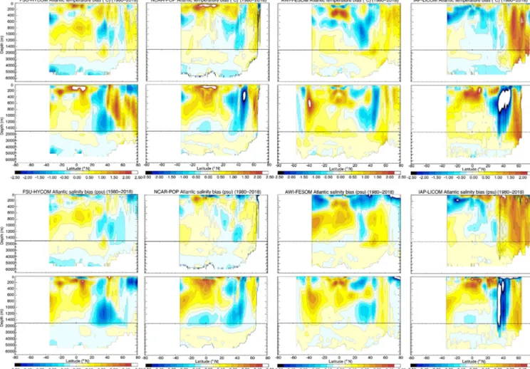
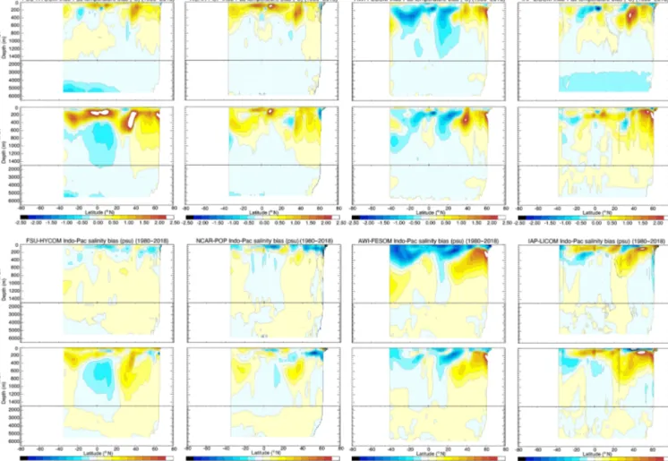
3.3 Temperature and salinity bias (depth vs. time) by ocean basin

Figures 7, 8, and 9 show the time evolutions of the horizontal mean depth profiles of temperature and salinity for the At- lantic, Pacific, and Indian Ocean, respectively. The color bar is the same in all figures, including Fig. 6 (global), therefore allowing for a qualitative estimate of where the drift is most significant. To a large extent, the time evolution in each of the major ocean basins mimics that of the global but with some significant differences. For the Atlantic Ocean (Fig. 7), there is a surface freshening in the upper 100 to 200 m as resolution is increased in FSU-HYCOM, NCAR- POP, and AWI-FESOM. IAP-LICOM, on the other hand, be- comes more saline and warmer in the upper 100 m. The latter is accompanied by a large freshening and cooling below 100 m to approximately 600 m. Overall, the drift is smaller

(10)

Figure 4.Time evolution of global temperature (^◦C) and salinity (psu) change (relative to initial conditions) for all experiments (depth- integrated, upper 700 m, upper 2000 m).

in the Pacific for most models, with a freshening in the upper ocean for all models as resolution is increased. The exception is again IAP-LICOM, which shows a significant increase in salinity in the upper 200 m, and this could be a consequence of the fact that there is no zero normalization of the surface- restoring salt flux. The temperature bias in the Pacific Ocean is similar to that of the global ocean. In the Indian Ocean (Fig. 9), FSU-HYCOM and NCAR-POP exhibit larger biases than AWI-FESOM and IAP-LICOM, but those biases are smaller at the higher resolution.

3.4 Mean temperature and salinity bias

The drift plots from Sect. 3.2 and 3.3 indicate that temperature and salinity bias structures are well-established within the first 2 decades of the spin-up so that time averages com-

puted over the latter decades of the simulations should pro- vide a reasonable estimate of the stationary biases character- izing each model. Figure 10 shows latitude–longitude maps of surface temperature and salinity differences computed over the 1980–2018 time period with respect to WOA18. All models exhibit reductions in sea surface temperature (SST) bias as resolution is increased. The largest bias reductions are seen in the Southern Ocean, in the Agulhas retroflection region, and along the Gulf Stream extension in the North At- lantic. All these changes are presumably primarily related to an improved representation of the pathways of strong surface currents in those regions, which could result not only from differences between resolved and parameterized eddies but also from differences in resolved bathymetry. SST bias in eastern boundary upwelling regions has been shown to

(11)

Figure 5.Time evolution of global temperature (^◦C) and salinity (psu) change (relative to the year 2018) for all experiments and the World Ocean Atlas (WOA18) (depth-integrated, upper 700 m, upper 2000 m).

be strongly sensitive to atmospheric forcing resolution (Tsu- jino et al., 2020), somewhat sensitive to the regridding tech- nique used for near-surface winds (Small et al., 2015), and also slightly sensitive to ocean resolution for seasonal means (Kurian et al., 2020). However, Fig. 10 shows a minimal change in annual mean SST bias in the upwelling zones off the west coasts of Namibia, Peru, and North America. In ad- dition to the Gulf Stream, all models exhibit some degree of bias reduction in the Brazil–Malvinas Confluence zone at high resolution, but no such systematic improvement is evident in the Kuroshio–Oyashio extension region. Sea surface salinity bias is generally reduced globally in the high- resolution simulations, with the exception again being AWI- FESOM, which exhibits a more pronounced negative salinity bias in line with the enhanced near-surface salinity drift at high resolution in that model (see Figs. 6–9). The SSS bias

in the Arctic results from the differences in salinity between WOA18 and the climatologies used in the salinity restoring (GDEM4, WOA13, or PHC3.0; see Sect. 2 for details).

The vertical structure of mean temperature and salinity bias is displayed as zonal averages across the different ocean basins in Figs. 11–13. This reveals that the near- surface global drift toward warming seen in FSU-HYCOM and NCAR-POP is partly related to a degradation of the tropical thermocline in all basins. One hypothesis is that the thermocline bias is related to the representation of vertical eddy heat flux (Griffies et al., 2015), which tends to be stronger and more realistic in high-resolution simulations (see Fig. 5).

In FSU-HYCOM, higher resolution improves the situation, while in NCAR-POP, the tropical thermocline temperature bias actually gets worse with resolution. The degradation in thermocline bias in the POP high-resolution version could

(12)

Figure 6.Time evolution of global temperature (^◦C) and salinity (psu) change (relative to initial conditions) as a function of depth for all experiments.

Figure 7.Time evolution of Atlantic Ocean temperature (^◦C) and salinity (psu) change (relative to initial conditions) as a function of depth for all experiments.

also be due to missing submesoscale physics, which are parameterized in the low-resolution configuration but absent in the high-resolution configuration. In both FSU-HYCOM and NCAR-POP, and to some extent IAP-LICOM, large extrat- ropical and polar temperature biases associated with intermediate and deep waters decrease with enhanced resolution. In AWI-FESOM, both high- and low-latitude biases get worse.

It turns out that the relatively low near-surface temperature drift seen in AWI-FESOM (Figs. 6–9) is related to large,

but largely compensating, anomalies of opposite sign at each depth level. Cold–warm anomalies that develop in the trop- ics and at high latitudes in that model at both resolutions tend to disappear in global or basin-wide means. Such a compen- sation does not occur for salinity, which is too fresh in the thermocline and too saline in deeper intermediate waters in AWI-FESOM, a characteristic that gets worse as resolution is increased. IAP-LICOM exhibits some large changes in the sign and structure of zonal mean bias as resolution changes,

(13)

Figure 8.Time evolution of Pacific Ocean temperature (^◦C) and salinity (psu) change (relative to initial conditions) as a function of depth for all experiments.

Figure 9.Time evolution of Indian Ocean temperature (^◦C) and salinity (psu) change (relative to initial conditions) as a function of depth for all experiments.

but as with AWI-FESOM, it does not lend strong support to the hypothesis that model temperature and salinity bias can be reduced by increasing model horizontal resolution. As already mentioned, the NCAR-POP model exhibits improved representation of high-latitude intermediate and deep waters, but degraded representation of the tropical thermocline, as resolution is enhanced. FSU-HYCOM is the only model that shows a nearly ubiquitous reduction in temperature and salin-

ity bias in all ocean basins in the high-resolution version;

for the other models, greatly enhanced horizontal resolution does not deliver unambiguous bias improvement in all regions. This is a rather unexpected result.

(14)

Figure 10.Modeled surface temperature (^◦C) and salinity (psu) difference from WOA18 over the 1980–2018 time period.

3.5 Northern and Southern Hemisphere sea ice volume and extent

Due to observational constraints, sea ice is often quantified and monitored by passive microwave satellites in terms of sea ice extent (SIE), defined as the sum of all grid areas with 15 % or higher sea ice concentration. Figure 14a–b dis- play the modeled annual mean Northern and Southern Hemi- sphere sea ice extent for all simulations and include comparisons to the latest observations from the National Snow and Ice Data Center (NSIDC) (Fetterer et al., 2017). Sim- ilar to the observations of the 5th and 6th CMIPs (Stroeve et al., 2012; Notz et al., 2020; Shu et al., 2020), the multi- model mean is representative of the passive microwave mean SIE from 1978 to 2018, with large inter-model differences.

All models show a clear decline in SIE in the Northern Hemisphere and weaker trends in the Southern Hemisphere.

Because observed sea ice extent is highly correlated with near-surface air temperature (e.g., Olonscheck et al., 2019), the consistency of the temporal variability between different simulations and observations suggests that this consistency is driven by a realistic JRA55-do forcing. In general, in both hemispheres, an increase in resolution reduces SIE bias, with the exception of IAP-LICOM.

Sea ice volume (SIV) is a second independent measure of sea ice simulation performance that is representative of sea

ice state, determined by the thermodynamical, optical, and dynamical properties of the ice itself, and the sensitivity of modeled SIV to model formulation is insightful for under- standing the physical realism of the sea ice schemes. The modeled time evolution of annual mean Northern and South- ern Hemisphere SIV is displayed in Fig. 14c and d. Rela- tive to SIE, there is significant inter-model spread in SIV.

With the exception of IAP-LICOM, all simulations exhibit a continuous decline in Northern Hemisphere sea ice volume during the satellite era, with trends similar to that of PIOMAS (Schweiger et al., 2011). Changes to SIV also do not appear to be consistent among the models when moving from low to high resolution: it increases for FSU-HYCOM and IAP-LICOM and decreases for NCAR-POP and AWI- FESOM. IAP-LICOM is a clear outlier in both hemispheres, which points to issues in the numerical implementation of its sea ice code at higher resolutions: sea ice thickness on average increases as the resolution is increased despite de- clining SIE. The IAP-LICOM sea ice model has only ther- modynamic processes, and the absence of dynamic sea ice may lead to an excessive accumulation of volume.

3.6 Meridional overturning circulation

The Atlantic meridional overturning circulation (AMOC) is often quantified by a meridional overturning streamfunction

(15)

Figure 11.Global zonal temperature (^◦C) and salinity (psu) difference with the climatology used to initialize the model.

with respect to depth, ψ_z at each latitude, defined as the meridional transport (Sv) across the basin above a constant depthz:

ψ_z(yz)=

0

Z Z

z

v (x⁰, y, z⁰, t )dz⁰dx⁰,

wherevis the 4-D meridional velocity, the overbar denotes a time average (here annual mean), and thex integration cov- ers the entire span of the Atlantic basin. The magnitude of the AMOC, or the AMOC transport, is then defined as the maximum of the streamfunctionψzwith respect toz, representing the total northward transport above the overturning depth (approximately 1000 m in the Atlantic Ocean). This important measure of the AMOC is quantified and monitored by the RAPID moorings near 26.5^◦N (e.g., Smeed et al., 2018).

The modeled annual mean AMOC transport across 26.5^◦N from 1958 to 2018 is displayed in Fig. 15a, along with the RAPID results (2005–2017) for reference. The vertical distribution of the time mean zonal streamfunction in the Atlantic Ocean is shown later in Fig. 26. For the four models, the high-resolution simulations have a higher AMOC

transport than their low-resolution counterparts: the mean AMOC transport in 2004–2018 is 7.8–14.9 Sv in the four low-resolution simulations versus 14.0–19.8 Sv in the four high-resolution simulations (17.2±1.5 Sv as observed by RAPID; e.g., Smeed et al., 2018). However, there is not an obvious difference in the AMOC sensitivity to forcing or in the trend between the low- and high-resolution experiments. The simulated time evolution of the AMOC transports at this latitude depends on the model, its parameterizations, resolution, and the number of spin-up cycles (Dan- abasoglu et al., 2016). Despite the fact that the simulations were only integrated over one JRA55-do cycle (1958–2018), all four low-resolution models show a similar multi-decadal variability, with a transport decrease from 1958 to the late 1970s, an increase from the late 1970s to late 1990s, and a decrease again thereafter. This multi-decadal variability is also present in the CORE-II simulations (Danabasoglu et al., 2016; Xu et al., 2019). In the high-resolution simulations, FSU-HYCOM, NCAR-POP, and AWI-FESOM exhibit a similar multi-decadal variability (of low transports in the late 1970s and high transports in the early 1990s) as seen in previous basin-scale simulations (e.g., Böning et al.,

(16)

Figure 12.Atlantic zonal temperature (^◦C) and salinity (psu) difference with the climatology used to initialize the model.

2006; Xu et al., 2013). The decline in the AMOC transport from the early 1990s to 2000s may be a consequence of the warming and reduced deep convection in the western subpolar North Atlantic that has been documented quite exten- sively (e.g., Häkkinen and Rhines, 2004; Yashayaev, 2007).

The high-resolution AWI-FESOM has a strong AMOC de- creasing trend (of 4–5 Sv) initially during the first 20 years and then has a time evolution of the AMOC that is very similar to that of FSU-HYCOM and NCAR-POP. The high- resolution IAP-LICOM shows an increasing AMOC transport from 1958 to the early 1990s (by 10 Sv) and a decrease thereafter (by 5 Sv), which is quite different from the other three models, but it does appear to capture the observed increase over the last few years.

AMOC transport in the South Atlantic Ocean has been quantified near 34^◦S using several observational techniques including an expendable bathythermograph (XBT), Argo profiles, and moored current meter arrays in the western and eastern boundaries (Baringer and Garzoli, 2007; Dong et al., 2009, 2014, 2015; Garzoli et al., 2013; Goes et al., 2015; Meinen et al., 2013, 2018); these observations yield a time mean AMOC transport of about 14–20 Sv (see Xu et

al., 2020a, for an in-depth discussion of circulation in the South Atlantic Ocean). The modeled temporal evolution of the AMOC transports at this latitude is overall similar to that at 26.5^◦N in the North Atlantic (Fig. 15a, b). The range of the modeled time mean AMOC transport at 34^◦S in the high-resolution simulations, from 14.7 Sv in FSU-HYCOM to 20.1 Sv in IAP-LICOM, is about the same as the observational range mentioned above.

The Antarctic Bottom Water (AABW) cell of the global overturning circulation (Talley, 2013) can be visualized as a streamfunction similar to Eq. (1), except that the zonal integration now spans across the full longitude circle. The transport associated with this cell is defined as the minimum of the streamfunction that is typically found near 3500 m (Lump- kin and Speer, 2007) and is a measure of the northward flow of the near-bottom water (AABW and/or Circumpolar Deep Water, CDW) from the Southern Ocean into the Atlantic, Pacific, and Indian Ocean that eventually upwells and re- turns southward at a shallower depth. Several observational estimates are provided based on hydrographic sections near 32^◦S, but the uncertainty remains quite high (29±7.6 Sv in Talley, 2013). Figure 15c displays the modeled transport at

(17)

Figure 13.Indo-Pacific zonal temperature (^◦C) and salinity (psu) difference with the climatology used to initialize the model.

34^◦S. The low-resolution simulations show a consistently lower transport, with the mean transport value for 2004–

2018 ranging from 7.4 Sv in IAP-LICOM to 15.3 Sv in FSU- HYCOM. The low transport in IAP-LICOM is due to a long- term downward trend in this simulation: from 20 Sv in the early 1960 to 5 Sv in the late 2010s. The other three models, especially FSU-HYCOM, exhibit relatively stable transports in the last 30 years (of the integration). The high-resolution simulations show a much wider range, with time mean transports (2004–2018) ranging from 11.7 Sv in IAP-LICOM to 26.5 Sv in AWI-FESOM. The time evolution of the 34^◦S transports in the high-resolution simulations typically shows an increase in the early stage of the integration followed by a gradual decrease afterward. But the timescale of the increase and decrease periods varies significantly between models. As a result, the transport is relatively stable in IAP-LICOM and AWI-FESOM for the last 30 years of the integration but con- tinues to decrease slowly in NCAR-POP and FSU-HYCOM.

Interestingly, despite the large difference in time mean transports, all four high-resolution models exhibit a similar interannual variability at this latitude for the last 30 years of the integration.

3.7 Drake Passage and Indonesian Throughflow transports

The Antarctic Circumpolar Current (ACC) is a strong oceanic current that flows eastward around Antarctica. It con- nects the Pacific, Atlantic, and Indian Ocean to its north and is the primary means of inter-basin exchange, enabling a truly global overturning circulation (e.g., Gordon, 1986;

Schmitz, 1996; Talley, 2013). Accurate knowledge of ACC transport is fundamental to understand its influence on global circulation. Substantial observational efforts have been made toward quantifying ACC transport, especially in the Drake Passage, where the ACC is constricted between the Antarc- tica and the southern tip of South America. The major observations include (1) the International Southern Ocean Stud- ies (ISOS) program in the late 1970s and early 1980s (Whit- worth, 1983; Whitworth and Peterson, 1985), (2) the repeat hydrographic sections along the World Ocean Circulation Experiment (WOCE) line SR1b (e.g., Cunningham et al., 2003), (3) the repeat shipboard acoustic Doppler current pro- filer (ADCP) surveys that directly measure the current in the top 1000 m of the water column (Firing et al., 2011), (4) the