On the assimilation of absolute geodetic dynamic topography in a global ocean model: impact on the deep ocean state

(1)

https://doi.org/10.1007/s00190-018-1151-1 O R I G I N A L A R T I C L E

On the assimilation of absolute geodetic dynamic topography in a global ocean model: impact on the deep ocean state

Alexey Androsov^1,2 ·Lars Nerger¹·Reiner Schnur³·Jens Schröter¹·Alberta Albertella⁴·Reiner Rummel⁵· Roman Savcenko⁶·Wolfgang Bosch⁶·Sergey Skachko⁷·Sergey Danilov¹

Received: 13 November 2017 / Accepted: 25 April 2018

Abstract

General ocean circulation models are not perfect. Forced with observed atmospheric fluxes they gradually drift away from measured distributions of temperature and salinity. We suggest data assimilation of absolute dynamical ocean topography (DOT) observed from space geodetic missions as an option to reduce these differences. Sea surface information of DOT is transferred into the deep ocean by defining the analysed ocean state as a weighted average of an ensemble of fully consistent model solutions using an error-subspace ensemble Kalman filter technique. Success of the technique is demonstrated by assimilation into a global configuration of the ocean circulation model FESOM over 1 year. The dynamic ocean topography data are obtained from a combination of multi-satellite altimetry and geoid measurements. The assimilation result is assessed using independent temperature and salinity analysis derived from profiling buoys of the AGRO float data set. The largest impact of the assimilation occurs at the first few analysis steps where both the model ocean topography and the steric height (i.e. temperature and salinity) are improved. The continued data assimilation over 1 year further improves the model state gradually. Deep ocean fields quickly adjust in a sustained manner: A model forecast initialized from the model state estimated by the data assimilation after only 1 month shows that improvements induced by the data assimilation remain in the model state for a long time. Even after 11 months, the modelled ocean topography and temperature fields show smaller errors than the model forecast without any data assimilation.

Keywords Dynamic ocean topography · Data assimilation · Ensemble Kalman filter · ESTKF · Geoid · Multi-satellite altimetry

1 Introduction

A major task in oceanography is the determination of currents and associated transports of mass and heat. Velocities

B

Alexey Androsov alexey.androsov@awi.de

1 Alfred Wegener Institute Helmholtz Center for Polar and Marine Research, Am Handelshafen 12, Bremerhaven 27568, Germany

2 Shirshov Institute of Oceanology, Moscow, Russia

3 O.A.Sys GmbH, Hamburg, Germany

4 Politecnico di Milano, Milan, Italy

5 IAPG, TU Munich, Munich, Germany

6 DGFI-TUM, Munich, Germany

7 Meteorological Research Division, Environment and Climatic Change Canada, Dorval, Canada

are difficult to measure directly. However, there is an elegant two-step procedure for their estimation which involves information derived from geodesy. First, using the geostrophic and hydrostatic relationships, the “thermal wind” equations can be derived (Defant1941; Stommel1956). They allow the cal- culation of the vertical velocity shear simply from observed fields of temperature and salinity alone. Vertical integration then yields velocities. The problem has now been reduced to the determination of the remaining integration constant which varies locally. For this second step, two solutions are available, (a) knowledge about the (full) velocity at some depth or (b)—equivalently—a “geostrophic surface velocity” derived from the slope of the sea surface referenced to the geoid.

Making an absolute geodetic surface useful for oceanography has a long tradition. Generations of oceanographers have been searching for a highly accurate reference surface, that can be used to convert relative to absolute oceanic veloc-

(2)

ities and transports (Defant1941). The concept of a “level of no motion” (Stommel1956) is only a convenient approximation in this context assuming the velocity becomes zero at this level. However, it is relatively inaccurate and cannot be applied in areas such as the Southern Ocean. Alternatively

“baroclinic transports” relative to zero bottom velocity have been used (Rintoul and Sokolov2001). Other approaches used data assimilation and inverse modelling to determine absolute velocities (e.g. Wunsch1978).

The concept of using geodetic information simultaneously with oceanic data in a joint estimation process has been introduced decades ago (Wunsch and Gaposchkin1980). It has formed a basis for a long and successful series of satellite oceanographic and geodetic space missions. At the lifetime of the SEASAT and GEOSAT satellite missions, the marine geoid was uncertain to such an extent that only temporal changes were used for oceanic applications. For example, a collinear analysis technique producing sea surface anomalies relative to an unknown or undetermined mean was applied by Cheney and Marsh (1981). Indeed, the primary mission of GEOSAT was to approximate the marine geoidNby measuring a mean altimetric sea surface height (SSH) and correcting it for steric height referenced to a deep level (Douglas and Cheney1990).

The difference between SSH and N is the deviation of the real ocean surface from the geoid, denoted η. It is a characteristic property related to ocean dynamics similar to surface pressure for the atmosphere. Frequently, the difference is called dynamic ocean topography (DOT), averaging it provides the mean dynamic topography (MDT). Although oceanographers conventionally call this quantity differently it is now well understood in the space oceanographic com- munity. The time-varying difference between DOT and MDT is denoted sea-level anomaly (SLA).

The joint estimation ofNand SSH is attractive as the accuracy of gravity and ocean information differs in the spectral domain. The geoid is best known at very long wavelengths with rapid error growth towards shorter wavelengths (blue spectrum). In contrast, the ocean measurements are mostly accurate on small scales and accumulate error on longer scales (red spectrum), see e.g. Rio and Hernandez (2004).

Thus, the combination can result in smaller errors in the shorter and longer wavelengths.

For a long time, it was difficult or even impossible to use the DOT for ocean studies to derive unmeasured quantities, e.g. by data assimilation and inverse modelling (Verron 1992). The difficulty arose from the fact that N was quite uncertain such that only the SLA was representative. One approach to handle DOT data was to replace the mean of the time-dependent DOT by one derived from an ocean model or from an in situ ocean data analysis (Stammer1997). A different approach was to constrain the SLA separately from the mean MDT (Wenzel et al.2001; Stammer et al.2002).

With the first observations from the low earth orbiting CHAMP satellite, the situation changed significantly. The CHAMP geoid (Reigber et al.2002) was sufficiently accurate to subtract it from measurements by altimetric satellites (TOPEX/Poseidon, ERS1/2, JASON), see e.g. Seufer et al.

(2003).

However, the issue of geoid errors on smaller scales remained until the GRACE (Gravity Recovery and Climate Experiment) geoid became available. First studies by Birol et al. (2004, 2005) show the impact of using a geoid of much better resolution instead of a mean dynamic topography MDT. Also they consider the issue of geoid error and resolution as they were limited to a spherical harmonic cut-off degree ofL=60. Stammer et al. (2007) continue their earlier work and constrain the time mean model surface by altimetry minus the GRACE (GGM01c)geoid. Anomalies are con- strained separately. The authors find little impact on the solution and discuss sensitivities as well as insufficient accuracy in the Southern Ocean. A more recent work by Haines et al. (2011) reviews the current research status in using geoid data derived from GRACE to constrain modern ocean general circulation models (OGCMs). The authors also discuss the future prospects of using an improved geoid from the GOCE mission. The need for an even higher-resolution GOCE (Gravity and steady-state Ocean Circulation Explorer) geoid for ocean studies had been pointed out by e.g. LeGrand and Minster (1999); Schröter et al. (2002) and many others. LeGrand (2001) demonstrates how an accurate marine geoid could be used to determine oceanic transports of heat and mass with unprecedented precision.

With the success of the GOCE mission, there are accurate satellite products of DOT that can be assimilated for estimating the ocean state (Rummel1999; Haines et al.2011; Rio et al.2014; Carrere et al.2016; Pail2015). In this study, we focus on the deep ocean and show the current achievements in assimilating such combined product using the finite-element sea-ice ocean model (FESOM, Wang et al.2014). Indeed, we can support findings by Stammer et al. (2007) about the accuracy and about deficiencies in the Southern Ocean. In our present study, we are able to use a DOT with a spherical harmonic cut-off degree of 200 and observe the biggest improvements in the Southern Ocean.

Oceanic transports based on measured hydrography and the slope of the DOT (i.e.) surface geostrophic velocities are uncertain to some extent. In the deep ocean, errors of only 5 cm in DOT lead to errors on the order of 20 Sv (1 Sver- drup corresponds to 10⁶m³s⁻¹). Almost all ocean currents transport less volume which demonstrates the necessity for a highly accurate DOT. Furthermore, velocity fields derived from measurements alone do not obey mass conservation.

To make them mass-consistent, it is common to combine the measurements with an ocean model.

(3)

The estimation of absolute dynamic topography within a system based on an ocean model with assimilation of combined geoid and altimetry data is usually performed by one of two data assimilation approaches: an iterative four- dimensional variational (4D-Var) method minimizing a cost function (Talagrand and Courtier1987) measuring the dis- crepancy between observations and the model or a sequential data assimilation scheme based on the ensemble Kalman filter (EnKF Evensen1994). In the case of EnKFs, data are treated when they are available and the system is driven by short-scale model forecasts. The sequential assimilation approach has been applied in several studies like De Mey and Benkiran (2002) and Bertino and Lisaeter (2008). For the assimilation, the Mean MDT and the SLA data are merged to be assimilated together as an absolute signal.

There are three main issues related to the sequential assimilation approach. The first issue is how to take the errors in the MDT correctly into account so that they are distinguished from the SLA errors. Dobricic (2005) assumed that the error in the MDT field is introduced in the assimilation system as a temporally constant and spatially variable observational bias. The author tried to estimate the MDT error from the differences between long-term averages of MDT and the instantaneous MDT field from the previous time step. The chosen method resulted in an improved SSH analysis. Lea et al. (2008) estimated the MDT errors using a Bayesian approach in the combined MDT and SLA assimilation as an observational bias. In our previous studies (Skachko et al.

2008; Janji´c et al.2011, 2012a,b), we decided to not sepa- rate the geoid and altimetry errors, but to rather increase the assumed DOT errors in the data assimilation system.

The second issue of the sequential assimilation concerns the model performance. As previously stated in Skachko et al.

(2008), the predecessor version FEOM (Danilov et al.2004) of the FESOM model showed a significant sea surface level drift away from the observations. This bias prevented the direct assimilation of the satellite DOT product. To correct the model prior for the data assimilation, the idea of adiabatic pressure correction (Sheng et al. 2001; Eden et al. 2004) was applied. Thus, the sea-level drift was associated with the systematic changes in the thermohaline structure. The chosen method removed the model bias only partially and remained thus suboptimal.

Finally, the third issue in the sequential data assimilation is how to adequately redistribute the observational update on the surface into the ocean depth. In Skachko et al. (2008), we had chosen the method by Fukumori et al. (1999) where the temperature and salinity updates follow the first baroclinic mode in the vertical direction. However, such vertical modes deviate from real modes of variability, which are affected by thermal wind and variable bottom topography and are sensitive to the horizontal amplitude of the perturbations. As an alternative approach, Janji´c et al. (2011,2012a,b) directly

utilized the vertical correlations that are estimated from an ensemble of model state realizations in a ensemble-based SEIK filter. These studies are continued here.

To improve the state estimation by assimilating DOT data in the present work, the current model version of FESOM (Wang et al. 2014) is used with an increased resolution compared to the previous studies. In addition, an improved surface forcing derived from CORE-II inter-annual forcing (Large and Yeager2008) is used. Compared to the studies by Janji´c et al. (2011,2012a,b) also a newer ensemble-based Kalman filter, the ESTKF (Nerger et al.2012a), which keeps the ensemble variance better distributed over all ensemble members than the LSEIK filter used by Janji´c et al. (2011), is applied to assimilate the dynamic ocean topography data.

Further differences include a much more accurate geoid model based on the final GOCE product as well as improved along-track altimetry. Finally, we focus on changes in the deep ocean and show how even a short assimilation time can be used to improve modelled ocean fields over a significant period.

The paper is organized as follows. Section 2 describes the ocean circulation model FESOM. The observations are described in Sect.3followed by the description of the data assimilation method in Sect.4. The results of the data assimilation experiments are discussed with a focus on the vertical structure of the changes induced by the data assimilation procedure in Sect.5. The impact of the data assimilation in different depths and at the surface are discussed in the Sect.6.

Section7concludes the paper.

2 Model description

The numerical experiments of this study have been performed with the Finite-Element Sea-ice Ocean Model (FESOM) (Danilov et al.2004; Wang et al.2008, 2014; Timmermann et al.2009). FESOM is a global coupled ocean-sea ice general circulation model built on finite elements. It uses unstruc- tured triangular meshes in the horizontal directions and tetrahedral elements in the volume. The model uses a contin- uous linear representation for the horizontal velocity, surface elevation, temperature and salinity, and solves the standard set of hydrostatic ocean dynamic primitive equations. It uses a finite-element flux-corrected transport algorithm for tracer advection (Löhner et al.1987).

The configuration of FESOM used in this study is the same as used in the CORE-II intercomparison study, see, e.g., Danabasoglu et al. (2014). The important parameters and characteristics of the model can be found there. The main principles of FESOM and examples of its sensitivity to important governing parameters are discussed by Wang et al.

(2014). The model mesh is configured such that the compu- tational North Pole is located on Greenland. The horizontal

(4)

resolution varies from about 100 km in the open ocean to 25 km in the vicinity of Greenland and to around 30–50 km in the equatorial belt. There are 39 z-levels in the vertical direction. The layer thickness is 10 m in the top ten surface layers and then increases monotonically to 250 m.

Vertical mixing is parameterized using the scheme by Pakanowski and Philander (1981) with the background vertical diffusion of 10⁻⁴m²s⁻¹ for momentum and 10⁻⁵ m²s⁻¹ for tracers. To avoid unrealistically shallow mixed layers that might occur in summer, we introduced an additional diffusivity of 0.01 m²s⁻¹ over the surface mixed layer depth defined by the Monin–Obukhov-length (Timmermann and Beckmann2004). The effects of subgrid- scale processes are parameterized using tracer mixing along isopycnals (Redi1982) and the Gent and McWilliams param- eterization (Gent and McWilliams 1990). The model is forced by the CORE-II inter-annual forcing (Large and Yea- ger 2008). The ocean and sea-ice are first spun up for 35 years, beginning from climatological temperature and salinity, before the data assimilation is applied for the year 2004.

As all models that use the Boussinesq approximation, FESOM conserves volume and not mass. Apart from a gain in numerical efficiency, there is a serious reason for this.

Mass conservation would require sufficient knowledge about inflow and outflow of fresh water through the boundaries of the ocean, i.e. precipitation–evaporation, inflow by rivers, ground water and ice streams. These fluxes are quite large and may be estimated. However, while the relative error of these fluxes may be small, the absolute error is so big that it makes the balance uncertain to an equivalent on the order of 10 mm per year. Accordingly, sea-level change cannot be retrieved from model simulations but has to be measured by tide gauges and is a prime target of space altimetric missions.

The model equivalent of the geodetic DOT is the models surface elevation η, which is closely related to DOT.

Oceanographers referenceηto their coordinate system (z) and they definez=0 being identical to the geoid N. Thus, any secular changes inN such as GIA, self gravitation, etc., are not visible to the ocean model. Associated changes in ocean bottom topography are neglected in general circulation models.

Volume conservation implies that notηbut its horizontal gradient is modelled correctly and only the equation

∇η= ∇DOT

holds. As a consequence, we setη+const = DOT and estimate the constant to be 47 cm by fitting the averageηto DOT over the observed area.

3 Observations

The observations that are assimilated are geodetic dynamic ocean topography (DOT) data. They are derived from filtered geoid and altimetry data in form of a filter-corrected difference. We only provide a short overview of the method here, a more detailed description can be found in Albertella et al.

(2012).

Generally, the DOT is estimated as the difference DOT= SSH−Nof the sea surface height SSH monitored by satellite altimetry and the geoid height N, which describes a geopo- tential surface at the sea level. The quantities SSH andNhave different spectral properties so that both need to be filtered in a consistent way (Bingham et al.2008) to compute the difference. In particular, the geoid height N is a satellite-only gravity field as GOCO03S (Mayer-Gürr et al.2012) and is rather smooth. In contrast, the sea surface heights were computed from the altimeter missions ENVISAT, GFO, Jason-1 and TOPEX/Poseidon and contain a rich spectrum of details observed by the satellite altimeters.

The filtering is performed using the approach by Bosch and Savcenko (2010). Here, the instantaneous SSH is filtered along-track and at the locations where they have been observed. This leads to estimates of instantaneous DOT (iDOT) profiles. To ensure that the along-track SSH is filtered in the same way asN, a filter-correction term was computed using the ultra-high resolving gravity field model EGM2008 (Pavlis et al.2012) in spherical harmonics up to degree and order 2160. This filter-correction term accounts for the difference in the instantaneous one-dimensional filtering of the along-track sea surface heights and the two-dimensional filtering of the geoid. The filtering was applied with an isotropic Gauss-type filter as proposed by Jekeli (1981) with a filter length of 69 km, corresponding approximately to spherical harmonic degreeL =210. For the present paper, the full data set has been evaluated for nearly all sea surface height profiles observed by altimeter satellites operated between 1993 and 2011. A comprehensive cross-calibration of the multi- mission altimeter scenario has been performed in advance (Bosch et al.2014). For this, a 10-day sampling was used such that all iDOT profiles observed within the 10-day intervals were first edited for spurious profiles, then averaged to a global grid with 30spacing and subsequently interpolated to the nodes of the model grid.

4 Data assimilation

4.1 Ensemble filter method

The data assimilation is performed using the error-subspace transform Kalman filter (ESTKF, Nerger et al.2012b) with observation localization (see Nerger et al.2012a). The filter

(5)

algorithm is provided in the Appendix. Here, we present a short overview of the assimilation concept.

The ESTKF is an ensemble square root Kalman filter that assimilates the observational data sequentially in time. For this, an ensemble of model states is used to represent the state estimate and its uncertainty. A forecast ensemble is computed by integrating all ensemble members with the FESOM until the timetk when observations are assimilated. At this time, the ensemble mean state represents the forecast state estimate, while the uncertainty is estimated by the covariance matrix sampled by the forecast ensemble.

At the observation time, an analysis step is computed that incorporates the information from the observations into the model state ensemble. The analysis is computed locally for each water column of the model grid considering only observations within a specified influence radiusl. In addition, the observations are weighted according to their horizontal distance from the water column using a correlation function with compact support. This function is the 5th-order piece- wise rational function of Gaspari and Cohn (1999) whose shape is similar to a Gaussian function. The weighting function is isotropic and decreases monotonically with distance depending on the correlation length scalel/2. The function is positive only for distances that are less thanl and zero otherwise.

The localized ESTKF is implemented in the parallel data assimilation framework (PDAF, Nerger and Hiller 2013, http://pdaf.awi.de). FESOM is coupled to PDAF into a single parallel programme that computes both the ensemble forecasts as well as the analysis step.

4.2 Configuration of assimilation system

The assimilation experiment is performed over the full year 2004. Observations are assimilated at each 10th day. An ensemble of 32 members is used. A preliminary sensitivity study was performed to tune the influence radius for the localization showing that a radius of 580 km provided the smallest Observation-minus-Forecast (OmF) errors. Before each analysis step, a covariance inflation is applied by apply- ing a so-called forgetting factor which increases the spread of the forecast ensemble by 11.8% to stabilize the data assimilation process.

The state vector includes the two-dimensionalηfield as well as the three-dimensional fields of temperature, salinity, and the three components of the velocity. In addition, the variables of the sea-ice model are included.

The ensemble for the assimilation is initialized by combining an initial state estimate with an estimate of the uncertainty. The ensemble mean, representing the initial state estimate, was chosen to be the state at January 1, 2004, from the spin-up run over 35 years initialized from climatology and using the CORE-II surface forcing. The ensemble per-

turbations prescribe the uncertainty of the state estimate.

They have been computed using second-order exact sampling (Pham2001) from each tenth day of the trajectory of the reference run during the year 2004. The resulting ensemble spread was reduced by a factor 0.3 so that initial variance estimate of the ensemble was close to the root-mean-square difference between the initial state estimate and the observations.

To account for the mean difference between the observations and the modelled a constant of 47 cm was added to the model values. For the data assimilation an observation error has to be specified, which represents a combined standard deviation of the observational and modelling (representativeness) errors. Pail (2015) reports geoid uncertainties on the 2–3 cm level, Rio et al. (2014) demonstrate an accuracy of the MDT of 2–3 cm for the Mediterranean. However we deal with the full, time-dependent DOT. Sakov et al. (2012) assume an observational error of 3–4 cm. Since the DOT data does not include a specification of observation errors, we assume a constant of 5 cm (including representativeness error) consistent with our earlier studies (e.g. Janji´c et al. 2012b). We did not attempt to apply a spatially variable representation errors, which might be estimated from sea-level anomalies (see Sakov et al.2012), because of our assimilation of absolute DOT. The observation errors are assumed to be Gaussian and uncorrelated, so that they are represented by a diagonal observation error covariance matrix in the data assimilation.

5 Results

Three experiments have been conducted in this study:

1. FREE: This is a control model simulation over 360 days without data assimilation.

2. ASSIM: In this experiment, the data assimilation system described in Sect.4is applied and the observations are assimilated each 10th day over 360 days. In this experiment, we distinguish between the analysis states directly after the observations at some time are assimilated (referred to as ASSIM-A) and the forecast fields (denoted ASSIM-F), i.e. the model fields obtained at the end of each 10-day model integration of the ensemble states.

3. INFOR: In this experiment, an initialized long forecast is computed from day 30. For this, the model is initialized with the analysis model state (ensemble mean) from the experiment ASSIM on day 30. This experiment is used to assess how the changes in the model states induced by 30 days of data assimilation remain preserved during the following model forecast over 11 months.

(6)

The performance of the experiments is assessed first by using the root-mean-square deviation (RMSD) of the modelled DOT from altimetry observations. A comparison with independent data is performed using Steric Height (SH) at a depth of 2000 m from ARGO-Jamstec (Ishii and Kimoto 2009) data during the simulation year. This comparison is performed with monthly averages for both the model fields and the ARGO observations. Next to the assessment of variance over time, yearly mean differences of modelledηand SH from the observations are examined. A comparison of modelled and measured temperatures at the deepest level of the ARGO data set shows the impact of assimilation at the end of the integration period.

5.1 Dynamic ocean topography

Figure1shows the RMSD of the modelledηfrom the altimetric DOT over the time period from day 10 to day 360.

Without DA, the RMSD varies in the range between 10 and 12 cm during the year in the experiment FREE. In the experiment ASSIM, the DA reduces this deviation to 6.2 cm in the first analysis step at day 10. This deviation is further reduced by the continued DA such that the deviation after the final analysis step is about 3.5 cm. During the 10-day forecasts, the RMSD grows by 2.1 cm at day 10 and later by less than 1 cm per 10 day interval, which is a typical behaviour for sequential data assimilation. The difference between ASSIM-A and ASSIM-F grows during the experiment, but is corrected in each analysis step. The experiment INFOR starts with the analysis of ASSIM at day 30. Thus, it has the same RMSD as ASSIM-A at day 30. Then, the RMSD grows during the 11 months of free model integration. Until day 240, the RMSD from INFOR gets closer to that of FREE. After this day, the growth levels of and the RMSD from INFOR stays between 2.0 and 2.5 cm lower than the RMSD from FREE.

Thus, some information from the changes induced by the three analysis steps in the first month remain in the model state even after 11 months of model integration.

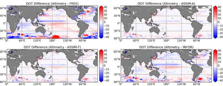
The spatial distribution of the difference between the altimeter data and the modelled ηaveraged over the simulation year is shown in Fig.2. Here, the maps of the mean differences are shown separately for the analyses and the 10-day forecasts. The FREE simulation (top left) shows significant differences from the data of partly more than 40 cm in the Southern Ocean and in the Kuroshio and Gulf Stream regions. In the Tropical Pacific, the model overestimatesη by about 20 cm just north of the equator and underestimates ηabout 10 cm at the equator, which is due to the limited resolution of the model grid.

The data assimilation considerably reduces the η-differences, both in the analysis (ASSIM-A, top right) and the forecast (ASSIM-F, bottom left). All regions with high deviations in the experiment FREE are strongly improved.

Fig. 1 Root-mean-square differences of the modelled DOT from the altimetry observations. The data assimilation results in a strong reduction of the difference, while in the initialized forecast INFOR the RMSD grows slowly

Further improvements are also visible in the Indian Ocean and the North Pacific. The errors are slightly lower in the analysis than the forecast, e.g. in the Tropical Pacific and the Gulf Stream region as is expected from the RMSD discussed before.

As indicated by the RMSD in Fig.1, some of the improvements of the modelledηby the DA remain in the initialized 11-month forecast experiment INFOR. This effect is also visible in the annual mean differences in the lower right panel of Fig.2. Most notably, the differences in the Southern Ocean and the Kuroshio and Golf Stream regions remain significantly lower in INFOR compared to FREE. In the equatorial Pacific and Atlantic, the differences are about 5 cm smaller in INFOR than in the experiment FREE.

The reduction of deviations by the DA is quantified in Fig.3in the form of histograms. The histograms present the probability of differences between altimetry data and model η. They are displayed for the total model domain and sepa- rately for the Tropical Belt (20^◦S to 20^◦N) and the Southern Ocean (south of 40^◦S). The histograms are truncated to the range of±25 cm because larger deviations are very unlikely except for the Southern Ocean as discussed below.

For the whole model domain, the histogram for FREE is rather wide with only about 52% of the surface grid points showing a deviation within the range±5 cm, and 79% of the deviations within the range ±10 cm. The data assimilation results in narrower histograms with a more peaked shape. For ASSIM-F, 85% of the grid points show a deviation within the range of±5 cm, and 96% within the range of±10 cm. These probabilities are ever higher for ASSIM- A with 89% for±5 cm and 97% for±10 cm. Next to the spread of the deviations also the magnitude of the mean

(7)

Fig. 2 Annual mean differences (in cm) between altimetry data and modelledηfor the four cases FREE (upper left); ASSIM-A (upper right); ASSIM- F (bottom left); INFOR (bottom right). The assimilation strongly reduces the differences which slowly grow again in the initialized forecast INFOR

Fig. 3 Histograms ofηdifferences between altimetry and model results: (top) total domain; (bottom right) Tropical Belt; (bottom left) Southern Ocean. The assimilation reduces the deviations in all regions

(8)

Fig. 4 RMSD between altimetry data and modelledη. The assimilation strongly reduces the RMSD. In the initialized forecast INFOR the RMSD are larger, but remain below the case FREE

deviation is reduced from 0.87 cm for FREE, to 0.33 cm in ASSIM-F and 0.24 cm in ASSIM-A. The long forecast in INFOR results in a wider distribution of the deviations compared of ASSIM. However, with 90% of the deviations within the range of±10 cm and 67% within±5 cm, the histogram is still much more narrow than for the case FREE.

For the Tropical Belt the histograms are very similar to those of the total domain. In fact the histograms are a bit more narrow so that the probability of deviations in the range of

±5 cm is about 5% points larger for all four cases. The largest deviations are found in the Southern Ocean. For the case FREE, the histogram is very wide and only about 50% of the deviations are within the range of±10 cm and the mean deviation is 1.08 cm. As visible in Fig.2, the data assimilation results in a strong reduction of the deviations in the Southern Ocean. Accordingly, the histograms for ASSIM- A and ASSIM-F are much more narrow and 93% of the grid points are within the range of±10 cm for ASSIM-F (95% for ASSIM-A). However, the histograms are wider than for the total domain, so that the probability of deviations in the range of±5 cm is lower. The data assimilation also reduced the mean error to 0.45 cm in ASSIM-F and 0.41 cm in ASSIM-A. For the total domain and the Tropical Belt, the long forecast in INFOR results in a wider histogram compared to ASSIM-A and ASSIM-F, but a smaller spread of 79% of the grid points within the range of±10 cm, than in the case FREE.

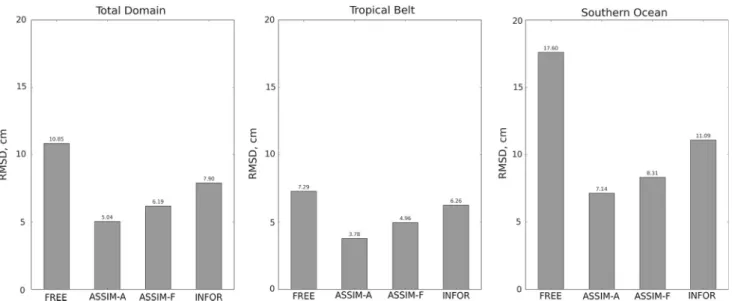
Figure4 summarizes the values of the RMSD over the simulation year, for the whole model domain and separately for the Tropical Belt and the Southern Ocean. For FREE, the averaged RMSD for the total domain is 10.85 cm. This deviation is reduced to about 47% (5.04 cm) in the analysis. In the 10-day forecasts, the averaged RMSD grows to 6.19 cm

(i.e., about 57% of the RMSD from FREE). The RMSD in the Tropical Belt is lower than for the total domain. Here, the case FREE has only an RSTD of 7.29 cm, which is reduced to 3.78 cm in the analysis field of ASSIM-A. The error increase in the 10-day forecasts in the Tropical Belt is 1.18 cm, and hence, a little bit larger than the increase of 1.15 cm in the total domain. The Southern Ocean shows the largest deviations, but also the largest influence of the data assimilation.

For the case FREE, the RMSD is 17.60 cm. The data assimilation reduces the RMSD by 59% to 7.14 cm in the analysis.

The RMSD in the forecast is 1.17 cm larger. For the initialized forecast experiment INFOR, one sees that the increase in RMSD relative to that from FREE is particularly large in the Tropical Belt. Here, the RMSD is 6.26 cm and hence about 85% of that from the case FREE. The increase is particularly low for the Southern Ocean, where the RMSD for INFOR is about 63% of the RMSD from FREE, while for the total domain the RMSD increases to 73% of the value from FREE.

5.2 Steric height

In this section, a further analysis of the results is performed using the independent observations of the steric height from ARGO-Jamstec. While the DOT provides direct information only about the ocean surface, the SH is computed with a reference to 2000 m and is hence giving a vertically integrated information. Because SH depends primarily on depth, the same depth levels must be chosen for a comparison. How- ever model depth and that of the ARGO analysis may differ in shallow areas and only regions with depths of at least 2000 m are considered here. The observational data represents monthly means. To obtain a monthly mean of SH for

(9)

Fig. 5 Root-mean-square differences of the SH from the model from the ARGO-Jamstec data. The continued assimilation keeps the RMS differences below 8 cm, while they grow slowly in the initialized forecast INFOR

the experiment ASSIM, the three analysis steps within each month are averaged. For the experiments FREE and INFOR, daily fields are averaged over each month.

Figure5shows the area average RMSD between the SH from the model and the SH data from ARGO floats over the 12 months of the experiments. For the experiment FREE without data assimilation, the RMSD is between 11.3 and 12.1 cm. The assimilation reduces the RMSD of the SH to about 7.5 cm in the analysis fields. As for the DOT, the 10- day forecasts increase the RMSD. However, for the SH this increase is only of the order of 0.2 cm after 10 days and hence much lower than for the DOT (see Fig.1). The initialized long forecast INFOR also shows a growing RMSD for SH. Similar

to the RMSD of the DOT, the RMSD of SH stabilizes at an asymptotic value at day 210 of the experiment, from which the RMSD of SH is about 9.4 cm, which is about 2.5 cm lower than the RMSD of the experiment FREE. Compared to the DOT, the RMSD of SH in INFOR grows slower. Further, the RMSD shows significantly less variability over time, which is a combined effect of the monthly averages combined with the vertically integrated character of the SH.

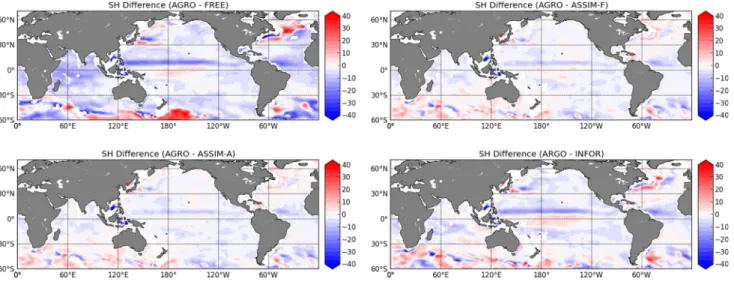
The spatial distributions of the SH difference between ARGO-Jamstec data and the model results are shown in Fig.6 for all the three experiments, where for ASSIM, the analysis and forecast are again shown separately. Regions with ocean depths below 2000 m are shown in white.

As for the DOT, the largest differences of partly more than 35 cm are observed in the Southern Ocean in the experiment FREE. Large differences are also visible in the Kuroshio and Gulf Stream regions and also the equatorial shows deviations similar to those of the DOT. The data assimilation reduces all differences significantly, while in the initialized long forecast case INFOR, the differences grow again.

Figure 7 shows differences in the form of histograms depicting the probability of SH differences analogous to Fig. 3. For the case FREE, the histograms are similar for the total domain and the Tropical belt, while the histogram for the Southern Ocean is much wider. Compared to DOT, the mean deviation is larger for the SH, with 4.85 cm for the total domain, 5.75 cm for the Tropics and 2.54 cm in the Southern Ocean. The data assimilation leads to much stronger peaked histograms such that for the total domain 84% of the grid points show deviations within the range of±5 cm in ASSIM- A, compared to only 41% in FREE. Further, the mean error is reduced to about 2 cm. Also the shape of the histograms

Fig. 6 Annual mean differences in SH (in cm) between ARGO-Jamstec data and modelled SH for the four cases FREE (upper left); ASSIM-A (upper right); ASSIM-F (bottom left); INFOR (bottom right). Regions

with depth below 2000 m are excluded. The differences in the initialized forecast INFOR are larger than in the continued data assimilation, but stay below those of FREE

(10)

Fig. 7 Histograms of SH differences between ARGO data and model results. (top) Total domain; (bottom right) Tropical Belt; (bottom left) Southern Ocean. As for DOT, the differences are significantly reduced by the assimilation

is closer to Gaussian than for FREE. The histograms for the experiment INFOR in the different regions and globally are wider than those for ASSIM-F and ASSIM-A. Striking for the case INFOR is the non-Gaussian shape of the histogram, in particular in the Tropics and the total domain. This indicates that the growth of the deviations in the long forecast is rather linear such that the peaked shape of ASSIM-A is widened without creating significant tails of larger deviations.

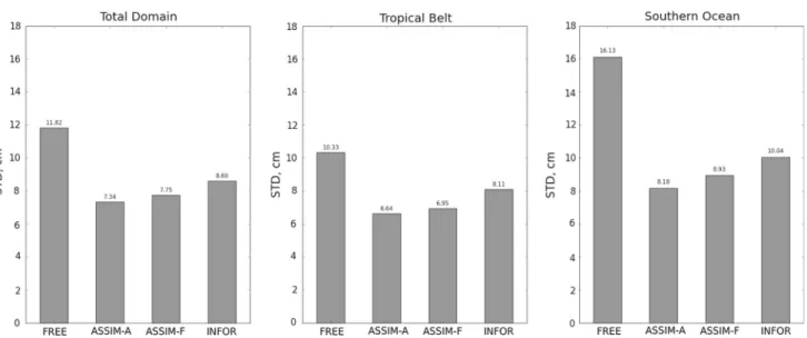
The summary of RMSD values averaged over the simulation year is shown in Fig.8. For the total domain, the assimilation reduced the RMSD of SH to about 62% from 11.82 to 7.34 cm. The RMSD increases only slightly to about 66% in the 10-day forecasts of the case KF. The RMSD of the analysis in ASSIM-A is lower in the Tropical Belt with 6.64 cm and higher with 8.18 cm in the Southern Ocean. In these regions, the assimilation reduces the RMSD to 64% and 51%, respectively. As for the total domain, the 10-day fore-

casts increase the RMSD slightly with the largest increase of about 4% in the Southern Ocean. Overall, the increase in the RMSD for SH is much less than that of DOT (see Fig.4).

In the initialized long forecast case FOR, the RMSD of SH grows further. The growth of the deviation is largest for the Tropical Belt, where the average RMSD is 79% of the RMSD from FREE. For the Southern Ocean, the RMSD is 62% of that from FREE. Hence, while in the Southern Ocean the RMSD grows faster than in the Tropics in the 10-day forecasts, it shows a slower increase on the longer term.

Comparing the effect of the data assimilation on the DOT and the SH, one sees that the correction at each single analysis step is larger for the observed DOT. This causes the larger differences between the ASSIM-A and ASSIM-F in Fig.4 compared to Fig. 8. However, the long persistence of the corrections in the DOT and the strong impact on the SH show that the initially estimated covariance betweenηand the

(11)

Fig. 8 RMSD of SH between ARGO and model results. The error growth in the initialized forecast INFOR is smaller than forη

temperature and salinity fields are sufficiently realistic. This allows the data assimilation method to significantly correct the model state in the multivariate analysis step from the very beginning of the data assimilation experiment with further improvements in the course of the assimilations. Compared to our earlier studies, this successful multivariate assimilation can be explained by the improved model and realistic CORE- II forcing.

6 Impact of the data assimilation at diﬀerent depths and the surface

To assess the impact of the data assimilation at different depths, Fig. 9 shows the percentage of model grid points for which the steric height is changed by the data assimilation by a certain amount over time. Considered at changes of up to 2 cm, between 2 and 5 cm, and more than 5 cm. The panels of the figure show the percentages for different depth regions. For a depth between 0 and 200 m, the upper left panel shows that initially the SH of about 19% of the grid points is changed by more than 5 cm. About 33% of the grid points are changed between 2 and 5 cm, while about 48% of the grid points are only changed up to 2 cm. During the course of the data assimilation experiment (solid lines), the changes grow as is seen from a decrease of the percentage of grid points changed by up to 2 cm and an increase of the percentage of grid points with changes in the bins from 2 to 5 cm and more than 5 cm. At the end of the experiment, about 38% of the grid points are changed up to 2 cm, while 37% are changed between 2 and 5 cm and 25% are change by more than 5 cm.

The influence of the model dynamics is visible from the temporal behaviour of the curves. In particular, the percentage of grid points changed between 2 and 5 cm reaches a maximum

after about 140 days. After about 170 days, the percentage of grid points changed by more than 5 cm shows a minimum of only about 17%, which the percentage of grid points changed by up to 2 cm shows a local maximum. After this time, the percentage of grid points changed by more than 5 cm grows, while the percentage of smaller changes shrinks.

For the depth interval between 200 and 750 m, the initial and final changes are only slightly smaller than for the shallower depth interval. Initially about 51% of the grid points are changed by up to 2 cm, 28% between 2 and 5 cm, and 20%

by more than 5 cm. At the end of the experiment, the changes are larger and about 42% of the grid points are changed by up to 2 cm, 34% between 2 and 5 cm, and 24% by more than 5 cm. Compared to the depth region of up to 200 m, the maximum of changes between 2 and 5 cm are reached later in the experiment around day 270, where also the minimum of grid points changed by up to 2 cm is reached.

Below 750 m depth, the data assimilation still induces notable changes. In the range between 750 and 2000 m depth, about 12% of the grid points are changed by more than 5 cm, which about 24% change between 2 and 5 cm. Also in this depth region the continued data assimilation induced growing changes in the steric height. At the end of the experiment, about 48% of the grid points are changed by more than 2 cm and 16% by even more than 5 cm.

In the largest depth interval, between 2000 m and the ocean bottom, the changes are much smaller. During the course of the experiment only about 1,5% of the grid points are changed by more than 5 cm. Changes between 2 and 5 cm are initially induced for 11% of the grid points. This number grows to about 16% until the end of the experiment.

For the initialized forecast experiment INFOR, Fig. 9 shows that the assimilation-induced changes in the steric height are nearly preserved over the forecast period of

(12)

Fig. 9 Percentage of grid points for which the difference between steric height of the model state without data assimilation from that with data assimilation lies within a specified magnitude. Considered are (solid) the analysis states ASSIM-A of the data assimilation over 1 year and (dashed) the forward run INFOR initialized from the assimilation anal-

ysis mean state after 1 month. The colors show the different magnitudes (red: up to 2 cm, blue: 2–5 cm, green: more than 5 cm). The four panels represent different depth intervals for which the steric heights are computed. Significant changes are visible up to 2000 m depth

11 months. The dashed lines in Fig.9show that for the largest depth, the percentage of grid points changed by more than 5 cm and those changed in between 2 and 5 cm remains nearly constant. The number of grid points changed by up to 2 cm only grows by 1% point. For the depth interval between 750 and 2000 m, the number of grid points changed by more than 5 cm only shrinks from about 12 to 11%, while the number of grid points changed between 2 and 5 cm shrinks from 24 to 20%. For the shallower depth intervals about 48% of the grid points are changed by more than 2 cm. The largest changes of more than 5 cm are observed at the end of the experiment for 18% of the grid points in the depth interval of 200–750 m and about 12% for less than 200 m depth.

Comparing the experiments ASSIM and INFOR, one sees that the continued data assimilation leads to further growing changes compared to the initialized forecast run INFOR.

Nonetheless, the most of the induced changes in the steric

height remain in the model state when the data assimilation is stopped after 1 month and the state estimate at this time is used to initialize a model forward simulation.

Figure 10compares the computed temperature of three experiments with the ARGO data at a depth of 2000 m for the end of the assimilation cycle. At this depth, the free- running model (FREE) is too cold in the Pacific especially in the South. In the Southern Ocean, large areas show a warm bias in the model. The assimilation reduces the errors considerably as is visible for ASSIM-F. The differences between the INFOR integration and ARGO data are very similar to those from ASSIM-F. Essentially only error growth in the Southern Ocean is visible in INFOR. This indicates that most of the error reduction occurs during the first month of assimilations.

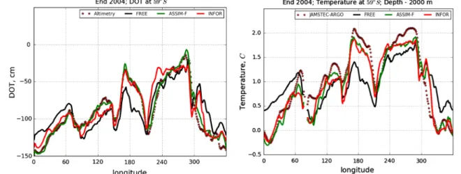
Figure 11 shows DOT and temperature at a depth of 2000 m along the section at a latitude of 59^◦S in the Antarctic Circumpolar Current at the end of the assimilation. The case

(13)

Fig. 10 Temperature fields in December 2004 at a depth of 2000 m.

Upper left panel: Measurements made by the ARGO profiling buoy system; Upper right panel: Difference between ARGO data and the free

model; Bottom left panel: Difference between ARGO data and model after assimilation; Bottom right panel: Difference of ARGO data and the INFOR run. After assimilation the errors are reduced considerably

Fig. 11 Left panel: DOT section along the latitude 59S in the Antarctic Circumpolar Current at the end of the assimilation. Right panel: the corresponding temperature section along the same latitude and the same

time at a depth of 2000 m. The assimilated model is rather close while the INFOR experiment lies between the others, although not everywhere.

By assimilation of DOT also deep temperature fields are corrected

FREE follows the observed DOT only very generally and differs locally by up to 0.4 m. The case ASSIM-F is much closer to the data while the INFOR experiment generally lies between FREE and ASSIM-F, although not everywhere.

As also shown in Fig.10, the assimilation of DOT corrects deep temperature fields. Figure11shows that there is a close relationship between temperature and DOT in this region.

While the observed DOT can be approached fairly closely, the modelled temperature remains too cold in most areas by a few tenths of a degree.

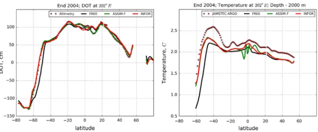
The ocean state at the end of the assimilation year in a south–north section through the deep Pacific Ocean along the longitude 202^◦E is considered in Fig.12. Again both DOT and the temperature at a depth of 2000 m are shown.

Between 50^◦S and 60^◦S the assimilation of DOT data shifts the position of the Antarctic Circumpolar Current by a few 100 km to its correct location. This correction is kept until the end of the year in the INFOR experiment. Further north the case ASSIM is able to follow the observed DOT while INFOR exhibits the same tendency as FREE in underesti- mating DOT south of the equator and overestimating it north of it. Over all, the modelled temperatures have a cold bias. To correct the position of the ACC, the temperature is increased substantially in the Southern Ocean. However, the temperature always stays below the temperature measured by ARGO.

The case INFOR is nearly identical to ASSIM-F over most of the section except in the equatorial region. Here, an inter- esting feature is visible as ASSIM-F compensates missing

(14)

Fig. 12 Left panel: A southnorth DOT section through the deep Pacific Ocean along the longitude 202E and at the end of the assimilation.

Right panel: The corresponding temperature section along the same longitude and the same time at a depth of 2000 m. By assimilation of

DOT the position of the Antarctic Circumpolar Current can be shifted by a few 100 km to its correct location. Modelled temperatures have a cold bias. To correct the position of the ACC, temperature is increased substantially in the Southern Ocean

ocean dynamics by changing temperature and thus the steric height on a short spatial scale.

7 Conclusion

Absolute dynamic sea surface height (DOT) obtained from combining satellite altimetry and geoid data has been assimilated in a global configuration of the finite-element sea-ice ocean model (FESOM). The model was configured with a rather coarse horizontal resolution of about 100 km in the open ocean and finer resolution in the vicinity of Greenland and in the equatorial band. The ocean surface was forced by the realistic CORE-II forcing. The assimilation applied the ensemble-based error-subspace transform Kalman filter (ESTKF) with localization.

The assimilation experiment shows that the assimilation has the largest impact at the first analysis step in which the root-mean-square difference (RMSD) between the modelled DOT and altimetry observations is reduced from about 10.5 to 6.3 cm. Subsequent analysis steps at each 10th day continue to reduce the deviation. However, their impact is only of order of 1–1.5 cm and mainly reduce the deviation-increase resulting from the model forecast of each 10 days so that the RMSD decreases gradually. The assimilation efficiently corrects large deviations of partly more than 40 cm, e.g. in the Southern Ocean and the Gulf Stream and Kuroshio regions.

An assessment of the difference of the steric height (SH) in the model state and data from ARGO-Jamstec shows that the assimilation corrects the model state also in the deep ocean.

As for the modelledη, the largest corrections of SH are at the initial analysis time, while later analysis steps cause smaller

corrections. The smallest deviations for both DOT and SH are found in the Tropical Belt, while the deviations are largest in the Southern Ocean.

A single model forecast over 11 months was initialized from the state estimate after three analysis steps. This forecast shows that part of the improvements induced by assimilating DOT data remain in the model state over the full 11 months.

The deviation from the satellite altimetry data increases gradually for about 6 months. After this time, the deviation shows no trend any more, and even after 11 months, the deviation is about 2.5 cm less than the RMSD in the free model forecast without any data assimilation. The deviation of the SH from ARGO-Jamstec data shows an analogous behaviour.

Analysing the influence of the assimilation in the deeper parts of the ocean, one finds that for SH below 2000 m about 10% of the grid points are influenced between 2 and 5 cm during the first few analysis steps. This value remains about constant for the forecast run initialized after 3 analysis steps.

For the continued assimilation the fraction of grid points influenced between 2 and 5 cm gradually increases to about 17%. In the depth range between 750 and 2000 m, the corrections are larger. About 37% of the grid points are changed by more than 2 cm and 12% by even more than 5 cm at the beginning of the data assimilation. The continued assimilation increases the number of grid points corrected by more than 2 cm to about 48%, while in the 11-month initialized forecast, the fraction is gradually reduced to about 32%.

Overall, the experiments show that with the realistic CORE-II forcing, the model is able to produce realistic dynamics so that the correlations between DOT and temperature and salinity in the ensemble of model states that is used to initialize the data assimilation process are also real-

(15)

istic. This allows the ensemble filter to successfully correct the three-dimensional model fields even in deeper layers.

Assessing the temperature field at a depth of 2000 m at the end of the assimilation a clear improvement is visible due to the assimilation of DOT data. Also for temperature the INFOR experiment keeps the memory of the corrections induced during the first month of assimilation for the rest of the year. These results are very encouraging and possibly helpful when model trends have to be reduced for future applications. However, the assimilation was unable to fully reduce the cold bias of our model at depth. This, however, is not unexpected as ensemble Kalman filters assumed unbiased errors, which is not the case here. Thus more research work, like the addition of a bias-correction scheme, is necessary to this end.

While the assimilation impact is largest at the first analysis step, the continued assimilation has a gradual effect. Using the model state estimate after just three analysis steps shows that the correction are retained in the model state for a long time period. This effect is likely caused by the rather coarse model resolution which induces rather slow dynamics.

The next natural steps for continuing this series of studies would be to first to assimilate ARGO profiles in addition to DOT. However, the ARGO array is coarse with a nominal resolution of 3 by 3^◦. Anyway, we may expect an impact on the large-scale fields and hopefully a reduction in the cold bias of our model. The second natural extension is to increase the model resolution substantially such that eddies and oceanic fronts are realistically represented. Then, one could make use of the full resolution of the geodetic DOT and improve our understanding of ocean dynamics.

Appendix: The error-subspace transform Kalman ﬁlter

The error-subspace transform Kalman filter (ESTKF, Nerger et al. 2012b) combines the information from a forecast ensemble X_k^f of m model states of size n in the columns of this matrix and the observationsykof dimension pat the timetkby the transformation

X^a_k =X_k^f +X_k^fWk (1) of the forecast ensemble into an analysis ensembleX^a_krepre- senting the analysis state estimate and its uncertainty. Here, Wkis a transformation matrix of sizem×m. The matrixX_k^f holds the ensemble mean state in each column. As all com- putations in the analysis refer to the timetk, the time indexk is omitted below.

The ESTKF computes the ensemble transformation matrix Win the error-subspace of dimension m−1 that is repre-

sented by the forecast ensemble. An error-subspace matrix is defined by

L:=X^fT (2)

where the matrixTis a projection matrix of sizem×(m−1) defined by

Tj,i :=

⎧⎪

⎪⎪

⎨

⎪⎪

⎪⎩

1−_m¹ √1¹

m+1 fori = j,j <m

−_m¹ √1¹

m+1 fori = j,j <m

−^√¹_m for j =m.

(3)

A model state vectorx^f and the vector of observationsy are related through the observation operatorHby

y=H

x^f

+ . (4)

The vector of observation errors,, is assumed to be a white Gaussian distributed random process with the observation error covariance matrixR.

For the analysis step, a transform matrix in the error- subspace is defined by

A⁻¹:=ρ(m−1)I+(HX^fT)^TR⁻¹HX^fT. (5) The matrix has size(m−1)×(m−1)andIis the identity matrix. The factorρwith 0< ρ≤1 is called the “forgetting factor” and is used to inflate the forecast error covariance matrix.

The analysis ensemble is given by X^a=X^f +X^f

W+ ˜W

(6) withW:=[w, . . . ,w] and

w:=TA

HX^fT T

R⁻¹

y−Hx^f

, (7) W˜ :=√

m−1TCT^T. (8)

Here,wis vector of sizemthat corrects the ensemble mean, whileW˜ transforms the ensemble perturbations. In Eq. (8), Cis the symmetric square root ofAthat is computed from the eigenvalue decompositionUSV = A⁻¹such thatC = US⁻¹^/²U^T.

For the localized analysis, each vertical water column of the model grid is updated independently by a local analysis step. We denote a water column by the indexσ, i.e. the local sub-state for a water column isx_σ^f. For each local analysis only observations within a horizontal influence radiuslare taken into account so that also observations outside the water columnσare used. A local observation domain is denoted by

(16)

the indexδ. The local observation operatorH_δnow computes an observation vector within the local observation domain from the global model state. With localization, Eq. (1) is applied with an individual matrixWfor each local analysis domain.

Each observation is weighted according to its distance from the water column by the observation localization (Hunt et al.2007). The weight is applied by replacing the inverse observation error covariance matrix in Eqs. (5) and (7) by R˜ =D_δ◦R_δ⁻¹. (9) Here,◦denotes the element-wise matrix product.D_δis the localization weight matrix that is constructed from a correlation function with compact support. The value of the localization function decreases with the distance between the updated water column and the location of the observation until it becomes zero at the specified influence radius. A typical localization function is a 5th-order polynomial with a shape similar to a Gaussian function (Gaspari and Cohn 1999).

An implementation of the local ESTKF, including par- allelization, is implemented in the open-source release of the parallel data assimilation framework (PDAF, Nerger and Hiller2013,http://pdaf.awi.de).

Acknowledgements This study was supported by the Deutsche Forschungs- gemeinschaft (DFG) priority programmes SPP1257 (Massentransporte) and 1788 (Dynamic Earth).

Open Access This article is distributed under the terms of the Creative Commons Attribution 4.0 International License (http://creativecomm ons.org/licenses/by/4.0/), which permits unrestricted use, distribution, and reproduction in any medium, provided you give appropriate credit to the original author(s) and the source, provide a link to the Creative Commons license, and indicate if changes were made.

References

Albertella A, Savcenko R, Janjic T, Rummel R, Bosch W, Schröter J (2012) High resolution dynamic ocean topography in the Southern Ocean from GOCE. Geophys J Int 190:922–930

Bertino L, Lisaeter K (2008) The topaz monitoring and prediction system for the atlantic and arctic oceans. J Oper Oceanogr 1(2):15–18 Bingham RJ, Haines K, Hughes CW (2008) Calculating the ocean’s mean dynamic topography from a mean sea surface and a geoid. J Atmos Ocean Technol 25:1808–1822

Birol F, Brankart JM, Castruccio F, Brassuer P, Verron J (2004) Impact of ocean mean dynamic topography on satellite data assimilation.

Marine Geod 27:59–78

Birol F, Brankart JM, Lemoine JM, Brasseur P, Verron J (2005) Assim- ilation of satellite altimetry referenced to the new GRACE geoid estimate. Geophys Res Lett 32(6):L06601

Bosch W, Dettmering D, Schwatke C (2014) Multi-mission cross- calibration of satellite altimeters: constructing a long-term data record for global and regional sea level change studies. Remote Sens 6:2255–2281

Bosch W, Savcenko R (2010) On estimating the dynamic ocean topography—a profile approach. In: Mertikas In (ed) Gravity, Geoid and Earth Observation, IAG Symposia, vol 135. Springer, Berlin, pp 263–269

Carrere L, Faugere Y, Ablain M (2016) Major improvement of altimetry sea level estimations using pressure-derived corrections based on ERA-Interim atmospheric reanalysis. Ocean Sci. 12:825–842.

https://doi.org/10.5194/os-12-825-2016

Cheney EE, Marsh JG (1981) Seasat altimeter observations of dynamic topography in the gulf stream region. J Geophys Res Oceans 86(C1):473–483

Danabasoglu G, Yeager SG, Bailey D, Behrens E, Bentsen M, Bi D, Biastoch A, Böning C, Bozec A, Canuto VM, Cassou C, Chas- signet E, Coward AC, Danilov S, Diansky N, Drange H, Farneti R, Fernandez E, Fogli PG, Forget G, Fujii Y, Griffies SM, Gusev A, Heimbach P, Howard A, Jung T, Kelley M, Large WG, Leboissetier A, Lu J, Madec G, Marsland SJ, Masina S, Navarra A, Nurser AG, Pirani A, y Mélia DS, Samuels BL, Scheinert M, Sidorenko D, Treguier A-M, Tsujino H, Uotila P, Valcke S, Voldoire A, Wang Q, (2014) North Atlantic simulations in coordinated ocean-ice reference experiments phase II (CORE-II). Part I: mean states. Ocean Model 73:76–107

Danilov S, Kivman G, Schröter J (2004) A finite-element ocean model:

principles and evaluation. Ocean Model 6:125–150

De Mey P, Benkiran M (2002) A multivariate reduced-order opti- mal interpolation method and its application to the Mediterranean basin-scale circulation. In: Pinardi N, Woods J (eds) Ocean fore- casting, conceptual basis and applications. Springer, Berlin, pp 281–305

Defant A (1941) Die absolute Topographie des physikalischen Meeres- niveaus und der Druckflächen, sowie die Wasserbewegungen im Atlantischen Ozean. Wiss Ergebn Dtsch Atlant Exped Meteor 6/2(5):318

Dobricic S (2005) New mean dynamic topography of the mediterranean calculated from assimilation system diagnostics. Geophys Res Lett 32(11):L11606

Douglas BC, Cheney R (1990) Geosat: beginning a new era in satellite oceanography. J Geophys Res Oceans 95(C3):2833–2836 Eden C, Greatbatch R, Böning C (2004) Adiabatically correcting an

eddy-permitting model using large-scale hydrographic data: application to the Gulf Stream and the North Atlantic current. J Phys Oceanogr 34:701–719

Evensen G (1994) Sequential data assimilation with a nonlinear quasi- geostrophic model using Monte Carlo methods to forecast error statistics. J Geophys Res 99(C5):10143–10162

Fukumori I, Raughunath R, Fu L, Chao Y (1999) Assimilation of TOPEX/Poseidon altimeter data into a global ocean circulation model: how good are the results? J Geophys Res 104:25647–25665 Gaspari G, Cohn SE (1999) Construction of correlation functions in

two and three dimensions. Q J R Meteorol Soc 125:723–757 Gent P, McWilliams J (1990) Isopycnal mixing in ocean circulation

models. J Phys Oceanogr 20:150–5

Haines K, Johannessen JA, Knudsen P, Lea D, Rio M-H, Bertino L, Davidson F, Hernandez F (2011) An ocean modelling and assimilation guide to using goce geoid products. Ocean Sci 7(1):151–164 Hunt BR, Kostelich EJ, Szunyogh I (2007) Efficient data assimilation for spatiotemporal chaos: a local ensemble transform Kalman filter.

Physica D 230:112–126

Ishii M, Kimoto M (2009) Reevaluation of historical ocean heat content variations with time-varying XBT and MBT depth bias corrections.

J Oceanogr 65:287–299

Janji´c T, Nerger L, Albertella A, Schröter J, Skachko S (2011) On domain localization in ensemble based Kalman filter algorithms.

Month Weather Rev. 139:2046–2060

Janji´c T, Schröter J, Albertella A, Bosch W, Rummel R, Schwabe J, Scheinert M (2012a) Assimilation of geodetic dynamic ocean