Biome partitioning of the global ocean based on phytoplankton biogeography

(1)

Research Collection

Journal Article

Biome partitioning of the global ocean based on phytoplankton biogeography

Author(s):

Hofmann Elizondo, Urs; Righetti, Damiano; Benedetti, Fabio; Vogt, Meike Publication Date:

2021-06

Permanent Link:

https://doi.org/10.3929/ethz-b-000479179

Originally published in:

Progress in Oceanography 194, http://doi.org/10.1016/j.pocean.2021.102530

Rights / License:

Creative Commons Attribution 4.0 International

This page was generated automatically upon download from the ETH Zurich Research Collection. For more

information please consult the Terms of use.

(2)

Progress in Oceanography 194 (2021) 102530

Available online 24 March 2021

Biome partitioning of the global ocean based on phytoplankton biogeography

Urs Hofmann Elizondo

^*

, Damiano Righetti, Fabio Benedetti, Meike Vogt

Environmental Physics Group, Institute of Biogeochemistry and Pollutant Dynamics, ETH Zürich, Universit¨astrasse 16, 8092 Zürich, Switzerland

A R T I C L E I N F O Keywords:

Biomes Phytoplankton Self-organizing map Indicator species Species network Species distribution models

A B S T R A C T

Biomes are geographical units that can be defined based on biological communities sharing specific environmental and climatic requirements. Contemporary ocean biomes have been constructed based on various ap- proaches. These included the biogeographic patterns of higher trophic level organisms, physical and biogeochemical properties, or bulk biological properties such as chlorophyll-a, but none considered the biogeographic patterns of the first trophic level explicitly, i.e. phytoplankton biogeography. A global description of marine biomes based on phytoplankton and defined in analogy to terrestrial vegetation biomes is still lacking.

A bioregionalization based on phytoplankton appears particularly timely, as phytoplankton have a high sensitivity to climatic changes and fuel marine productivity. Here, we partition the global ocean into biomes by using self-organizing maps and hierarchical clustering, drawing on the biogeographic patterns of 536 phytoplankton species predicted from empirical evidence. Our approach reveals eight different biomes at the seasonal scale, and seven at the annual scale. The biomes host characteristic phytoplankton species compositions, and differ in their prevailing environmental conditions. The largest differences in phytoplankton composition are found between a Pacific equatorial biome and other tropical biomes, and between subtropical and high latitude biomes. The Pacific equatorial biome is characterized by species with narrower ecological niches, the tropical and subtropical biomes by cosmopolitan generalists, and the high latitudes by species with a heterogeneous biogeography. The strongest differences between biomes are found along gradients of temperature and macronutrient availability, associated with latitude. We test whether our biomes can be reproduced based on indicator species, or potential co-occurrence networks of species determined from the predicted species distributions that are wide-spread in some but rare in other biomes. We find that our biomes can be reproduced by the 51 species identified, which together form significant species co-occurrences. This suggests that species co-occurrences, rather than individual indicator species drive oceanic biome partitioning at the first trophic level. Our biome partitioning may be especially useful for comparative analyses on the functional implications of phytoplankton organization, and impacts on zoogeographical partitionings. Furthermore, it provides a framework for predicting large-scale changes in phytoplankton community structure due to anthropogenic climate and environmental change.

1. Introduction

Biomes classify global natural biodiversity, including species as- semblages and countless ecosystem types into geographic realms with distinct life forms, which provide similar ecosystem services. Classically, terrestrial biomes have been delimited by rather sharp transitions in vegetation type driven by global climatic gradients of temperature and precipitation (Bailey, 1998; Townsend et al., 2008). These biomes have emerged from characteristic life-forms and plant functional traits that

represent adaptations to the climatic zones (Ringelberg et al., 2020).

Originally focusing on vegetation (e.g. Clements, 1917; Whittaker, 1970), the biome concept was later expanded to include differences in ecosystem services and functions (e.g. Higgins et al., 2016; Silva de Miranda et al., 2018), with results being compared to terrestrial zoogeographic partitionings (Ficetola et al., 2017; Holt et al., 2012;

Wallace, 1876). Over the past three decades, biomes have been increasingly delineated in the ocean system, yet the biotic and environmental factors used to define such biomes vary strongly between

* Corresponding author.

E-mail addresses: urs.hofmann@usys.ethz.ch (U. Hofmann Elizondo), damiano.righetti@env.ethz.ch (D. Righetti), fabio.benedetti@usys.ethz.ch (F. Benedetti), meike.vogt@env.ethz.ch (M. Vogt).

Contents lists available at ScienceDirect

Progress in Oceanography

journal homepage: www.elsevier.com/locate/pocean

https://doi.org/10.1016/j.pocean.2021.102530

Received 31 January 2020; Received in revised form 15 January 2021; Accepted 15 February 2021

(3)

studies. While some studies relied on environmental and biogeochemical characteristics (Sarmiento et al., 2004; Oliver and Irwin, 2008; Fay and McKinley, 2014; Zhao et al., 2019), others implemented biological criteria. Recent studies have drawn on the taxonomic biogeography of zooplankton and higher trophic level organisms (Reygondeau et al., 2011; Sutton et al., 2017; Costello et al., 2017), both biological and physical factors (Longhurst, 1995; Spalding et al., 2012), or they have contested the applicability of the biome concept to the ocean (van der Spoel, 1994; Ekman, 1953).

Currently, the most widely-used marine classification separates the ocean into 57 provinces using physical properties (temperature, salinity, turbulence), chlorophyll concentration, primary production, and in-situ zooplankton observations (Longhurst, 1995, 2007). In similarity to the terrestrial biomes concept, this partitioning aimed to establish a link between ecosystem structure and function, and strived to characterize the ocean’s carbon budget and its seasonality (Longhurst, 1995). The approach by Longhurst (1995) assumed a bottom-up control of abiotic factors over marine ecosystems structure and species composition, in which physical processes shaped plankton communities via nutrient supply, ambient temperature, and light availability. Similar studies have expanded on Longhurst’s work and objectively distinguish ecoregions from satellite observables such as sea surface temperature, nutrient concentration, and chlorophyll-a concentration (Vichi et al., 2011;

Hardman-Mountford et al., 2008). Nevertheless, the definition of these marine provinces has been debated, given the lack of inclusion of more detailed biogeographic information on taxa, their static nature (e.g.

Vichi et al., 2011; Reygondeau et al., 2013), and given their possible lack of significance for biological communities and ecosystem functions (Vichi et al., 2011).

Marine bioregionalizations based on taxonomic biogeography have often been of regional character (Waters et al., 2010; Kulbicki et al., 2013; Griffiths et al., 2009; Briggs and Bowen, 2011), have focused on individual taxa (e.g. Radiolaria Polycistina; Boltovskoy and Correa, 2016), taxa of coastal and shallow seas (Briggs and Bowen, 2011;

Spalding et al., 2007), or higher trophic level taxa, including top pred- ators such as tuna and billfish (Reygondeau et al., 2011). Although global biodiversity distributions in the ocean have been recently characterized for phytoplankton (Righetti et al., 2019a) as well as zooplankton and marine mammals (Tittensor et al., 2010), Costello et al.

(2017) defined the only generalized, global-scale, multi-taxa marine bioregionalization (Zhao et al., 2019). Costello et al. (2017) partitioned the ocean into 30 marine regions based on the occurrence observations of 65^′000 pelagic and benthic species spanning eleven different phyla (of which 96% are heterotrophic, e.g. Arthropoda, Mollusca, Chordata).

This partitioning resulted in a set of unique ecological provinces with a high degree of species endemicity (Costello et al., 2017). Similar zoogeographic studies in terrestrial and marine systems have suggested that biomes may be strongly dependent on the trophic level addressed and the climatic or evolutionary drivers of individual taxa, within a hierarchically nested structure (Ficetola et al., 2017; Spalding et al., 2012). Hence, Costello’s regionalization of the open ocean may be characteristic for fauna, but does not consider the degree of geographic variability in lower trophic level organisms, such as autotrophs, that inhabit the niche space of the entire surface ocean, with many abundant cosmopolitan species (Brun et al., 2015).

In summary, current ocean partitionings have either been based on environmental, biogeochemical, and bulk biological properties such as chlorophyll-a (e.g. Oliver and Irwin, 2008; Fay and McKinley, 2014;

Vichi et al., 2011; Kavanaugh et al., 2014) or the distribution and biogeographic patterns of higher trophic level organisms (Reygondeau et al., 2011; Costello et al., 2017). However, none of them has considered the biogeographic patterns of the ocean’s main primary producers, the phytoplankton. Partitionings based on environmental and biogeochemical properties (e.g. Longhurst, 2007) have revealed distinct differences in environmental conditions between biomes, but biomes have tended to overlap in their biological bulk properties (e.g. chlorophyll-a

concentration or bacterial and heterotrophic biomass; Vichi et al., 2011). The first zoogeographic partitionings lead to a large number of biologically unique biomes with a high degree of endemicity, yet these biomes are sensitive to specific taxa and trophic levels considered (Costello et al., 2017; Ficetola et al., 2017), and the links between ecosystem structure and ecosystem function have not yet been established.

Owing to the recent increase in global plankton distribution data based on satellites (e.g. Moisan et al., 2017; Navarro et al., 2014;

Bracher et al., 2015; Sathyendranath et al., 2014), research cruises (see e.g. Villar et al., 2018), and global species projections (Righetti et al., 2019a), a classification of the ocean into biomes using phytoplankton biogeography has now become possible. Phytoplankton constitute the basis of marine food-webs (Litchman, 2007), and changes in matter and energy input from phytoplankton communities therefore cascade to- wards higher trophic levels (Voigt et al., 2003; Sarmento et al., 2010).

Phytoplankton have been shown to influence global biogeochemical cycles (e.g. Falkowski, 1998; Bopp et al., 2005; Mor´an et al., 2010;

Litchman et al., 2015; Guidi et al., 2016), and to respond sensitively to environmental change (e.g. Reid et al., 2007; Beaugrand, 2009). Hence, analogous to terrestrial primary producers counterparts, major marine primary producers (Field, 1998) are likely to partition the ocean into geographically constrained and ecologically distinct units with relevance for ecosystem function and global biogeochemical cycling. The wide environmental niches found in phytoplankton (Brun et al., 2015), spanning on average 16^◦C in the surface ocean (Righetti et al., 2019a), suggest that an ocean partitioning based on phytoplankton species distribution will result in a lower number of biomes compared to partitionings based on higher trophic level taxa, with the latter partitionings potentially being nested within phytoplankton-based biomes (Costello et al., 2017). Moreover, differences in phytoplankton composition from one region to another have been shown to reflect seasonal variability of environmental and biogeochemical patterns (Mojica et al., 2015; Righ- etti et al., 2019a). Biomes based on phytoplankton biogeography may integrate top-down and bottom-up factors controlling ecosystem structure and function, since both biotic and abiotic factors have been shown to govern phytoplankton composition (Lima-Mendez et al., 2015; Boyd et al., 2010; Brun et al., 2015; Endo et al., 2018), and phytoplankton species communities display local associations with distinct physico- chemical conditions (Logares et al., 2014; Endo et al., 2018), as well as processes related to global biogeochemical cycling and the biological carbon pump (Guidi et al., 2016).

A major quest associated with the biogeochemical and ecological relevance of marine biomes is their link to specific ecosystem functions (Hattam et al., 2015; Townsend et al., 2018) such as the maintenance of biodiversity, productivity or essential biogeochemical processes (Gam- feldt and Roger, 2017; Manning et al., 2018). To this end, the link between biodiversity, ecosystem structure, or species composition, and essential ecological or biogeochemical functions needs to be investi- gated. At present, it is unclear to what degree planktonic ecosystem functions may be quantified based on the abundance or activity of individual predominant species (Schwartz et al., 2000), species networks (Guidi et al., 2016), or the full spectrum of species diversity (Goebel et al., 2014; Vallina et al., 2014; Cermeno et al., 2013). Phytoplankton ˜ species diversity has been shown to be positively correlated with ecosystem services such as primary productivity (Ptacnik et al., 2008;

Goebel et al., 2014). Primary productivity may be predominantly car- ried out by the most abundant species rather than the full spectrum of diversity (see Schwartz et al., 2000; Cerme˜no et al., 2013), and certain ecosystem functions tend to increase rapidly with increasing species richness and saturate asymptotically at higher richness, (see Schwartz et al., 2000; Goebel et al., 2014; Vallina et al., 2014). While a few dominant species may essentially drive ecosystem processes at any particular snapshot in time (Lyons et al., 2005; Cermeno et al., 2016), a ˜ vast number of rare species present in the plankton (Ser-Giacomi et al., 2018) may stabilize these processes over time, as species may quickly

(4)

assemble and raise to dominance in a variable environment. As a consequence, phytoplankton networks rather than individual dominant species may maintain ecosystem function and services in the ocean, including the biological carbon pump (Strom, 2008; Decelle et al., 2012;

Lima-Mendez et al., 2015; Guidi et al., 2016). Hence, a key task in plankton ecology is to determine ecosystem constituents (e.g. dominant species or species networks) that are essential to ecosystem functions.

Delineating biomes that emerge from these constituents that emerge from the most common and wide-spread species may offer a valid alternative to traditional biomes and become essential tools for global marine ecosystem monitoring and management.

In this study, we partitioned the open ocean into biomes using newly available, monthly biogeographic patterns of 536 phytoplankton species (Righetti et al., 2019b), and self-organizing maps (Fendereski et al., 2014; Kavanaugh et al., 2014). Our partitioning of the ocean into biomes allowed us to test the hypotheses that (i) the open ocean can be partitioned into ecologically relevant biomes based on biogeographic patterns of phytoplankton species, (ii) biome boundaries are dynamic in nature and vary throughout the year, (iii) biomes are characterized by distinct phytoplankton species compositions, and (iv) by characteristic indicator species or phytoplankton species co-occurrence networks, and (v) biomes differ in their prevailing environmental and biogeochemical conditions, as well as in their productivity.

2. Data and methods

2.1. Phytoplankton species occurrence projections

Biomes were constructed based on monthly distribution maps of species’ presence derived from statistical species distribution model (SDM) ensembles developed by Righetti et al. (2019a). These models were adapted to the relatively sparse data available for many species and addressed the spatio-temporal bias present in sampling density through pseudo-absence selection techniques (i.e. target group selection at the level of phytoplankton groups; Phillips et al., 2009). Adaptations to the sparse data also included the use of SDM ensembles with varying predictor choice and simplicity in the tuning of statistical algorithms fitted on the empirical data. Generalized additive model (GAM; Hastie and Tibshirani, 2017) ensembles with multiple predictors served as the standard in Righetti et al. (2019a), along with Generalized Linear Models (GLMs; Nelder and Wedderburn, 1972) and Random Forests (RFs; Breiman, 2004). We stick to the GAM-based species projections as the basis for our analysis of species’ monthly biogeographic patterns.

Original data used to train successful GAM ensembles included 541^′926 phytoplankton presence records, spanning 536 open ocean species, and ten phyla or classes: Cyanobacteria, Chlorophyta, Crypto- phyta, Dinophyceae, Haptophyta, Bacillariophyceae, Chrysophyceae, Pela- gophyceae, Raphidophyceae, and Euglenoidea. Additionally, observations of Prochlorococcus, Synechococcus, and Phaeocystis were included at the genus level, but treated as species herein. Data spanned all major ocean basins, latitudes, and most seasons. Data were cleaned according to multiple criteria, and taxonomically harmonized between sources following the backbone taxonomy of the World Register of Marine Species and Algaebase (Guiry and Guiry, 2017). Sources included the Global Biodiversity Information Facility, the Ocean Biogeographic In- formation System, Villar et al. (2015), Sal et al. (2013), and MAREDAT (Buitenhuis et al., 2013). Data collected at locations where the water depth was shallower than 200 m and/or at locations with surface sa- linities below 20 PSU were excluded to address open ocean conditions and to avoid coastal effects. The final occurrence data considered were sampled mostly near the surface of the open ocean (median observational depth of 7.5 m), and predominantly during the period from 1950 to 2000 (1984±17; mean ±standard deviation; Righetti et al., 2019a).

Prior to their inclusion in SDMs, the phytoplankton occurrence data were binned to monthly (climatological) 1^◦ latitude × 1^◦ longitude resolution. For each monthly 1^◦-pixel, multiple presence records of a

species were thereby counted as single presence, and abundances larger than zero were transformed to presence-only data (Righetti et al., 2019a). The latter served to minimize methodological heterogeneity in the data, as presence-absence data are typically less sensitive to the original sampling volumes. Second, the pooling to 1^◦ spatial and monthly climatological resolution considered the presence information of potentially several cruises or sampling methods in an aggregate manner. Five individual GAMs, used to build the GAM ensemble, were fitted on the pooled presences of each individual phytoplankton species.

These statistical fits of species’ realized ecological niches, obtained from the five GAMs were projected on the global ocean and averaged to obtain a monthly ensemble mean presence-absence projection of the species (Righetti et al., 2019a).

Predictor variables in individual GAMs used to form the ensembles, were selected in a species-specific manner from a pool of 25 environmental variables that are proxies for ocean productivity and biotic in- teractions (e.g. chlorophyll-a concentration; O’Brien et al., 2016) or affect phytoplankton physiology and ecology (Brun et al., 2015; Rivero- Calle et al., 2015). The selection of variables was guided by an initial ranking procedure of the importance of the 25 potential predictors for the species in question, and a subsequent randomized and balanced inclusion of higher-ranked predictors into the five GAMs of the species (Righetti et al., 2019a). This procedure served to capture predictors of high importance for the particular species, while avoiding allocation bias during predictor selection. Variables included but were not limited to: sea surface temperature from Locarnini et al. (2013), (excess) nitrate, (excess) phosphate (NO3, PO4, N*, P*), and (excess) silicic acid (SiOH4, Si*) from Garcia et al. (2013), salinity from Zweng et al. (2013), mixed layer depth from Mont´egut (2004), photosynthetically active radiation from NASA (2018b), chlorophyll-a concentration from NASA (2018a), sea surface wind stress from Atlas et al. (2011), and sea surface CO₂ partial pressure from Landschützer et al. (2014).

To obtain valid species distribution patterns in the presence of limited or uneven observational data (e.g. 45% of data stemmed from the north Atlantic; Righetti et al., 2019b), a critical choice in the GAMs was the selection of pseudo-absences through a ‘target-group’ approach (Phillips et al., 2009). This approach assumes that the total sampling sites of an entire study group (e.g. phylum or class) reflect the sampling effort applied to each individual species within the group. Pseudo- absences were selected from the target-group (i.e. from all sites where measurements of species of the same taxonomic group were made;

Righetti et al., 2019a), in a randomized and stratified manner. Sampling the pseudo-absences from target-groups, thus served two purposes:

pseudo-absences of species received a similar bias as the species’ presence observations, thus balancing the presence-data distribution bias (Righetti et al., 2019a). Second, none of the pseudo-absences were selected from areas devoid of observations, thus avoiding the problem of classifying vast areas with sampling gaps as areas of species absence (Righetti et al., 2019a). For major taxa, namely the Bacillariophyceae, Dinoflagellata and Haptophyta, which showed different global sampling distribution patterns (Righetti et al., 2019b), target-groups were defined as all species of the respective taxon. For the remaining taxa, too few species were available to define a reasonable target-group (Righetti et al., 2019a). Thus, a broader set of phytoplankton species served as the target-group, reflecting the global phytoplankton sampling effort in general (Righetti et al., 2019a).

Original species projections have been subjected to SDM quality criteria (Righetti et al., 2019a), using a true skill statistic (Allouche et al., 2006) threshold of at least 0.35 during cross validations, and sensitivity tests to methodological choices affecting projections (e.g. pseudo- absence selection, complexity, or predictor choice). The final GAM- based projections used in subsequent analyses include a total of 536 phytoplankton species, spanning 166 genera and nine higher-rank taxa (Table 1). Monthly ensemble mean projections were transformed to presence-absence, with values larger than 0.5 counting as present. The twelve months of the year provide collectively 341^′647 1^◦latitude ×1^◦

(5)

longitude cells with presence-absence predictions of species community composition, where each 1^◦×1^◦grid cell in each month is characterized by a 536-dimensional (number of species) presence-absence vector. For each 1^◦×1^◦grid cell, the presence-absence projections of the 536 species are referred to as the (projected) phytoplankton community. The phytoplankton communities were the basis to determine open ocean biomes using a self-organizing map algorithm (SOM; Kohonen, 1990) and hierarchical agglomerative clustering (Jain et al., 1999).

2.2. Self-organizing map

The projected phytoplankton community information (at global monthly 1^◦×1^◦ resolution) was used to train a self-organizing map (SOM; Kohonen, 1990). We used the Neural Network Toolbox® of Matlab R2017b with batch learning and hexagonal topology for the neuron lattice (Beale et al., 2017). The SOM is an unsupervised clustering tool, which projects high-dimensional input data onto a two- dimensional lattice of neurons (Kohonen, 1990, 2001), i.e. for this project it groups input data into subsets of similar patterns of presence- absence observations. All observations in a subset are thus assigned to a neuron, which represents the mean presence-absence pattern of the subset (Vesanto and Alhoniemi, 2000). These neurons are represented as a 536-dimensional vector of the mean presence-absence pattern, and their ID/label indicates their position in the two-dimensional lattice of neurons. We chose batch learning to ensure that all observations are shown to the neurons prior to updating their values (Beale et al., 2017).

The Manhattan distance was chosen to assess the similarity between neurons and species projection patterns, because it is more sensitive to small differences than the Euclidean distance for high-dimensional data (Aggarwal et al., 2001).

The training of the SOM required the selection of an optimal number of neurons, and epochs, i.e. the number of times the SOM is trained with the input data (Sinha et al., 2009). In a first step, we approximated the optimal number of neurons M of the two dimensional neuron lattice based on the total number of data points n in the training dataset (n=

341^′647), following the approach by Vesanto and Alhoniemi (2000):

M=5× ̅̅̅

√n

= 1 12

∑¹²

i=1

(5× ̅̅̅̅

ni

√ ) =834, (1)

where the number of data points (ni) denotes the number of 1^◦×1^◦ pixels with phytoplankton species community information resolved to monthly resolution (average ni =28^′471).

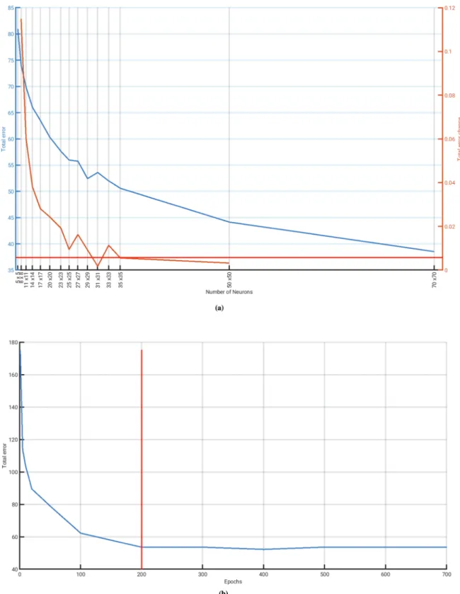
The approximation M=843 corresponds to a 29×29 neuron lattice, which formed the starting point for our optimization. The optimal number of neurons corresponds to the first neuron lattice size where the total error does not decrease significantly when further neurons are added, with the threshold for improvement in the total error being 5% of the initial performance gradient (see supplement in Fendereski et al., 2014). To identify the optimal lattice size, we trained SOMs with different values for M ranging between 25 (5×5) and 4^′900 (70×70) neurons (Fig. A.9), and compared them to one another in terms of their

total error (Fendereski et al., 2014), defined as the sum of the topolog- ical error (TE; Kiviluoto, 1996) and the Manhattan distance based quantization error (QE; Kohonen, 2001; Section A.1). A lattice size of 31×31 neurons (M =961) was identified as the optimal lattice size (Fig. A.9a).

The optimal number of epochs was determined by evaluating the total error of the standard 31×31 lattice as a function of the number of epochs, i.e. where the number of data presentations ranged between [1, 1000](Fig. A.9b). The optimal number of epochs was determined to be 200, since a further increase in the number of epochs did not reduce the total error (Fig. A.9b). As these appear to be the optimal settings for our SOM in relation to the phytoplankton presence projections, for the remainder of the study we only used SOMs with a lattice size of 31×31 neurons, 200 epochs, and the Manhattan distance as its similarity metric. Using this SOM, we performed a first dimensionality reduction of the phytoplankton presence projections, which formed the basis of our subsequent analysis.

2.3. Clustering and identification of the optimal number of clusters A major challenge in cluster analysis is the objective determination of an optimal number of clusters (Xu and II, 2005), which best sum- marizes the dataset in question (Milligan and Cooper, 1985; Vesanto and Alhoniemi, 2000; Salvador and Chan, 2004; Oliver, 2004; Fendereski et al., 2014). We used a K-fold cross validation approach to determine the optimal number of clusters, to avoid both over-generalization and overfitting of data (Sugar and James, 2003; Zaki et al., 2014; Aggarwal, 2015).

The optimal number of clusters was identified through four sets of K- fold cross-validation experiments. K was set to ten, five, three, and two, i.e. the fraction of data left out in the training process was increased from 10% to 20%, 33%, and 50% (Fig. 1; De’ath and Fabricius, 2000;

Zaki et al., 2014; Fendereski et al., 2014; Aggarwal, 2015). The cross- validation experiments consisted of three steps: (i) splitting of the data into K equally sized, randomly chosen, non-overlapping subsets prior to training one SOM on K-1 of these subsets, (ii) clustering of the trained neurons of the SOM into 2 to 100 clusters, and (iii) predicting the data structure of the remaining subset of the data (i.e. of the data left out).

This procedure was repeated until all K subsets were used K-1 times for training, and once for validation.

In step (i), we trained ten, five, three, and two optimized SOMs (Section 2.2) with 90%, 80%,66%, and 50% of the 1^◦×1^◦pixels with phytoplankton species composition projections, respectively. For each SOM, this resulted in 961 trained neurons with a specific biogeographic phytoplankton species composition presence-absence pattern (consisting of 536 species). This step group the phytoplankton species presence data into a 961×536 matrix. This means that each of the 961 neurons is representative for a subset of the global monthly grid cells with phytoplankton community projections.

Following step (i), we performed an additional dimensionality reduction of the 961×536 matrices through a principal component analysis (PCA; Abdi and Williams, 2010). This step was necessary, since the performance of clustering algorithms generally decreases with an increasing number of features (here defined by the total number of projected species; N=536 Bellman, 2015), and the number of neurons (M =961) should significantly exceed the number of projected species that characterize each neuron (Cunningham, 2008). Thus, we projected our 961 trained neurons onto their principal components with an eigenvalue above 1 (Kaiser’s rule; Wilks, 2011).

After reducing the 961×536 matrix through PCA, we applied a hierarchical agglomeration clustering (HAC; Jain et al., 1999) with the Manhattan distance as the similarity metric in step (ii). We used the weighted average-linkage (Hastie et al., 2009), because this linkage is statistically more robust than the complete- or single-linkage clustering (Hastie et al., 2009). Through HAC, we grouped the PCA-transformed neurons into 2 to 100 clusters, which is equal to 99 levels of Table 1

Number of genera and species per phylum/class found in the monthly phytoplankton species presence dataset.

Phylum/Class Number of genera Number of species

Dinoflagellata 61 258

Bacillariophyceae 72 232

Haptophyta 21 32

Chlorophyta 3 4

Cyanobacteria 3 4

Cryptophyta 2 2

Dictyochophyceae 2 2

Chrysophyceae 1 1

Euglenozoa 1 1

(6)

granularity in the clustering. This chosen range in the amount of clusters (2 to 100), includes the amount of biomes and provinces reported previously (e.g. 57 in Longhurst, 2007), while allowing for unanticipated higher—or lower—levels of structural detail than reported in Long- hurst’s scheme or other biome ocean partitionings (e.g. Oliver and Irwin, 2008; Fay and McKinley, 2014; Kavanaugh et al., 2014; Reygondeau et al., 2011; Costello et al., 2017). For each level of granularity, each of the 961 neurons was dynamically associated with one of the available clusters, e.g. for the first level (two clusters) each neuron was either dynamically associated with the first or the second cluster, and the second level (three clusters) each neuron was dynamically associated with one of the three clusters, and so forth.

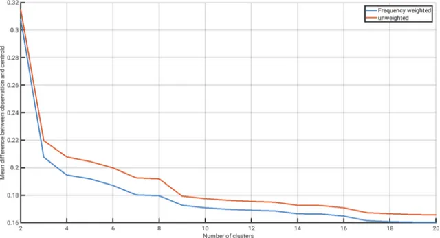
Following Fendereski et al. (2014), we calculated the cluster centroids, to evaluate the goodness of fit of each individual level of granularity tested during the clustering procedure. For each individual cluster at each level of granularity, we calculated the mean of the trained neurons associated with the cluster (without PCA transformation). This mean value was weighted by the number of times a cluster occurred throughout the year (cluster centroids). To this end, we associated each 1^◦-pixel in the validation set to a neuron based on the minimum Man- hattan distance between the community presence of a pixel and the trained neurons. Using the association between neurons and clusters, we then assigned a cluster centroid to each 1^◦-pixel.

During the final step (iii), we calculated the goodness of fit for each level of granularity based on the difference between each 1^◦-pixel in the validation set and its corresponding cluster centroid. This difference was calculated as the mean validation error Dxy for each of the K cross- validation experiments x= [1,K] (K= 10, 5, 3,2), at each level of granularity y= [2,100] (Fendereski et al., 2014). Dxy represents the difference between phytoplankton species presence projections vijxy

contained in the validation dataset and the corresponding predicted cluster centroids wijxy:

Dxy= 1 536

∑⁵³⁶

j=1

( 1 N

∑^N

i=1

|vijxy− wijxy| )

, (2)

where i denotes a specific 1^◦×1^◦pixel in a specific month, j denotes one of the 536 phytoplankton species, and N stands for the number of observations in the validation set (34^′165).

After calculating Dxy for each of our four validation experiments, we calculated an average validation error (Dy) at any given K as follows:

Dy=1 K

∑^K

x=1

Dxy. (3)

We analyzed the evolution of Dy as a function of the increasing number of clusters, and for each fraction of data left out during training (Fig. 1). We identified the minimum number of clusters beyond which Dy

did not decrease by more than 1% relative to the maximum Dy for at least three consecutive increases in the number of clusters (Oliver, 2004). The stagnation in the decline of the mean validation error was reached at ten clusters in the 10-fold cross-validation (Fig. 1a), at eight clusters in the 5-fold cross-validation (Fig. 1b), and at nine clusters in the 3-, and 2-fold cross-validations (Fig. 1c, d). We chose nine clusters as our decisive number of clusters beyond which the mean validation error stagnated, as this value was the mean value of our four cross-validation experiments, and also the result of the most stringent cross-validation tests (i.e. at the largest fractions of data left out; 33%, and 50%).

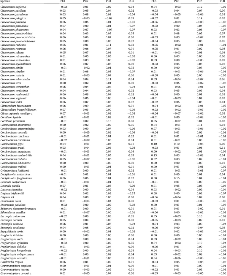
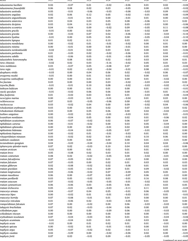
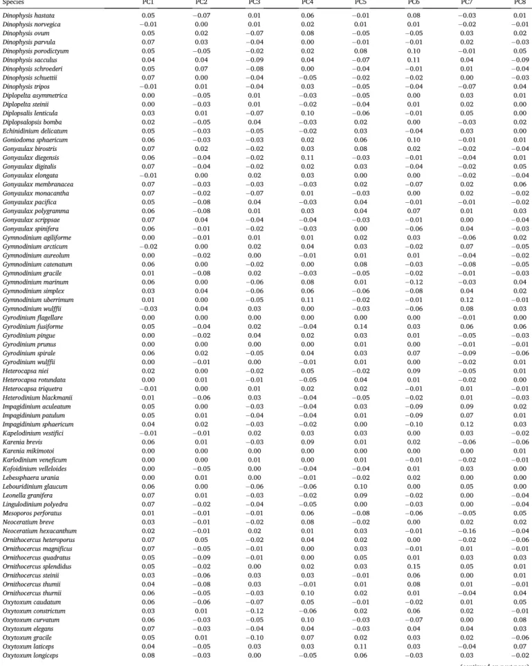
These insights from the cross-validation experiments were used to calculate the final clusters used in all further analyses as follows: first, we trained a new SOM using the entire dataset, which resulted in a 961×536 matrix. Second, we reduced the dimensionality of the 961× 536 matrix to a 961×8 matrix using the principal components found based on Kaiser’s rule (n=8; associated eigenvalue >1; Table A.6). The resulting principal components explained 75.19% of the variance in the trained neurons across all 536 species, where the first three principal components (PCs) captured the majority of the variance (40.89%

explained by PC1; 12.36% by PC2; 7.87% by PC3, 4.69% by PC4, and the remaining 9.38% by PC5 to PC8). Third, we clustered the 961×8 matrix into the optimal number of nine clusters using HAC, and we calculated the cluster centroids for these nine clusters.

2.4. Transforming clusters into biomes and smoothing procedure We assessed the spatial distribution of the nine clusters (Section 2.3) at the monthly, seasonal mean, and annual mean scale. At the monthly scale, we defined spatially coherent biomes that covered at least 0.5% of the surface ocean area. Based on these monthly biomes, we derived biomes at the seasonal and annual scale using the biome that was most frequently predicted at monthly scale, at any particular location, as the seasonal or annual biome, respectively.

To obtain monthly biomes, we eliminated small heterogeneities in the distribution of our nine monthly clusters. Heterogeneities were defined as small patches of a particular cluster that were fully or partly contained within one of the other eight clusters, and with an area below 0.5% of the global surface ocean area. We reassigned these small patches to the cluster with the most similar cluster centroid (as visualized in the dendrogram of Fig. 4a). In cases where reassignment was not possible because patches were surrounded by land or missing Fig. 1.Results of the four K-fold cross- validation experiments with increasing increasing leave-out data, i.e. fractions of the data that are left out during training and spared for validation. The leave-out data amounted to: (a) 10%, (b) 20%, (c) 33%, and (d) 50%. Blue lines show the mean validation error as a function of the number of clusters. Red lines show the mean abso- lute change of the validation error (i.e. the loss in validation error by adding one more cluster). The mean validation error is calculated as the average difference between observations in the validation dataset and the centroid of their corresponding clusters emerging from the training dataset.

(7)

values (e.g. in the Sea of Japan), we assigned a missing value. This reassignment was repeated until each patch was assimilated by another cluster, and the combination covered an area above 0.5% of the available surface ocean area.

To visualize seasonal or annual biomes (integrating three months, or twelve months, respectively), an aggregation of the monthly biomes was needed. To each 1^◦-pixel, we assigned a seasonal biome by selecting the monthly biome that occurred more often than 50% of the months in that season, or over the full year, respectively. If monthly biomes occurred at even frequency in a pixel and season or year, we assigned the phytoplankton community of that pixel to the biome with the most similar cluster centroid. The similarity was defined as the distance between the phytoplankton community matrix and the biome centroids. Potential emerging patches (with area coverage below 0.5% of the global ocean area) were reassigned to the next most similar cluster as described above (smoothing procedure). The aggregation and post-processing of monthly biomes resulted in eight seasonal biomes, and seven annual biomes. We note that one out of the nine monthly biomes only occurred in four months. This biome was not frequent enough to be reflected in seasonal or annual biomes and had overall the least mean spatial coverage (1.2%;

A.8). We thus excluded it from further analysis, leading to a final distinction of eight monthly biomes.

2.5. Robustness assessment of the optimal number of clusters

Next, we assessed the robustness of our classification in terms of its sensitivity to information loss, i.e. we tested whether the optimal number of clusters and their spatio-temporal distribution depended strongly on subsets of the initial training data. To this end, we tested the robustness of our eight biomes to (i) spatial/temporal information loss and (ii) feature (species) loss during training.

First, we assessed the robustness of our classification to loss of spatio- temporal phytoplankton community information. To this end, we retained all 536 species, but trained five optimized SOMs (Section 2.2) on a decreasing fraction of 99%, 95%, 90%, 80%, and 70% of the original monthly 1^◦×1^◦phytoplankton community projections, chosen at random from the original data set (spatial/temporal data loss experiment). Second, we trained five optimized SOMs (Section 2.2) with all monthly 1^◦×1^◦ phytoplankton community projections, but excluded 1%, 5%, 10%, 20%, and 30% of the 536 species chosen at random (species data loss experiment).

The training of the SOMs in both tests resulted in 961 neurons, which we grouped into nine clusters. We calculated the cluster’s spatial monthly distribution, and transformed them into seasonally corrected monthly biomes (Section 2.4). We quantified the robustness of the method with respect to data loss, using the Kappa index of agreement (Cohen, 1960; Landis and Koch, 1977). The Kappa index ranges between one and zero, where a Kappa index above 0.6 indicates a substantial/

good agreement between maps (Landis and Koch, 1977; Monserud and Leemans, 1992; Fendereski et al., 2014). This index has previously been used to assess the robustness of the biogeographic classification of the Caspian Sea (Fendereski et al., 2014), and for the comparison of global vegetation maps (Monserud and Leemans, 1992). Here we used the surface area of the individual 1^◦-pixels to weight the Kappa index. We calculated the average monthly Kappa index between our monthly biomes and those produced using test data (Table 2).

Overall, the average monthly Kappa index ranged between 0.66± 0.06 and 0.85±0.10 in the spatial/temporal data loss experiment, and between 0.72±0.08 and 0.94±0.03 in the species data loss experiment (Table 2). This indicates a substantial (Landis and Koch, 1977; Monserud and Leemans, 1992) agreement between our biomes and the biomes produced using test data. However, in both robustness experiments, the average monthly Kappa index does not decrease monotonically with increasing fraction of missing data. This suggests that the general patterns remain consistent across experiments, but the exact spatial distribution of our biomes in the robustness experiments depended on the data subsets. Additionally, the Kappa index is generally higher in the species loss experiment compared to the spatial/temporal data loss experiment (except for the 70% data loss level; Table 2). Thus our biomes are more sensitive to spatial/temporal data loss than species loss, which is likely due to the decreasing performance of our clustering algorithms with increasing number of features (species) in a given dataset (Bellman, 2015), as randomly removing 1^◦×1^◦-pixels effectively results in an increase of species compared to the available observations.

2.6. Testing our hypotheses

Our hypotheses were tested using the monthly biomes (Section 2.4).

For each biome, we calculated the median number of species found across the months as a proxy for the projected species composition. We visualized the difference between biomes with regard to their phytoplankton species composition using non-parametric multidimensional scaling (Section 2.6.1; NMDS; Clarke, 1993). Indicator species were identified for each biomes using the monthly surface area occupied by the 536 phytoplankton species (Section 2.6.2). The role of species networks was assessed by identifying phytoplankton species that frequently occurred together in the monthly biomes (Section 2.6.3). Finally, we characterized the environmental conditions of the monthly biomes (Section 2.6.4).

2.6.1. Comparison of phytoplankton species composition between biomes To test whether our biomes harbor unique phytoplankton compositions (Townsend et al., 2008), we quantified and inter-compared four aspects of phytoplankton diversity: (i) biome-specific species richness, (ii) taxon-specific diversity, which takes into account the number of species occurring within each phylum and acts as a proxy for dominance of certain taxa, (iii) species composition, i.e. the presence-absence patterns of all species within each biome, and (iv) differences in dominant species across biomes.

To calculate the biome-specific temporal mean diversity, we (i) integrated monthly species richness at the biome scale, i.e. we counted the total number of phytoplankton species across all 1^◦-pixels within each monthly biome (Table A.9). We then calculated the median and interquartile range of the monthly numbers of phytoplankton species per biome across the twelve months. To examine aspect (ii), we calculated the median number and interquartile range of different species per phyla/class separately, across the twelve months (Tables A.10,A.11,A.12).

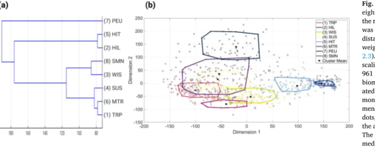
To quantify differences between biomes in terms of species composition (iii), we applied a NMDS (Cardoso et al., 2017; Fendereski et al., 2014) to the species presence-absence patterns contained within each of the trained neurons in our optimal SOM (Section 2.3). The NMDS Table 2

The average and standard deviation of the monthly kappa index of agreement between our biomes and biomes produced using a decreasing fraction of 99%,95%,90%, 80%, and 70% of the original monthly 1^◦×1^◦phytoplankton community projections, chosen at random from the original dataset (Spatial/temporal data loss experiment), and the monthly kappa index of agreement for the comparisons between our biomes and monthly biomes produced after excluding 1%,5%,10%,20%, and 30% of the 536 species chosen at random (Species data loss experiment).

Biome 99% 95% 90% 80% 70%

Spatial/temporal data loss 0.77±0.16 0.78±0.12 0.73±0.17 0.66±0.06 0.85±0.10

Species data loss 0.94±0.03 0.78±0.07 0.76±0.12 0.79±0.11 0.72±0.08

(8)

projects the multidimensional data onto a two dimensional space, where the distances between the projected points correspond to the (dis) similarity in the multidimensional data (Clarke, 1993). We used the Man- hattan distance as our dissimilarity metric of species composition. The NMDS was used to visualize both between-biome differences in species community compositions, and within-biome differences in species community composition. To examine differences between biomes in community composition, we first depicted the core region of each biome in the two-dimensional scaling space. To this end we drew an envelope embracing the 10th to 90th percentile ranges of the species communities of each biome (i.e. we used the median-centered 80% confidence in- terval of species communities, in the two-dimensional scaling space).

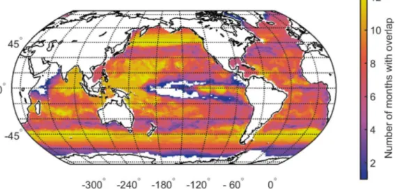
Between-biome differences in the range of community compositions were quantified using the envelope overlap between two biomes (Table A.13). Within-differences in projected species communities were calculated using the spread of the envelope in both dimensions (Table A.14).

To denote dominant species in each biome we determined the distribution and taxonomy of the most frequently found wide-spread species within each biome, i.e. we assumed that species with a large area coverage also represent dominant species. This assumption stems from the observation that the majority of species in our analysis (490 out of 536) are representatives of the comparatively larger-bodied marine micro-plankton (Table 1). The relative representation of species included in our analyses, relative to the total marine phytoplankton species known in the literature, is roughly 7% to 14% (depending on the exact phylum or class). By contrast, smaller-sized plankton groups, containing also less species, are represented by only about 3% of the species known (Righetti et al., 2019a). Thus, our species projections reflect the occurrence patterns of the larger micro-phytoplankton species groups—including functionally important, silicifying Bacillar- iophyceae, calcifying haptophytes, and the large group of dinoflagellates—to a better degree compared to the nano- and pico- pythoplankton.

The original phytoplankton occurrence data remain incomplete with regards to species detection (Cerme˜no et al., 2014), and does not allow us to include particularly rare species into our biome definitions, despite the fact that they account for a large fraction of the local species richness (Ser-Giacomi et al., 2018). Thus, the species for which enough occurrence data were available to train SDMs, are species that have frequently been observed, possibly due higher abundances and commonness.

Frequent species have been shown to account for the majority of phytoplankton biomass or abundance within different phytoplankton groups, with 16 species of coccolithophore out of 195, or 43 diatom species out of 552, accounted for 75% of coccolithophore abundance (O’Brien et al., 2013), or 90% of total diatom biomass (Leblanc et al., 2012), in marine analyses. In addition, common species, unlike rare ones (Ser-Giacomi et al., 2018), have been shown to carry most biogeo- graphical information and ecosystem function (Lyons et al., 2005;

Cermeno et al., 2013), suggesting that their distribution patterns reflect ˜ the ecologically and biogeochemically important processes.

For each biome, wide-spread species were defined as those which rank in the top 100 based on the species’ biome-specific area coverage.

To this end, we calculated the area-weighted fraction of pixels covered by each species within a biome, relative to the total biome area (Table A.19).

2.6.2. Identification of indicator species

In analogy to the flora and fauna characteristic of certain terrestrial biomes (e.g. Picea abies as species typical for the boreal biome; Yang et al., 2020), we explored whether our biomes can be discerned based on indicator species. This analysis served to test the fourth hypothesis, i.e.

that biomes can be characterized through indicator species or species composition (Section 2.6.3).

To assess whether our biomes can be unequivocally identified based on a common, easily identifiable subset of species, we categorized the

phytoplankton species found in each biome using the core-satellite species hypothesis (Hanski, 1982). This hypothesis differentiates between two types of species (Gibson et al., 1999; Ellison, 2019): core species, which are abundant and common (i.e. found in >90% of a region), and satellite species, which are sparse and uncommon (i.e. found in

⩽10% of a region). While the species found between these thresholds are not specified in the core-satellite hypothesis, an extension of this hypothesis recognizes them as subordinate species (Gibson et al., 1999), adopted herein.

To classify a species as a core, subordinate, or satellite species, we calculated the relative presence area for each of the 536 phytoplankton species, based on the 1^◦×1^◦phytoplankton species presence data for each biome in each month (normalized area coverage). The normalized area coverage of each phytoplankton species (ranging between 0 and 1) was used as a proxy for the ubiquity of a species within a biome, i.e. the generality of its spatial presence within a biome. The normalized area coverage of all species per biome was used as a proxy for habitat heterogeneity, where biomes harboring many species with a minor normalized area coverage are more heterogeneous than biomes harboring the same number of species, with each species covering a large relative area. For each biome and month we calculated a vector of 536 species with a number between zero and one specifying the normalized area where the species was present. For each biome, we then calculated the average normalized area from the twelve monthly vectors to visualize the habitat heterogeneity of our biomes.

To identify core, subordinate, and satellite species we used the monthly vectors of the normalized area coverage of the 536 species for each biome and the thresholds mentioned above (Gibson et al., 1999).

Thus, the core, subordinate, and satellite species were identified for each month and each biome, and indicator species were defined as those that are core species in one specific biome (i.e. found in >90% of a biome), and satellite species in all other biomes in a given month (i.e. found in ⩽ 10% of a biome).

2.6.3. Identification of phytoplankton species co-occurrences

We further tested whether the species compositions of our biomes were determined by the potential species co-occurrences derived from the species presence-absence projections, and whether biomes can be identified solely based on a subset of species that characterize biome- specific phytoplankton compositions. For this, we used a text analysis algorithm that identified pairs of species which co-occurred more frequently than expected by chance, given their individual areal coverage (Dunning, 1993; Wahl and Gries, 2018).

The text analysis algorithm assigned an association score to pairs of phytoplankton species found in all 1^◦×1^◦pixels of a biome during all months (Dunning, 1993), reflecting the intensity of links between species. The first step served to construct a contingency table, which contained the number of times both species were present (k11; co- occurrence), the number of times only the second species was present (k12; alternating occurrence), the number of times only the first species was present (k21; alternating occurrence), and the number of times both species were absent (k22; co-absence) at the 1^◦ spatial and monthly resolution per biome. Based on this contingency table, the algorithm used Shannon’s entropy (H), to compare the presence probability of the two species found together against the presence probability of the two species found individually. H is a measure for the uncertainty in the observed probability distribution (Ricotta, 2002; Ricotta, 2005), and is then used to define the following likelihood ratio (LLR; Dunning, 1993):

LLR=2⋅(∑

k)⋅[H(k) − H(kr) − H(kc)], (4)

H(k) =∑kij

klog (∑kij

k )

, (5)

(9)

k=

⎛

⎜⎜

⎝ k11

k12

k21

k22

⎞

⎟⎟

⎠, (6)

kr=

(k11+k12

k21+k22

)

, (7)

kc=

(k11+k21

k12+k22

)

. (8)

The values of LLR are non-negative, and the magnitude of the value indicates the level of significance of the co-occurrence (Dunning, 1993;

Evert, 2009). The differentiation between positive (k11) and negative (k12, k21, k22) associations is done by multiplying the LLR by − 1, if the observed occurrence frequency of the species pair is lower than the product of occurrence frequencies of the individual species divided by the sample size (i.e. the total amount of pixels in a biome across all months; Evert, 2009). Thus, negative values indicate pairs of species that co-occur less than the product of occurrence frequency of the individual species (i.e. the expected co-occurrence).

This procedure resulted in a 536×536 matrix with the LLR-values for all possible species pairs per biome and month. As our goal was to find species co-occurrences characteristic to individual biomes, we were interested in significant species pairs, i.e. species pairs with positive co- occurrences in one biome and alternating occurrences or co-absences in all other biomes. Additionally, the positive co-occurrences should be common for a biome (i.e. the pairs should be present in most of the biome area). For each month, common positive co-occurrences were those with a positive LLR-value and a minimum area coverage (cf.

Section 2.6.2) of the involved species above the 90th percentile of the area coverage of individual species in that biome. Alternatively, uncommon or rare co-occurrences were those with a negative LLR-value or a minimum area coverage of the involved species below the 10th percentile of the area coverage of individual species in all other biomes.

We used the area coverage approach to exclude species pair that had a large LLR value, yet were only present in a few 1^◦-pixels of a biome.

Next, we defined species co-occurrences that consisted of at least two significant species pairs with strong co-occurrences. For instance, a strong co-occurrence of species A and B, and species A and C represented a co-occurrence consisting of A, B, and C.

Finally, we used the presence distribution of all species that formed significant pairs in this analysis to train a SOM and produce biomes. The monthly spatial patterns of these biomes were compared to those of the original biomes based on the area overlap between the biomes of both clusterings. This resulted in a measure of how well the biomes were represented using only the selected species co-occurrences.

2.6.4. Biome-specific differences in environmental conditions

To identify variables that could facilitate biome monitoring through easily measurable environmental (e.g. using satellites or Argo-floats), rather than biological properties, we inter-compared prevailing environmental conditions at the biome scale. Any statistically significant biome differences in measurable environmental parameters such as sea surface temperature, chlorophyll-a concentration, or light could serve to compare our ocean partitioning to previous biogeochemical ocean classifications (e.g. Fay and McKinley, 2014; Gregor et al., 2019; Zhao et al., 2019).

We consider the ten core environmental predictors used to model the species’ presence-absence distribution (Righetti et al., 2019a), and net primary production at monthly climatological 1^◦-resolution (Table A.5):

sea surface temperature (SST; Locarnini et al., 2013), surface nitrate (N;

Garcia et al., 2013), phosphate (P; Garcia et al., 2013), silicic acid (Si;

Garcia et al., 2013) concentration, sea surface salinity (SSS; Zweng et al., 2013), photosynthetic active radiation (PAR; NASA, 2018b), surface chlorophyll-a concentration (chl; NASA, 2018a), mixed layer depth

(MLD; Mont´egut, 2004), net primary production (NPP; Behrenfeld and Falkowski, 1997, 2008, 2017), sea surface wind stress (wind; Atlas et al., 2011), sea surface CO2 partial pressure (pCO2; Landschützer et al., 2014). In addition to the eleven variables listed above, we considered excess phosphate (P*; Deutsch et al., 2007) using the surface nitrate and phosphate concentrations.

To identify a set of environmental variables suitable for the distinction of phytoplankton-based biomes, we tested for differences in individual environmental parameters between our biomes, using a Kruskal- Wallis test (Wilks, 2011). We tested whether biomes differed in their distribution of these environmental parameters at the 1% significance level using all 1^◦-pixels of each biome across all months (Fig. A.18). For those environmental parameters in which at least one biome differed from all others, we compared the environmental conditions between each pair of biomes (p⩽0.01) with a Tukey-Kramer multi-comparison test (Kramer, 1956). For each month, and each pairwise comparison between biomes, we counted the number of months where we could not differentiate between the two biomes based on each environmental factor. Lastly, for each biome we determined a set of two environmental parameters that were best suited to separate this biome from all others.

Thus, for each combination of two environmental factors we counted the number of months where we could not differentiate between two biomes using either one or both environmental factors individually.

3. Results

3.1. Can the open ocean be partitioned into ecologically relevant biomes based on phytoplankton species biogeography?

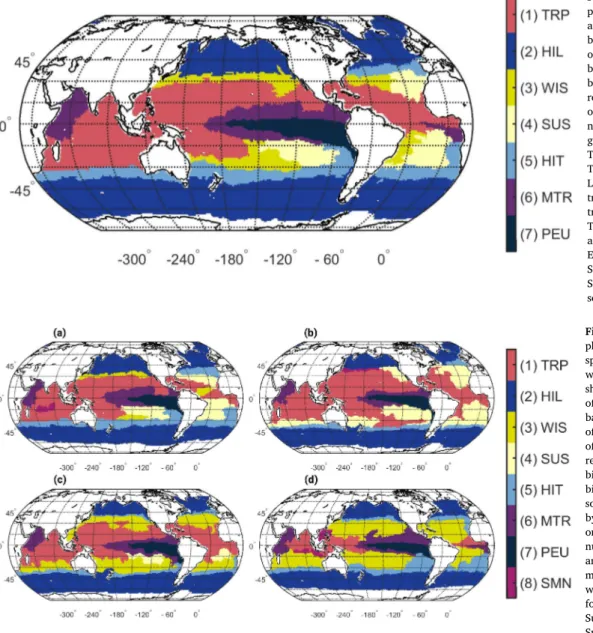
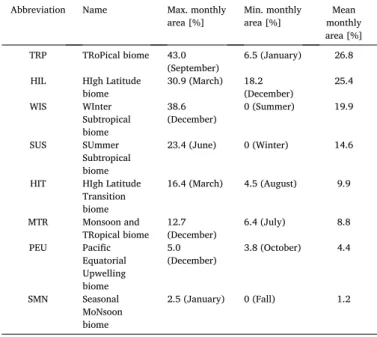
We predict a partitioning of the open ocean into seven statistically separable annual biomes (Fig. 2), which are derived from eight seasonal and monthly biomes. This partitioning shows a clear differentiation between the high latitudes and the low latitudes. Overall, we found three tropical biomes, one high-latitude biome, one transitional biome between the high-latitudes and lower latitudes, two seasonally alternating subtropical biomes and a tropical/temperate biome that is absent on the annual scale, but present during spring, summer, and winter (Fig. 3). The dynamic nature of the seasonal biomes is mostly seen around the subtropics (Fig. A.15), and evident for all seasons, where between 15.8% (spring) and 37.4% (winter) of the 1^◦-pixels have a different biome association relative to the annual distribution.

The TRoPical biome (TRP) is found equatorward of 30^◦ in both hemispheres of the Indian, Pacific, and North Atlantic Ocean (Fig. 2).

TRP covers 26.8% of the surface open ocean in the annual analysis (Table 3). It is largest in summer (39.0%), where it extends between 42^◦N and 40^◦S (Fig. 3b), and smallest in winter (8.3%), where it stretches from 21^◦N to 18^◦S (Fig. 3d).

The HIgh Latitude biome (HIL) extends from the poles to around 40^◦ in both hemispheres (Fig. 2) and covers 25.4% of the surface open ocean on average (Table 3). The area covered by the HIL biome shows little seasonality (26.3% to 30.1%; Fig. 3). Differences between seasons are linked to the loss and gain of 1^◦×1^◦ projections available poleward from 60^◦in the Southern Hemisphere and the North Atlantic Ocean.

The WInter Subtropical biome (WIS) is located in the Pacific and Atlantic Oceans (Fig. 2), and covers on average 19.9% of the surface open ocean (Table 3). This biome is largest in winter (31.1%) and is found between 30^◦ and 5^◦ in both hemispheres in all ocean basin (Fig. 3d). The WIS biome is absent during all summer months (Table A.8).

The SUmmer Subtropical biome (SUS) is located in the Pacific and Atlantic Oceans (Fig. 2), and covers 14.6% of the surface open ocean in the annual analysis (Table 3). Similarly to the WIS biome, it varies in size between seasons. SUS is absent during winter months (Table A.8) and is largest in summer (18.8%), where it is located between 15^◦and 45^◦in the Atlantic Ocean and South Pacific, and between 30^◦and 45^◦in the Indian and North Pacific Ocean (Fig. 3b).

(10)

The HIgh latitude Transition biome (HIT) is located between 30^◦and 40^◦in both hemispheres of all ocean basins, except for the North Pacific Ocean (Fig. 2). It covers on average 9.9% of the surface open ocean (Table 3), with little seasonality. HIT is largest in winter (14.0%; Fig. 3d) and smallest in fall (4.7%; Fig. 3c).

The Monsoon and TRopical biome (MTR) is located in the Arabian Sea and around the Pacific and Atlantic Eastern equatorial region between 15^◦N and 15^◦S (Fig. 2). MTR covers on average 8.8% of the global surface ocean area (Table 3). The location and extent of the MTR biome remains relatively constant throughout the seasons with maximum area coverage in winter (10.5%; Fig. 3d) and minimum area coverage in summer (6.1%; Fig. 3b).

The Pacific Equatorial Upwelling biome (PEU) is located in the Pa- cific Eastern equatorial region (Fig. 2). PEU covers on average 4.4% of the surface ocean area, and its area displays little seasonality (Fig. 3).

PEU is largest in summer (4.4%; Fig. 3b) and smallest in fall (3.8%;

Fig. 3). In spring and fall (Fig. 3a and c), PEU extends to 150^◦W, and in summer and winter (Fig. 3b and d) it extends to 180^◦W.

The Seasonal MoNsoon biome (SMN) does not appear on the annual scale, but it is present during spring, summer and winter in the Indian

and Pacific Oceans (see Fig. 3a,b,c). SMN covers on average 1.2% of the surface ocean area. SMN is largest in winter (1.7%) where it is located in the Central Indian Ocean around 10^◦S, and the South China Sea (Fig. 3d). In spring, it is located in the Central Indian Ocean at 15^◦S as a small patch (1.0%; Fig. 3a). In summer, the SMN biome is located at the boundary between TRP and HIL in the North Pacific Ocean (0.6%;

Fig. 3b).

In summary, phytoplankton-based biomes divide the ocean into tropical and high latitude biomes, with more complexity found in the tropical latitudes. Four biomes are characterized by a rather constant extent throughout the year (HIL, HIT, MTR, and PEU), and four biomes are variable in their spatio-temporal extent (TRP, WIS, SUS, and SMN).

WIS and SUS transcend ocean basins, or vanish for an entire season. SMN is the smallest and temporally most variable biome as its location changes in each season.

3.2. How do biomes differ in terms of their overall and taxon-specific diversity?

In a first step we assessed differences in species richness between Fig. 3.Seasonal distribution of our phytoplankton-based biomes in (a) spring, (b) summer, (c) fall, and (d) winter. The Southern Hemisphere was shifted by six months for the calculation of the seasonally integrated biomes based on the monthly scale distribution of our biomes. The seasonal distribution of each biome was based on the respective monthly distribution of the biome, assigning the most frequent biome to each 1^◦-pixel. The final seasonal biome boundaries were smoothed by reducing the patchiness of initial biomes (Section 2.4). Biomes are numbered according to their mean annual geographic coverage across months. The following abbreviations were used: TRP for TRoPical biome; HIL for HIgh Latitude biome; WIS for WInter Subtropical biome; SUS for SUmmer Subtropical biome; HIT for HIgh latitude Transition biome; MTR for Monsoon and TRopical biome; PEU for Pacific Equa- torial Upwelling biome; SMN for Seasonal MoNsoon.

Fig. 2. Annual distribution of phytoplankton-based biomes. The annual distribution of each biome was based on monthly distributions of biomes, assigning the most frequent biome to each 1^◦-pixel. The final annual biome boundaries were smoothed by reducing the patchiness of initial biomes (Section 2.4). Biomes are numbered according to their mean geographic coverage across months.

The following abbreviations were used:

TRP for TRoPical biome; HIL for HIgh Latitude biome; WIS for WInter Sub- tropical biome; SUS for SUmmer Sub- tropical biome; HIT for HIgh latitude Transition biome; MTR for Monsoon and TRopical biome; PEU for Pacific Equatorial Upwelling biome; SMN for Seasonal MoNsoon biome. Note that the SMN biome is absent on the annual scale.