Article
Evaluation of the Sea-Ice Simulation in the Upgraded Version of the Coupled Regional Atmosphere-Ocean- Sea Ice Model HIRHAM–NAOSIM 2.0
Wolfgang Dorn1,* , Annette Rinke1 , Cornelia Köberle2, Klaus Dethloff1 and Rüdiger Gerdes2,3
1 Alfred Wegener Institute, Helmholtz Centre for Polar and Marine Research, Telegrafenberg A45, 14473 Potsdam, Germany
2 Alfred Wegener Institute, Helmholtz Centre for Polar and Marine Research, Klußmannstraße 3d, 27570 Bremerhaven, Germany
3 Physics and Earth Sciences, Jacobs University , Campus Ring 1, 28759 Bremen, Germany
* Correspondence: Wolfgang.Dorn@awi.de
Received: 5 June 2019; Accepted: 23 July 2019; Published: 26 July 2019
Abstract:The sea-ice climatology and sea-ice trends and variability are evaluated in simulations with the new version of the coupled Arctic atmosphere-ocean-sea ice model HIRHAM–NAOSIM 2.0.
This version utilizes upgraded model components for the coupled subsystems, which include physical and numerical improvements and higher horizontal and vertical resolution, and a revised coupling procedure with the aid of the coupling software YAC (Yet Another Coupler). The model performance is evaluated against observationally based data sets and compared with the previous version. Ensemble simulations for the period 1979–2016 reveal that Arctic sea ice is thicker in all seasons and closer to observations than in the previous version. Wintertime biases in sea-ice extent, upper ocean temperatures, and near-surface air temperatures are reduced, while summertime biases are of similar magnitude as in the previous version. Problematic issues of the current model configuration and potential corrective measures and further developments are discussed.
Keywords:Arctic sea ice; coupled atmosphere-ocean-sea ice model; regional modeling
1. Introduction
Coupled regional atmosphere-ocean-sea ice models provide the possibility of simulating interactions and feedback between their components which often occur at regional fine spatial and temporal scales that are not resolved by global models. Such feedback between atmosphere, sea ice, and ocean plays a critical role in the evolution of the Arctic climate system and is likely to be jointly responsible for the climate phenomenon called Arctic Amplification [1]. The best known feedback in the Arctic climate system is the ice–albedo feedback, but a variety of other feedback exists, much of which is not yet understood in detail such as the feedback between sea ice and cyclones.
A coupled regional climate model can be an especially useful tool for providing information on the mechanisms behind the feedback between the atmosphere, sea ice, and ocean and for testing different parameterizations of processes involved in such feedback. The regionally limited model domain with its constrained lateral boundary conditions is a major advantage in this regard, since the model does not need to show reasonable performance in simulating global teleconnections. For instance, the simulation of the Atlantic Meridional Overturning Circulation (AMOC), which can sometimes be problematic in global circulation models [2,3], is not a major issue for a regional model with prescribed boundary conditions. However, the coupled regional climate model has to rely on the atmospheric and oceanic data used as lateral boundary forcing. This is a particular issue for the lateral ocean boundary
Atmosphere2019,10, 431; doi:10.3390/atmos10080431 www.mdpi.com/journal/atmosphere
and represents a limitation of coupled regional climate models in adequately reproducing observed climate changes.
Here, we first describe the upgraded version of the coupled Arctic atmosphere-ocean-sea ice model HIRHAM–NAOSIM (HN2.0) that succeeds the previous version (HN1.2). HN2.0 utilizes upgraded components, which include physical and numerical improvements and higher horizontal and vertical resolution, and a completely revised coupling procedure. The first version of HIRHAM–NAOSIM (HN1.0) was described by Rinke et al. [4]. Subsequent minor upgrades of the model (henceforth referred to as HN1.1 and HN1.2) were described by Dorn et al. [5] and Dorn et al. [6]. The present major upgrade of the coupled model was performed in the framework of the “ArctiC Amplification:
Climate Relevant Atmospheric and SurfaCe Processes, and Feedback Mechanisms (AC)3” project with the aim to investigate interactions between atmosphere and sea ice in the Arctic [7]. Details of the model components and to the coupling are given in Section2, while a basic evaluation of the current “base” configuration of HN2.0, which focuses mainly on sea ice as the communicator between atmosphere and ocean, is given in Section3. Major improvements as compared to the previous version (HN1.2) as well as known weaknesses and potential further development of the model are discussed and summarized in Section4. It should be noted that the current base configuration is designed to serve as a reference for contemplated improvements of interaction processes between atmosphere, sea ice, and ocean.
2. Description of HN2.0
HIRHAM–NAOSIM 2.0 consists of the regional atmospheric climate model HIRHAM5 and the regional ocean-sea ice model NAOSIM. The atmospheric component HIRHAM5 comprises both a new dynamical core and a new set of physical parameterizations (compared to HIRHAM4 in HN1.x) and is set up with horizontal resolution of 0.25◦and 40 vertical levels (compared to 0.5◦and 19 vertical levels in HN1.x). The ocean-sea ice component NAOSIM includes only a few physical, but several technical improvements, and it is set up with horizontal resolution of 1/12◦and 50 vertical levels (compared to 0.25◦and 30 vertical levels in HN1.x). Since the dynamical cores and the physical parameterizations of the two components were already explicitly described in scientific documentations or respective reference manuals, the focus here will be to explain the adaptations made in HN2.0 with respect to the original formulations of the model components and to detail the coupling between HIRHAM5 and NAOSIM. Modifications of physical parameterizations, motivated to improve the model performance in the Arctic, will be explained as well. Information on the code availability of HN2.0 is given in AppendixD.
2.1. Atmosphere Model HIRHAM5
The regional atmospheric climate model HIRHAM5 succeeds the previous version HIRHAM4 [8] that represented the atmospheric component in HN1.x. HIRHAM5 has already been used in a number of climate studies for the Arctic (e.g., [9–14]) and for other regions of the Earth (e.g., [15–20]).
A technical description of the model is given by Christensen et al. [21].
2.1.1. Model Components
HIRHAM5 consists of the hydrostatic dynamical core from the time integration module of the weather forecast system HIRLAM-7.0 [22] and the physical parameterizations of the atmospheric general circulation model ECHAM-5.4.00 [23]. The communication between the HIRLAM and ECHAM5 routines is handled by a separate interface, whereby most of the original model code could be adopted as it stands.
Compared to the original HIRLAM-7.0 code, HIRHAM5 includes technical modifications related to the data management, especially with respect to input and output data and restart functionality as detailed by Christensen et al. [21], and to the separation of cloud water into liquid water and ice.
The latter is required by the ECHAM5 physical parameterizations and was realized by writing cloud
liquid water on HIRLAM’s total cloud water variable and cloud ice on HIRLAM’s first optional tracer variable. The code was consequently modified such that the first tracer variable is treated in exactly the same way as the original total cloud water variable. The bottom line is that HIRHAM5 solves prognostic equations for seven instead of six variables, namely surface pressure, two horizontal wind components, temperature, specific humidity, cloud water, and cloud ice.
Compared to the original ECHAM5 code, technical modifications in HIRHAM5 were kept to a minimum, but could not fully be avoided. Due to different grid definitions in the regional model (rotated spherical grid) as compared to the global ECHAM5 model (Gaussian grid), adaptations were necessary with respect to the initialization of radiation, ozone, aerosols, and soil parameters.
Furthermore, a new data module was introduced in order to store additional output variables from the ECHAM5 physics beyond the usual HIRLAM output.
2.1.2. Modified Parameterizations
The physical parameterization package of ECHAM5 consists of parameterizations for radiation, stratiform clouds, cumulus convection, subgrid scale orography and gravity waves, surface fluxes and vertical diffusion, and surface processes [23]. Compared to the ECHAM4 parameterizations [24]
used in HN1.x, the ECHAM5 parameterizations include a new longwave radiation scheme, separate prognostic equations for cloud liquid water and cloud ice, a new cloud microphysical scheme and a prognostic-statistical cloud cover parameterization as specified by Roeckner et al. [23]. In addition, the number of spectral intervals is increased in both the longwave and shortwave part of the spectrum, and changes have been made in the representation of land surface processes, including an implicit coupling between the surface and the atmosphere, and in the representation of orographic drag forces (see [23] for details). Furthermore, the surface fluxes are calculated separately for land, open ocean, and ice-covered ocean as a standard feature. The latter represents a clear advantage for the coupling with an ocean-sea ice model that needs atmospheric fluxes for different surface types.
Within the framework of the development of HN2.0, a few ECHAM5 parameterizations were modified to improve the model performance in the Arctic. These modifications are based on earlier work with HN1.2 or HIRHAM5, respectively, as detailed in the following paragraphs.
The most important modification concerns the surface albedo parameterization and was carried over from HN1.2. The original snow albedo for non-forested land areas was replaced by the polynomial temperature dependency derived by Roesch [25]. For the sea-ice albedo, suggestions by Køltzow [26], which particularly include the effect of melt ponds, were implemented. Version 1 of the sea-ice albedo scheme of Køltzow [26] was implemented for HIRHAM5 stand-alone simulations, while version 2 was implemented for coupled HIRHAM–NAOSIM simulations. The main difference between version 1 and version 2 is the additional consideration of a snow cover fraction in version 2 which is derived in the coupled mode from NAOSIM’s prognostically computed snow thickness. A detailed description of the sea-ice albedo scheme in HIRHAM–NAOSIM was already given by Dorn et al. [6]. HN2.0 includes two modification: First, the linear transition towards the water albedo for thin ice (see [6], Equation (33)) is not yet activated; second, the restriction of the melt pond fraction to the sea-ice surface not covered with snow (see [6], Equation (37)) was attenuated such that, at least 25% of the computed melt pond fraction is allowed. The second modification was done to overcome low sea-ice melt rates in early summer when the incoming shortwave radiation is at the maximum and a high amount of snow is still present. The value of 25% can be considered as a tuning value. A more realistic parameterization of the fractions of snow and melt ponds should be derived from observations. This will be subject of future development (see also Section4).
The second modification concerns the stratiform cloud parameterization and includes a more efficient Bergeron–Findeisen process and a more generalized subgrid-scale variability of total water content. The main aim was to improve the simulation of low stratiform mixed-phase clouds, since these clouds occur frequently during all seasons in the Arctic [27]. A detailed description of the modified cloud parameterization is given by Klaus et al. [10] who showed that this modification leads to
significant improvements in the simulation of Arctic clouds and the surface radiation budget in HIRHAM5. This modification was implemented as an option and can be switched on or off (currently switched on in HN2.0).
The third and last modification concerns the calculation of the sea-ice temperature and only takes effect in a coupled mode with NAOSIM. In that case, the sea-ice temperature is calculated from the surface energy balance according to the description of the ice growth parameterization by Dorn et al. [6]. The key change to the original ECHAM5 parameterization relates to the heat capacity of the uppermost snow/ice layer (see [6], Equations (21)–(23)). The computation of the heat capacity is substantially the same as in HN1.2, butδh0= 0.05 m is set as the maximum thickness of the uppermost snow/ice layer, motivated by the longer time step in HN2.0 as detailed below.
2.1.3. Domain and Discretization
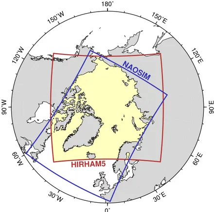
The model domain of HIRHAM5 covers the whole Arctic north of about 60◦N (see Figure1) and is defined in a rotated spherical coordinate system with the North Pole on the geographical equator at 180◦E. The longitude range in the rotated pole grid is from 27.375◦W to 26.875◦E, and the latitude range is from 25.125◦S to 24.625◦N. The horizontal resolution is 0.25◦(approximately 27 km), resulting in a horizontal grid with 218×200 grid points. The dynamical core uses an Arakawa C-grid for the horizontal discretization. This means that the horizontal wind components are staggered in the horizontal with respect to the other prognostic variables that are discretized on the grid given above. In concrete terms, the longitudinal (latitudinal) wind component is staggered by half a grid point distance in longitudinal (latitudinal) direction. HIRLAM internally handles the staggering and de-staggering of the horizontal wind components so that finally all variables are defined at the same grid points.
180˚
150˚W
120˚W
90˚W
60˚W
30˚W
0˚
30˚E
60˚E
90˚E
120˚E 150˚E
HIRHAM5
NAOSIM
Figure 1. Geographical location of the regional model domains of the atmosphere component HIRHAM5 and of the ocean–ice component NAOSIM. The coupling domain is indicated by the yellow area and comprises 20,583 (out of 43,600) HIRHAM5 grid cells and 200,951 (out of 366,850) NAOSIM grid cells.
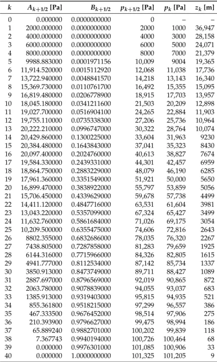
The vertical discretization is given in hybrid terrain-following/pressure coordinates with 40 levels from about 10 m above the surface up to a pressure level of 10 hPa (see AppendixA). The highest vertical resolution is in the lower troposphere, where the lowermost 1 km is represented by 10 levels (see TableA1). A 60-level version, with 20 additional levels in the stratosphere, is also available, but currently not used in coupled mode.
In addition to the traditional Eulerian time stepping scheme (as used in the previous versions), HIRLAM-7.0 includes a semi-implicit semi-Lagrangian scheme. The semi-Lagrangian scheme allows for longer time steps and is now the default. Simulations presented in this paper were carried out with a time step of 600 s. Note that with the Eulerian scheme a time step of about 120 s would have been needed.
2.1.4. Boundary Forcing
At the lateral boundaries, HIRHAM5 is currently driven by data from the ERA-Interim (ERAI) reanalysis [28]. The ERAI data at 6-hourly resolution were downloaded from the Meteorological Archival and Retrieval System (MARS) at the European Centre for Medium-Range Weather Forecasts (ECMWF) and horizontally and vertically interpolated to the regional model grid. The lateral boundary forcing includes all seven prognostic variables. All prognostic variables are treated equally using a 10-grid-point lateral boundary relaxation following Davies [29]. An inflow/outflow formulation for specific humidity, cloud water, and cloud ice is optionally available, but leads occasionally to numerical instabilities due to sharp differences between the imposed boundary values and the modeled values at the adjacent grid points.
At the lower boundary, HIRHAM5 uses sea surface temperature and sea-ice concentration from daily ERAI fields for the sea grid points outside the coupling domain. Note that only a few HIRHAM5 sea grid points close to Pacific coasts are not covered by NAOSIM. Inside the coupling domain, sea surface temperature, sea-ice concentration, sea-ice thickness, snow thickness on ice, and the freezing temperature of sea water are transferred from NAOSIM to HIRHAM5 at 1-h intervals. Outside the coupling domain, fixed values are used for the sea-ice thickness (2 m), the snow thickness on ice (0 m), and the freezing temperature of sea water (271.38 K).
2.2. Ocean-Sea Ice Model NAOSIM
The ocean–ice component of HN2.0 is the fine-resolution model (FRM), introduced by Fieg et al. [30], from the North Atlantic/Arctic Ocean Sea-Ice Model (NAOSIM) hierarchy, whereas the earlier versions (HN1.x) have used the high-resolution model (HRM) of NAOSIM. A basic description of NAOSIM is given by Köberle and Gerdes [31]. Differences between FRM and HRM are described by Fieg et al. [30]. Beyond differences in the model resolution, as stated above, HN2.0 explicitly includes the inflow of freshwater from Arctic rivers and marginal seas, as specified below, while HN1.x simply applies salinity restoring with a time constant of 180 days [5]. The FRM version of NAOSIM has already been used in a couple of Arctic climate studies (e.g., [32–34]). Information on recent technical modifications is given in AppendixB.
2.2.1. Ocean Component
NAOSIM’s ocean component is based on the Geophysical Fluid Dynamics Laboratory Modular Ocean Model MOM-2 [35] and includes prognostic equations for horizontal velocity components, potential temperature, and salinity. The equations of motion are formulated in compliance with the Boussinesq, hydrostatic, and rigid lid approximations. The horizontal velocity components are divided into a depth dependent internal mode velocity, representing the baroclinic flow, and a depth independent or external mode velocity, representing the barotropic flow. The rigid lid approximation at the ocean surface implies that the barotropic mode is non-divergent which allows the external mode velocity to be expressed in terms of a stream function. This barotropic stream function is obtained
by iteratively solving the external mode elliptic equation using a conjugate gradient solver (see [35]
for details).
The advection of tracers (potential temperature and salinity) is calculated using a flux-corrected transport scheme [36,37], which is characterized by low implicit diffusion. Explicit diffusion of tracers is optionally available, but is currently not applied in HN2.0, neither in horizontal nor in vertical direction. Horizontal friction is implemented as a biharmonic diffusion of momentum with a diffusion coefficient of−0.5·1011m4s−1(compared to−0.5·1013m4s−1in HN1.2). Vertical friction is taken to be constant with a kinematic viscosity coefficient of 0.001 m2s−1(as in HN1.2). The bottom drag coefficient is set to 1.2·10−2(compared to 1.2·10−3in HN1.2).
2.2.2. Sea-Ice Component
The sea-ice component is based on the dynamic–thermodynamic sea ice model described by Harder et al. [38] and represents an upgrade of the original Hibler [39] model. Ice concentration, mean ice thickness (ice volume per area), mean snow thickness (snow volume per area), and ice age are computed from extended continuity equations and the ice drift velocities from the momentum balance where the inertia term is neglected. The internal stress is described by a viscous-plastic rheology according to Hibler [39], whereas HN1.2 has used the elastic-viscous-plastic (EVP) rheology described by Hunke and Dukowicz [40] that represents a numerically efficient variant of the viscous-plastic rheology by including some artificial elasticity to enable an explicit stress calculation (see [41] for a review). Since the implementation of a different sea-ice rheology is challenging from a computational point of view, the EVP scheme has not yet been included in HN2.0.
Thermodynamic processes are handled using the zero-layer approach by Semtner [42]. This means that there is no explicit snow or ice layer and neither snow nor ice temperatures are calculated. HN2.0 includes two thermodynamic ice growth schemes: The original scheme, where thermodynamic changes of ice and snow are derived from the energy balance of the combined ocean mixed layer–sea ice system (see [5]), and an upgraded version of the flux-separating scheme of HN1.2 developed by Dorn et al. [6].
The main purpose of upgrading the flux-separating scheme was to allow for sublimation of snow and ice in the respective mass balances. This was neglected in HN1.2 due to the unavailability of corresponding coupling variables (see Section2.3). A few minor numerical improvements were also implemented. The original scheme is currently the default for NAOSIM stand-alone simulations, while the flux-separating scheme is the default for coupled HIRHAM–NAOSIM simulations.
2.2.3. Ocean-Sea Ice Coupling
The momentum coupling according to Hibler and Bryan [43] involves a vertical integration of the momentum balance across both media, the sea ice and the uppermost ocean layer. Interfacial stresses do not appear explicitly and the prognostic variable is the mass-weighted mean velocity of both layers.
Internal forces in the sea-ice component enter the overall momentum balance as a stress, much like the wind stress, the common driver of the melange. It is necessary to calculate one velocity separately to include new parameterizations of ocean–ice drag. Castellani et al. [44] introduced a scheme that takes bottom and surface roughness of deformed ice into account (coded but not activated in HN2.0). In the current model configuration, sea-ice roughness is calculated with the Steiner et al. [45] algorithm.
The benefit of the Hibler and Bryan [43] approach is the representation of the total mass divergence near the surface and thus of the vertical Ekman velocities that are essential drivers of the large-scale ocean flow distant from lateral boundaries. On the other hand, the correct advection of oceanic constituents, including nutrients and other tracers, requires the separate knowlege of the ocean velocity. Especially in shallow waters, where the ice thickness becomes comparable to the water depth, uncertainties may arise.
2.2.4. Domain and Discretization
NAOSIM’s model domain encloses the entire Arctic Ocean, the Nordic seas, and the northern North Atlantic with the southern model boundary at approximately 50◦N (see Figure1). The model uses a rotated spherical coordinate system with the North Pole on the geographical equator at 60◦E.
The horizontal resolution is 1/12◦(approximately 9 km). The equations are horizontally discretized on an Arakawa B-grid, meaning that the two horizontal velocity components are staggered compared to the tracer variables (i.e., temperature, salinity) by half a grid point distance in both longitude and latitude directions. For the tracers (velocities), the longitude range in the rotated pole grid is from 20.5417◦W (20.5◦W) to 39.7917◦E (39.8333◦E), and the latitude range is from 20.5417◦S (20.5◦S) to 21.5417◦N (21.5833◦N), resulting in two horizontal grids with 725×506 grid points each. The grids are referred to as the T-grid (for the tracers) and the U-grid (for the velocities).
In the vertical, the model has 50 unevenly spacedz-coordinate levels. The depth of the levels and the corresponding vertical resolution is given in TableA2. Unlike in the horizontal, tracers and velocities are not staggered vertically and consequently discretized at the same depth. The bottom topography was derived from the ETOPO5 data set [46]. ETOPO5 data were interpolated to the rotated model grid using a Gaussian weighting function of the distance to the central point.
The time stepping scheme of NAOSIM is a mixing scheme that mainly consists of a leapfrog time step. At regular intervals, the leapfrog scheme is replaced by an Euler backward time step which is comprised of two half steps, a first forward step and a second step with data from the first step (also known as forward-backward method). Since the execution of two half steps is numerically more expensive, the interval of replacing the leapfrog by an Euler backward time step should be chosen as large as possible. Pacanowski [35] indicates that the default number of 17 time steps between mixing time steps (i.e., every 17th time step is an Euler backward time step, while the others are normal leapfrog time steps) has been empirically established. This number mostly works well in NAOSIM, but the model tends to crash occasionally when solving the external mode elliptic equation for the barotropic stream function. It was found that the choice of a smaller number is a suitable option to avoid a model crash. Owing to these occasionally occurring model crashes, the HN2.0 simulations were running with a different number of mixing time steps, basically meaning that the simulation of the year in which the model crash occurred was repeated with a smaller number of mixing time steps.
However, the time step of the simulations was always the same with 360 s.
2.2.5. Boundary Forcing
At the southern model boundary in the northern North Atlantic, NAOSIM applies an open-boundary condition following the formulation of Stevens [47]. At inflow points, temperature and salinity are currently restored to the Levitus climatology [48,49] with a time constant of 30 days.
The Levitus climatology was chosen to remain comparable to previous NAOSIM stand-alone and HN1.2 simulations. At outflow points, advection of tracers and sea ice is allowed as well as radiation of waves [30]. Other boundaries with substantial inflow of freshwater (Arctic rivers, Baltic Sea, Hudson Bay, Bering Strait, and White Sea) are treated as virtual sinks of salt in the upper 30 m of the ocean (represented by the uppermost three levels).
At the upper boundary, NAOSIM uses daily means of 2-m air and dew-point temperature, cloud cover, precipitation, wind speed, and wind stress components from ERAI for the grid points outside the coupling domain. The ERAI wind stress components were rotated and interpolated to the regional U-grid, while all other ERAI variables were interpolated to the regional T-grid. Prior to the interpolation, ERAI data that represent land areas had been replaced by distance-weighted averages of data from the sea grid points. This was done to avoid the inclusion of data from land areas into the interpolation because surface values over land may differ widely from those over sea, particularly in the case of existing coastal mountains.
Outside the coupling domain, NAOSIM internally calculates the atmospheric surface fluxes from the prescribed atmospheric boundary values using standard bulk formulas (as in
stand-alone mode), based on the formulations for turbulent fluxes and shortwave radiation by Parkinson and Washington [50] and for longwave radiation by Rosati and Miyakoda [51].
In addition, seven ice thickness classes, assuming a linear distribution between zero and twice the mean ice thickness, are used for calculating the atmospheric surface heat fluxes. Note that the coupling domain does not cover a large part of the northern North Atlantic whereby the ERAI forcing is also relevant in coupled mode. Inside the coupling domain, the atmospheric surface fluxes are calculated by HIRHAM5 and transferred at 1-h intervals (see also Section2.3). In HIRHAM5, all fluxes are calculated separately for the open water part and the ice-covered part of the grid cells, but without using ice thickness classes in the heat flux calculation, since this feature is not yet available in HIRHAM5 (see also Section4).
2.3. Coupling Procedure
The earlier versions (HN1.x) did not make use of an external coupler, meaning that the exchange of data between the model components was handled by the respective master processes of the two components through direct communication. Since the complete grid transformation of the data was done by one single process, namely the ocean model’s master process, the coupling in HN1.x represented a bottle-neck for the model’s application on parallel computer systems. Furthermore, there was a misalignment in the timing of the coupling that especially affected the ocean surface fields at the boundary of the coupling domain. Therefore, the coupling procedure has been completely revised for HN2.0.
The coupling of HIRHAM5 and NAOSIM is handled by means of the relatively new and flexible coupling software YAC 1.2.0 (Yet Another Coupler) [52]. YAC allows for parallelized interpolation and communication of coupling fields. The current interpolation stack for all coupling fields consists of a first-order conservative remapping [53] with a fractional area normalization for the interpolation of partially covered source cells, followed by a distance-weighted two nearest neighbor interpolation.
The downstream nearest neighbor interpolation enables allocating of values to all remaining non-land grid cells in case of non-overlapping cells due to the different resolutions and land-sea masks of HIRHAM5 and NAOSIM.
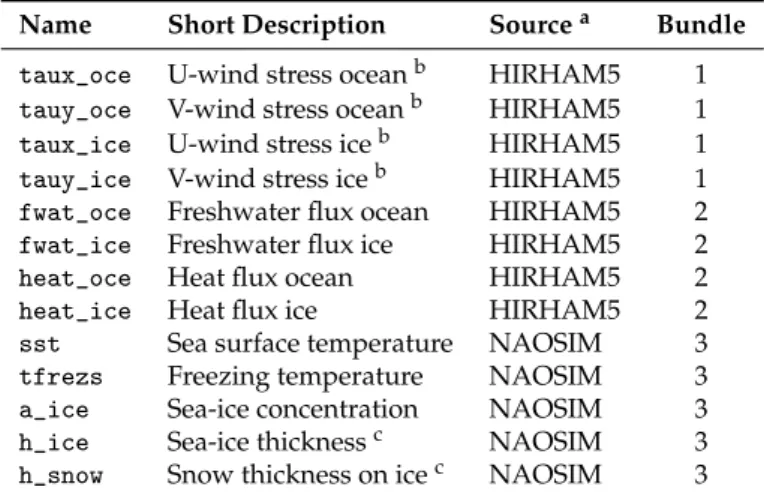
The time step of coupling (currently 1 h for all fields) as well as optional time averaging of coupling fields is managed by YAC. In the current configuration, all fields that are transferred from HIRHAM5 to NAOSIM are averaged over the coupling interval using YAC’s time averaging option, while YAC transfers instantaneous fields from NAOSIM to HIRHAM5. The coupling fields are listed in Table1. The fields that apply to the same source and target grids are transferred in bundles using the same interpolation weights. In HN2.0, the coupling fields are collected in 3 bundles: Bundle no. 1 comprises the fields to be transferred from the HIRHAM5-grid to NAOSIM’s U-grid, bundle no. 2 comprises the fields to be transferred from the HIRHAM5-grid to NAOSIM’s T-grid, and bundle no. 3 comprises the fields to be transferred from NAOSIM’s T-grid to the HIRHAM5-grid.
Wind stress and heat fluxes are provided by HIRHAM5 as potential fluxes (unweighted), while freshwater fluxes are provided as effective fluxes (weighted with the water/ice fraction).
The latter is done in order to reduce the number of coupling fields by two. The freshwater flux over ocean thus includes large-scale plus convective rainfall (assuming that rainfall over ice is directly run off into the ocean) and the open water fraction of evaporation and large-scale plus convective snowfall. Snow falling in open water is directly melted. The required heat of fusion is subtracted from the heat flux over ocean. The freshwater flux over ice is consequently the ice fraction of sublimation and large-scale plus convective snowfall.
The coupling routines have been integrated in HIRHAM5 and NAOSIM via separate modules that provide an interface between the respective model component and YAC (see Figure2). These modules comprise all initialization and working routines required for the exchange of data between the two model components using YAC. To avoid pole problems inherent with the use of conventional geographic coordinates, NAOSIM’s rotated pole grid is treated for the coupling as being a regular
(but limited) latitude-longitude grid and HIRHAM’s longitudes and latitudes are translated into these grid coordinates. The fact that the two rotated grids have their intersection point with the cartesian z-axis at coordinates(0, 0), the geographic North Pole, the coordinate transformation as well as the wind stress rotation can be achieved by a single rotation around thisz-axis (corresponds to the cartesian x-axis when treating the NAOSIM grid as regular grid). In this way, the grid transformation of the coupling fields remains numerically as efficient as possible.
Table 1.List of the coupling fields between HIRHAM5 and NAOSIM.
Name Short Description Sourcea Bundle taux_oce U-wind stress oceanb HIRHAM5 1 tauy_oce V-wind stress oceanb HIRHAM5 1 taux_ice U-wind stress iceb HIRHAM5 1 tauy_ice V-wind stress iceb HIRHAM5 1 fwat_oce Freshwater flux ocean HIRHAM5 2 fwat_ice Freshwater flux ice HIRHAM5 2 heat_oce Heat flux ocean HIRHAM5 2 heat_ice Heat flux ice HIRHAM5 2
sst Sea surface temperature NAOSIM 3
tfrezs Freezing temperature NAOSIM 3 a_ice Sea-ice concentration NAOSIM 3 h_ice Sea-ice thicknessc NAOSIM 3 h_snow Snow thickness on icec NAOSIM 3
aSource indicates the model component in which the field is calculated; the recipient is always the other model component.bWind stress vectors are rotated to the target grid prior to the transfer.cSea-ice thickness and snow thickness are transferred as actual thicknesses unlike the prognostic mean thicknesses (volume per area).
HIRHAM5coupledmode NAOSIMcoupledmode
HIRHAM5
stand-alone atmosphere model
coupling software
YAC
NAOSIM
stand-alone ocean-ice model
mo_couple_naosim
mo_couple_hirham
Figure 2.Schematic diagram of the coupling of HIRHAM5 and NAOSIM using the coupling software YAC (Yet Another Coupler). The boxes “mo_couple_naosim” and “mo_couple_hirham” represent the interface modules between the two model components and YAC.
The coupling domain is basically defined as the overlap area of the components’ model domains (see Figure1). Grid cells that represent land are excluded and masked as uncoupled cells.
The coupling domain in NAOSIM is limited by the outer vertices of the outermost HIRHAM5 grid cells. In HIRHAM5 coordinates, these vertices are at longitudes 27.50◦W and 27.00◦E and at latitudes 25.25◦S and 24.75◦N. NAOSIM grid cells whose HIRHAM5-transformed longitude and latitude fall outside this area are masked as uncoupled cells.
For the coupling domain in HIRHAM5, the outermost NAOSIM grid cells are neglected, since these cells mostly represent a passive boundary. Since HIRHAM5 only receives fields from NAOSIM’s T-grid, the coupling domain in HIRHAM5 is thus limited by the outer vertices of the second outermost NAOSIM T-grid cells. In NAOSIM coordinates, these vertices are at longitudes 20.50◦W and 39.75◦E and at latitudes 20.50◦S and 21.50◦N. Like in NAOSIM, HIRHAM5 grid cells whose NAOSIM-transformed longitude and latitude fall outside this area are masked as uncoupled cells. In both model components, masked grid cells are treated as in stand-alone mode.
3. Evaluation of the Base Configuration
HIRHAM5 as well as NAOSIM can be configured via a number of namelist parameters. For the first coupled simulations with HN2.0, these namelist parameters were carried over from the stand-alone model versions except for the modifications explicitly specified in Section2. Another exception is that the coupled mode flag is activated in the ECHAM5 part of the model. This has the side effect that different default parameters are used in the ECHAM5 physics. In particular, the mixing ratios of greenhouse gases are preset in coupled mode with values for the year 1860. This was actually not intended and basically means that the local greenhouse effect is underestimated in the current HN2.0 simulations which should actually represent the present-day climate. The impact of time-adjusted greenhouse gases will be evaluated at a later date in a new configuration. The current setup of HN2.0 is here taken as a basis and simply referred to as the base configuration (see also AppendixC). Relevant physical constants used in the base configuration are given in TableA3.
3.1. Ensemble Simulation Setup
An ensemble of 10 hindcast simulations were carried out with HN2.0 for the period 1979–2016.
The simulations were driven by ERAI data as detailed in Section2. All ensemble members were started on 2 January 1979 and run through 31 December 2016. All atmospheric fields were initialized with the corresponding ERAI fields using implicit normal mode initialization [54], while the initial ocean and sea-ice fields were taken from the Januaries 1991 to 2000 of a preceding coupled spin-up run for the period 1979–2000. The coupled spin-up run already reached a quasi-stationary seasonal-cyclic state of equilibrium for the mid-1980s. Consequently, all ensemble members were initialized with ocean and sea-ice fields that represent the diversity of ocean–ice conditions within the steady state of the specific model configuration. This initialization method avoids an initial drift in the hindcast simulations, which may otherwise occur due to inconsistent model physics, and was already applied in previous studies e.g., [55]. The coupled spin-up run itself were initialized with ocean and sea-ice fields of a 20-year-long NAOSIM run which started from rest. The coupled spin-up run as well as the uncoupled NAOSIM run were driven by ERAI too.
3.2. Data for Model Evaluation
Simulated sea ice is compared against sea-ice thickness data from the Pan-Arctic Ice-Ocean Modeling and Assimilation System (PIOMAS) described by Schweiger et al. [56] and against sea-ice concentrations from Nimbus-7 SMMR and DMSP SSM/I-SSMIS passive microwave data [57]. PIOMAS data are available online at [58] and the satellite-derived sea-ice concentrations (hereinafter simply referred to as satellite data) from the website [59].
Ocean temperatures are compared against the Polar science center Hydrographic Climatology (PHC) described by Steele et al. [60]. An updated version of this climatology, referred to as PHC3.0, is used here. PHC3.0 data are available from the website [61].
Atmospheric temperatures are compared against the ERAI data, also used as boundary forcing as described in Section2. The ERAI temperatures are relatively well constrained by the data assimilation system [28] and can be considered quite realistic, even though there is a warm wintertime bias in surface air temperature over Arctic sea ice [62]. Nevertheless, the near-surface air temperature bias compared to observations is smaller in ERAI than in other reanalysis products [63].
In addition, the HN2.0 ensemble simulations are compared against a 10-member ensemble of ERAI-driven simulations with HN1.2. This ensemble covers the period from 1979 to 2014 and has been described by Graham et al. [64] and Rinke et al. [65]. Even though the HN1.2 ensemble setup differs technically from the current setup, since the initial ocean and sea-ice fields were taken from different years of two earlier simulations with HN1.2, it is comparable from a scientific point of view, and, more importantly, the atmospheric and oceanic forcing data are identical. Differences in the simulation results between the ensembles of HN1.2 and HN2.0 thus indicate changes in the model performance due to differences in the physical process descriptions.
3.3. Sea-Ice Climatology
Sea ice is an important indicator for the overall performance of a coupled Arctic climate model because it equally depends on atmospheric and oceanic processes. The focus of the evaluation is therefore on the simulated mean sea-ice state.
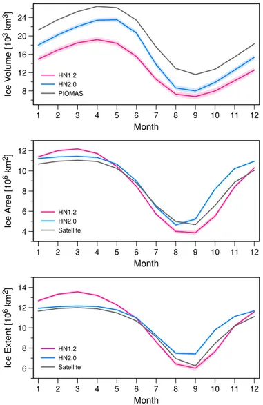
The mean seasonal cycle of sea-ice volume, sea-ice area, and sea-ice extent is shown in Figure3 (sea-ice extent is defined here as the area of all grid cells with more than 15% sea-ice concentration).
The across-ensemble scatter in the mean seasonal cycle of all these variables is generally low.
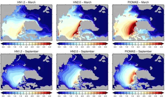
This indicates that the climatological differences between HN1.2 and HN2.0 are robust and statistically reliable. HN2.0 simulates an ice volume which is in all months much closer to the PIOMAS data than those from the HN1.2 simulations, even though the PIOMAS ice volume is still higher throughout the year. Largest differences between HN2.0 and PIOMAS appear in August and September as a result of around 1 m thinner ice in the central Arctic in HN2.0. However, despite thinner ice, the geographical distribution of rather thick and rather thin ice within the Arctic pack ice region in HN2.0 agrees rather well with PIOMAS, representing a clear improvement as compared to HN1.2 (see Figure4).
With respect to ice area and ice extent, HN2.0 shows rather good agreement with the satellite data from January to August. In particular, the considerable and permanent overestimate of sea ice in the Labrador Sea during winter in HN1.2 (Figure4; top left) does not appear in HN2.0 any longer. Instead, sea ice in the Labrador Sea is even slightly underestimated as compared to PIOMAS and satellite data.
In contrast, the ice extent in the Greenland and Barents seas is still overestimated during the cold season, but this bias is reduced as compared to HN1.2.
The agreement between HN2.0 and the satellite data is not as good between September and December. The seasonal increase in ice area and ice extent appears too early and is stronger than in the satellite data. Larger parts of the Kara and Chukchi seas are ice covered in September, and the overestimate of ice area and ice extent persists until December. The early ice growth in the Kara and Chukchi seas is associated with a cold temperature bias in the upper ocean (see also Figure 7;
bottom middle). This cold ocean temperature bias might be one of the reasons for accelerated ice growth and the overestimate of ice area and ice extent until the end of the year. Another reason for this overestimate could be reduced values of the reference thicknesses for lateral freezing as compared to HN1.2 (see TableA3). The original values introduced by Dorn et al. [6] had resulted in generally overestimated sea-ice thickness in HN2.0 and were reduced for that reason. Previous model studies already indicated the important role of the parameterization of lateral freezing in sea-ice models [66–68] and coupled atmosphere-ocean-sea ice models [5,69–71]. Dorn et al. [5] noted that the reference thickness for lateral freezing provides one possibility for tuning a coupled model towards a quasi-realistic state of equilibrium in terms of the ice volume, with the side effect that winter ice concentrations and near-surface air temperatures may be getting worse. For instance, a strong reduction of the ice volume may lead to high ice concentrations and cold near-surface air
temperatures in winter, as it is the case in the current configuration of HN2.0 for all three variables (see also Section3.6). Fine-tuning of the reference thicknesses for lateral freezing might therefore result in a cross-variable bias reduction and is intended as part of generating a new parameter configuration.
8 12 16 20 24
1 2 3 4 5 6 7 8 9 10 11 12
Ice Volume [103 km3]
Month
HN1.2 HN2.0 PIOMAS
4 6 8 10 12
1 2 3 4 5 6 7 8 9 10 11 12
Ice Area [106 km2]
Month
HN1.2 HN2.0 Satellite
6 8 10 12 14
1 2 3 4 5 6 7 8 9 10 11 12
Ice Extent [106 km2]
Month
HN1.2 HN2.0 Satellite
Figure 3.Mean seasonal cycle of sea-ice volume (top), sea-ice area (middle), and sea-ice extent (bottom).
The red lines represent the ensemble mean of the 10-member ensemble of ERAI-driven simulations with HN1.2 and the very narrow red shaded areas the two-standard-deviation range of the ensemble.
Analogously, the blue lines and blue shaded areas represent the HN2.0 ensemble. The gray lines represent sea-ice volume from PIOMAS and sea-ice area and extent from the SMMR and SSM/I-SSMIS satellite data. PIOMAS and satellite data were reduced to the NAOSIM domain. Data voids around the North Pole in the satellite data were filled with distance-weighted averages. All data refer to the period 1979–2014.
HN1.2 − March
0.0 0.5 1.0 1.5 2.0 2.5 3.0 3.5 4.0
HN2.0 − March
0.0 0.5 1.0 1.5 2.0 2.5 3.0 3.5 4.0
PIOMAS − March
0.0 0.5 1.0 1.5 2.0 2.5 3.0 3.5 4.0
HN1.2 − September
0.0 0.5 1.0 1.5 2.0 2.5 3.0 3.5 4.0
HN2.0 − September
0.0 0.5 1.0 1.5 2.0 2.5 3.0 3.5 4.0
PIOMAS − September
0.0 0.5 1.0 1.5 2.0 2.5 3.0 3.5 4.0
Figure 4. Sea-ice thickness climatology (in meters) for March (top) and September (bottom) from ERAI-driven ensemble simulations with HN1.2 (left), ERAI-driven ensemble simulations with HN2.0 (middle), and PIOMAS data (right). PIOMAS data were interpolated to the T-grid of HN2.0. The purple lines represent the climatological 15% sea-ice concentration contour of the respective dataset. Land areas of the T-grid are shown in gray. Note that the T-grids of HN1.2 and HN2.0 slightly differ due to the different horizontal resolution. All data refer to the period 1979–2014.
3.4. Sea-Ice Trends and Variability
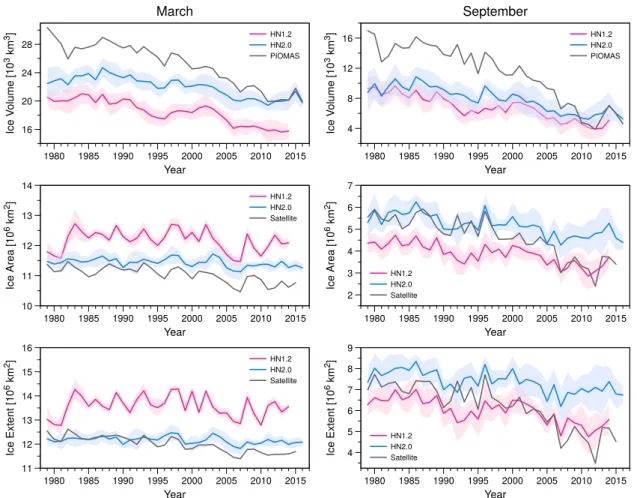
Temporal trends of sea-ice volume, sea-ice area, and sea-ice extent are shown in Figure 5.
The downward trend in the PIOMAS and satellite data is only rudimentarily reproduced by HN1.2 and even still less by HN2.0. However, HN2.0 is close to the PIOMAS ice volume at the end of the simulation period, and shows similarities in ice area and extent with the satellite data in the first half of the simulation period. In contrast, HN1.2 is closer to the satellite data in September ice area and extent at the end of the simulation period. Given that the ocean model uses climatological boundary forcing and that greenhouse gases are constant in the two ensembles, the underestimate of the observed downward trend in sea ice is not a surprise. The existing, but weak downward trend in sea-ice volume, area, and extent in the ensemble simulations can thus only arise from large-scale atmospheric changes entering the model via the atmospheric model boundaries, in combination with internal atmosphere-ocean-ice feedback.
The reason HN1.2 is closer to the satellite data in September ice area and extent at the end of the simulation period is attributable to the simple fact that HN1.2 considerably underestimates the sea-ice volume at the beginning of the seasonal melting period. Therefore, lower melting rates are already sufficient to arrive at low ice area and extent in September similar to the satellite data. Although HN2.0 shows higher melting rates compared to HN1.2 (as can be deduced from the differences of the ice volumes in May and September; see Figure3; top), they are not high enough to reduce the thicker ice cover in HN2.0 to a state similar to the effect of lower melting rates on the thinner ice cover in HN1.2. Since the average melting rate in PIOMAS (3.64·103km3/month) is closer to that in HN2.0 (3.88·103km3/month) than to that in HN1.2 (2.90·103km3/month), HN2.0 also performs better than HN1.2 with regard to the melting rate.
16 20 24 28
1980 1985 1990 1995 2000 2005 2010 2015 Ice Volume [103 km3]
Year
March
HN1.2 HN2.0 PIOMAS
4 8 12 16
1980 1985 1990 1995 2000 2005 2010 2015 Ice Volume [103 km3]
Year
September
HN1.2 HN2.0 PIOMAS
10 11 12 13 14
1980 1985 1990 1995 2000 2005 2010 2015 Ice Area [106 km2]
Year
HN1.2 HN2.0 Satellite
2 3 4 5 6 7
1980 1985 1990 1995 2000 2005 2010 2015 Ice Area [106 km2]
Year
HN1.2 HN2.0 Satellite
11 12 13 14 15 16
1980 1985 1990 1995 2000 2005 2010 2015 Ice Extent [106 km2]
Year
HN1.2 HN2.0 Satellite
4 5 6 7 8 9
1980 1985 1990 1995 2000 2005 2010 2015 Ice Extent [106 km2]
Year
HN1.2 HN2.0 Satellite
Figure 5.Temporal trends of sea-ice volume (top), sea-ice area (middle), and sea-ice extent (bottom) in March (left column) and September (right column) from 1979 to 2016. The red lines represent the ensemble mean of the 10-member ensemble of ERAI-driven simulations with HN1.2 and the red shaded areas the two-standard-deviation range of the ensemble. Analogously, the blue lines and blue shaded areas represent the HN2.0 ensemble. The gray lines represent sea-ice volume from PIOMAS and sea-ice area and extent from the SMMR and SSM/I-SSMIS satellite data. PIOMAS and satellite data were reduced to the NAOSIM domain. Data voids around the North Pole in the satellite data were filled with distance-weighted averages.
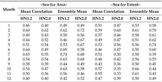
In order to detect coherent variability in the model data and the reference data, it is useful to evaluate the detrended time series. On that account, correlation coefficients between the detrended time series of the PIOMAS and satellite data on the one hand and the model data on the other hand have been calculated. The results are listed in Table2for each month of the detrended ice volume time series and in Table3for each month of the detrended ice area and ice extent time series. With respect to the ice volume, HN2.0 shows significantly higher correlations with the PIOMAS data than HN1.2.
This applies to all months, to the mean correlation of the ensemble members, and to the correlation of the ensemble mean, and clearly indicates an improved year-to-year variability in HN2.0. With respect to ice area and ice extent, H1.2 and HN2.0 show similar correlations with the satellite data, except for the ice extent in the second half of the year (July to December) where HN1.2 shows higher correlations than HN2.0. The latter is associated with the larger sea-ice extent bias in HN2.0 that appears from September to December (see Figure3; bottom) and represents the only major weakness of HN2.0 compared to HN1.2.
Table 2.Correlation coefficients between the detrended monthly time series of the simulated sea-ice volume and the PIOMAS sea-ice volume. The term “Mean correlation” indicates the mean correlation coefficients between PIOMAS and each of the 10 individual ensemble members; the term “Ensemble mean” indicates the correlation coefficients between PIOMAS and the ensemble mean time series.
Month
–Sea-Ice Volume–
Mean Correlation Ensemble Mean HN1.2 HN2.0 HN1.2 HN2.0
1 0.26 0.56 0.31 0.67
2 0.33 0.60 0.39 0.72
3 0.33 0.60 0.39 0.71
4 0.33 0.61 0.38 0.72
5 0.30 0.58 0.35 0.68
6 0.36 0.52 0.42 0.62
7 0.40 0.52 0.48 0.65
8 0.29 0.52 0.35 0.66
9 0.28 0.52 0.34 0.66
10 0.30 0.55 0.36 0.69
11 0.29 0.58 0.36 0.73
12 0.27 0.61 0.32 0.76
Table 3.Like Table2, but for simulated and satellite-derived sea-ice area and sea-ice extent.
Month
–Sea-Ice Area– –Sea-Ice Extent–
Mean Correlation Ensemble Mean Mean Correlation Ensemble Mean HN1.2 HN2.0 HN1.2 HN2.0 HN1.2 HN2.0 HN1.2 HN2.0
1 0.46 0.40 0.49 0.49 0.51 0.47 0.53 0.58
2 0.60 0.62 0.62 0.72 0.59 0.60 0.61 0.70
3 0.49 0.43 0.50 0.56 0.57 0.46 0.58 0.61
4 0.44 0.52 0.46 0.67 0.49 0.47 0.51 0.62
5 0.51 0.54 0.53 0.67 0.53 0.56 0.56 0.74
6 0.64 0.49 0.69 0.58 0.46 0.47 0.50 0.60
7 0.65 0.55 0.74 0.68 0.51 0.30 0.58 0.39
8 0.54 0.54 0.63 0.68 0.48 0.42 0.56 0.55
9 0.38 0.39 0.44 0.49 0.43 0.36 0.50 0.45
10 0.54 0.47 0.63 0.58 0.57 0.35 0.66 0.44
11 0.50 0.36 0.56 0.46 0.55 0.33 0.61 0.43
12 0.40 0.40 0.42 0.52 0.47 0.39 0.50 0.49
In comparison with the low ensemble scatter with respect to the mean seasonal cycle, the ensemble scatter for individual years is relatively large (see also Figure5). The strongest ensemble scatter in ice area and extent appears in the summer months with deviations of up to 1.3·106km2, while the ensemble member deviations in ice volume can amount up to 2.5·103km3 throughout the year.
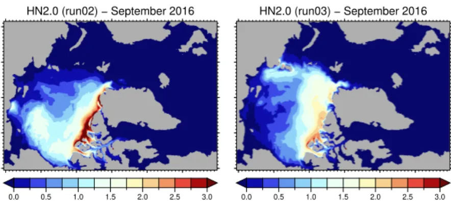
Generally, the scatter in the HN2.0 ensemble is in most years a little larger than in HN1.2. The large ensemble scatter in individual years emphasizes the importance of internally generated variability in the model. Even though the model is constrained at the lateral boundaries, it is able to generate different sea-ice states in its interior with the same forcing from the exterior, as demonstrated in Figure6, which shows the simulated Arctic sea-ice thickness distribution in September 2016 from two ensemble members. Deviations from observed sea-ice conditions in specific years can therefore also be a consequence of internal model variability.
HN2.0 (run02) − September 2016
0.0 0.5 1.0 1.5 2.0 2.5 3.0
HN2.0 (run03) − September 2016
0.0 0.5 1.0 1.5 2.0 2.5 3.0
Figure 6.Mean sea-ice thickness (in meters) in September 2016 from two ensemble members, labeled as run02 (left) and run03 (right), of the ERAI-driven ensemble simulations with HN2.0, as an example for the coupled model’s ability to generate different sea-ice states under identical boundary conditions.
Land areas of the T-grid are shown in gray.
3.5. Upper Ocean Temperatures
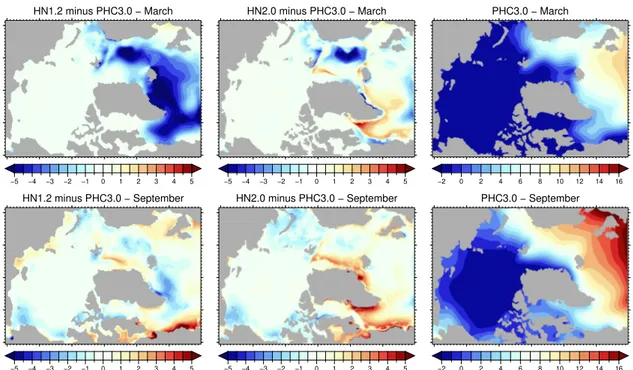
In regions where sea ice is present, the upper ocean temperatures cannot differ widely from the freezing temperature of sea water. Largest temperature biases therefore occur in regions without sea ice or with large sea-ice bias. In March, the upper ocean temperatures in HN1.2 are generally too cold over most of the northern North Atlantic (Figure7; top left). The colder ocean temperatures are in agreement with the overestimate of sea ice in HN1.2, especially in the Labrador Sea. In HN2.0, a similarly strong cold temperature bias appears only in the center of the Nordic Seas (Figure7; top middle).
This temperature bias amounts to around−5◦C and might explain the model’s tendency to extend the sea-ice edge from the Greenland Sea up to the Norwegian Sea. In the Labrador Sea, however, HN2.0 shows warmer ocean temperatures which contribute to an ice-free Labrador Sea. This warm temperature bias in the Labrador Sea also exists in the warm season (Figure7; bottom middle).
The structure of the temperature biases in HN2.0 further indicates that the model tends to direct a relatively larger portion of the warm Atlantic water into the West Spitsbergen Current (leading to warmer temperatures in the Greenland Sea) than into the North Cape Current (leading to colder temperatures in the Barents Sea). This tendency appears throughout the year and might also be responsible for warmer ocean temperatures in the areas of the cold East Greenland Current and the cold East Islandic Current.
Such a behavior is only rudimentarily visible in HN1.2, where the cold ocean temperature bias dominates the cold season. There is a year-round cold bias of more than−2◦C in the Irminger Sea between Iceland and South-East Greenland which spreads into adjacent sea regions further south.
This bias originates from the coupling with HIRHAM and represents a discontinuity compared to the uncoupled part of the domain where the atmospheric forcing comes from ERAI (the same forcing as in HN2.0): the boundary of the coupling domain is clearly visible in HN1.2 with colder ocean temperatures inside the coupling domain compared to slightly warmer temperatures outside.
The discontinuity at the boundary of the coupling domain in HN1.2 appears in other variables as well and represents a general shortcoming of the old coupling procedure. Also for that reason, the coupling procedure has been completely revised for HN2.0, with the result that the atmospheric surface fluxes inside and outside the coupling domain basically agree in their temporal and spatial variation, despite the differences in calculation methods. Consequently, the transition from inside to outside the coupling domain is smooth and the discontinuity does not appear any longer in HN2.0.
This outcome represents an additional improvement compared to the previous model version.
HN1.2 minus PHC3.0 − March
−5 −4 −3 −2 −1 0 1 2 3 4 5
HN2.0 minus PHC3.0 − March
−5 −4 −3 −2 −1 0 1 2 3 4 5
PHC3.0 − March
−2 0 2 4 6 8 10 12 14 16
HN1.2 minus PHC3.0 − September
−5 −4 −3 −2 −1 0 1 2 3 4 5
HN2.0 minus PHC3.0 − September
−5 −4 −3 −2 −1 0 1 2 3 4 5
PHC3.0 − September
−2 0 2 4 6 8 10 12 14 16
Figure 7.Climatological difference in upper ocean temperature (in degrees Celsius) for March (top) and September (bottom) from ERAI-driven ensemble simulations with HN1.2 (left) and ERAI-driven ensemble simulations with HN2.0 (middle). The difference relates to PHC3.0 data (right). Upper ocean refers here to the average over the upper 20 m of the respective ocean data set. PHC3.0 data were interpolated to the T-grid of HN2.0 (and to the T-grid of HN1.2, respectively, for calculating the difference to HN1.2). Land areas of the T-grid are shown in gray. Note that the T-grids of HN1.2 and HN2.0 slightly differ due to the different horizontal resolution. The model data refer to the period 1979–2014.
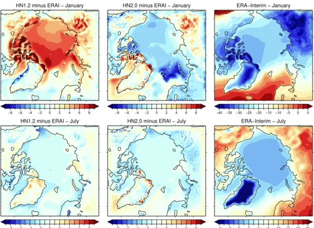
3.6. Near-Surface Air Temperatures 3.6.1. Winter
Wintertime near-surface air temperatures are naturally strongly affected by the surface type, particularly whether the surface is land, ocean, or sea ice. Consequently, the largest winter temperature biases in HN2.0 coincide with the largest biases in sea-ice extent. Figure8(top) shows that the mean January temperatures are 7–8◦C colder over the northern Barents Sea, associated with the overestimate of sea ice in this region, and 5–6◦C warmer over the Labrador Sea, associated with the underestimate of sea ice there. More conspicuous is that HN2.0 shows 2–4◦C colder January temperatures over the ice-covered Arctic Ocean compared to ERAI.
The winter temperature biases in HN1.2 are totally different. On the one hand, the January temperatures are 1–2◦C colder over the Labrador Sea, associated with the permanent overestimate of sea ice in this region, on the other hand, HN1.2 shows 4–8◦C warmer January temperatures over the ice-covered Arctic Ocean as compared to ERAI. This means that there are differences between HN2.0 and HN1.2 of up to 12◦C over sea ice, while temperature differences over land are relatively small (less than 5◦C). Except for the Labrador Sea and the sea region around the southern tip of Greenland, winter temperatures are in HN2.0 colder than in HN1.2. Given that HN2.0 has erroneously used pre-industrial greenhouse gas concentrations, the colder temperatures might be explained to some degree by the associated reduced longwave radiative forcing. However, the warm temperature bias over sea ice in HN1.2 is definitely a major shortcoming of the old model version that does not appear in the new model version. In addition, considering that ERAI has a warm wintertime bias in surface air temperature over Arctic sea ice [62], slightly colder temperatures in HN2.0 represent an improvement compared to the significantly warmer temperatures in HN1.2.
HN1.2 minus ERAI − January
−8 −6 −4 −2 0 2 4 6 8
HN2.0 minus ERAI − January
−8 −6 −4 −2 0 2 4 6 8
ERA−Interim − January
−40 −35 −30 −25 −20 −15 −10 −5 0 5
HN1.2 minus ERAI − July
−8 −6 −4 −2 0 2 4 6 8
HN2.0 minus ERAI − July
−8 −6 −4 −2 0 2 4 6 8
ERA−Interim − July
−6 −3 0 3 6 9 12 15 18 21
Figure 8.Climatological difference in 2-m air temperature (in degrees Celsius) for January (top) and July (bottom) from ERAI-driven ensemble simulations with HN1.2 (left) and ERAI-driven ensemble simulations with HN2.0 (middle). The difference relates to ERAI data (right). ERAI data were interpolated to the HIRHAM5-grid. The black lines represent the coastlines of HIRHAM5, defined as 50% land-sea fraction. All data refer to the period 1979–2014.
3.6.2. Summer
Summertime near-surface air temperatures are usually close to the freezing temperature of water over Arctic sea ice. This holds for the July temperatures in ERAI which are on average a little above 0◦C in the central Arctic (Figure8; bottom). Both HN2.0 and HN1.2 show on average temperatures below 0◦C in this region which are around 1.3◦C colder than ERAI. The reason for that is unclear. It could possibly be associated with the underestimation of sea-ice concentration by about 10% (not shown) and thus more open water area with surface temperatures at the salinity-dependent freezing temperature of sea water (usually between−1.8 and−1.4◦C).
Even though this temperature bias is low, it might have consequences for the way sea ice is melting in the model. Due to the air temperatures being below 0◦C, melting of the snow/ice pack from above is reduced and melt ponds are underrepresented. Instead, sea ice is melting from below through increased heat fluxes entering the upper ocean layer due to the larger open water area.
A restriction of the decrease in sea-ice concentration when melting conditions occur could potentially contribute to reducing both the open water bias and the temperature bias. This will be the subject of forthcoming studies.
Another systematic bias of HN2.0 appears in the boundary zone, where the model overestimates the near-surface air temperatures. The reason for this warm temperature bias is a permanent underestimate of clouds in the boundary zone, in which specific humidity, cloud water, and cloud ice are relaxed to ERAI data. This bias is not a special feature of the coupled model, but appears in HIRHAM5 stand-alone simulations as well. Several efforts have been undertaken to overcome this problem, as for instance different boundary relaxation functions, changes of the boundary zone width, an inflow/outflow formulation for specific humidity, cloud water, and cloud ice at the boundary,
modifications in the cloud parameterization, and others, but the boundary problem has not yet been solved. Only the inflow/outflow formulation helped to restrict the problem to the outermost boundary points.
4. Conclusions and Outlook
The upgraded version of the coupled Arctic atmosphere-ocean-sea ice model HIRHAM–NAOSIM (HN2.0) has been described, and the current base configuration of HN2.0 has been evaluated against observationally based data sets, focusing on sea ice. Compared to the previous version (HN1.2), the upgraded version shows a number of improvements including a generally thicker Arctic sea-ice cover, where the sea-ice thickness distribution is in better agreement with the PIOMAS data set.
Wintertime biases in sea-ice extent, upper ocean temperatures, and near-surface air temperatures are reduced as well, while summertime biases are of similar magnitude as in the previous version.
The revised coupling procedure in HN2.0, which makes use of the coupling software YAC, is highly efficient from a computational point of view and performs flawlessly from a physical point of view. While HN1.2 still shows discontinuities in the upper ocean fields at the boundary of the coupling domain, HN2.0 reveals a rather smooth transition from inside to outside the coupling domain without any discontinuity. It is suggested that this additional improvement in HN2.0 can not only be attributed to improved physical parameterizations in the atmosphere component HIRHAM5 but also to the new coupling procedure, which applies conservative remapping and consistent time averaging of coupling fields. The outcome is that atmospheric surface fluxes inside and outside the coupling domain basically agree in their temporal and spatial variation.
The choice of parameters for the current base configuration of HN2.0 has turned out to be still in need of improvement. A couple of parameter adaptations and their tendential effect on the model results have already been tested in HN2.0; however, as already known from previous work [6], an adequate harmonization of various parameters is needed to reduce model biases. In particular, the mixing ratios of greenhouse gases, the reference thicknesses for lateral freezing of sea ice, and the fractions of snow and melt ponds need to be reassessed and harmonized with other parameters that are not well established by observations. Such a reassessment and harmonization of model parameters is currently in progress and will eventually lead to a revised model configuration that may show an even better performance. The model may also benefit from time-varying lateral ocean boundary forcing based on ocean reanalyses which are envisaged to replace the Levitus climatology.
Moreover, the upgraded version of HIRHAM–NAOSIM has been designed as a tool for advancing our understanding of interaction processes between atmosphere, sea ice, and ocean in combination with observations. Simple fine-tuning of individual parameters/parameterizations towards better model performance is therefore not the primary objective. Instead, more realistic parameterizations should be developed on the basis of observations.
A short-term objective is the implementation of the stability-dependent parameterization of the transfer coeffcients for momentum and heat over sea ice by Lüpkes and Gryanik [72].
This parameterization also includes form drag caused by the edges of ice floes and melt ponds, which is disregarded in the present parameterization. The translation of the new parameterization into the model source code has recently been completed. The first sensitivity studies with respect to this new parameterization are underway. It is anticipated that the additional form drag of the sea ice will lead to improvements in the sea-ice drift.
The inclusion of ice thickness classes in the heat flux calculation of the atmospheric component may be a useful step to improve the thermodynamic coupling between atmosphere and sea ice.
Castro-Morales et al. [73] showed that even a change from seven uniform ice thickness classes (as currently implemented in NAOSIM) to fifteen nonuniform ice thickness classes (derived from field measurements) has the potential to improve the representation of the sea-ice energy balance considerably. Discussions based on how such a nonuniform ice thickness distribution can be implemented in the atmospheric component HIRHAM5 are underway.