Potential sources of variability in mesocosm experiments on the response of phytoplankton to ocean acidiﬁcation

(1)

www.biogeosciences.net/14/1883/2017/

doi:10.5194/bg-14-1883-2017

Potential sources of variability in mesocosm experiments on the response of phytoplankton to ocean acidification

Maria Moreno de Castro¹, Markus Schartau², and Kai Wirtz¹

1Helmholtz-Zentrum Geesthacht, Centre for Materials and Coastal Research, Geesthacht, Germany

2GEOMAR Helmholtz Centre for Ocean Research Kiel, Kiel, Germany

Correspondence to:Maria Moreno de Castro (maria.morenodecastro@outlook.com) Received: 9 March 2016 – Discussion started: 8 April 2016

Revised: 6 March 2017 – Accepted: 13 March 2017 – Published: 6 April 2017

Abstract.Mesocosm experiments on phytoplankton dynamics under high CO₂ concentrations mimic the response of marine primary producers to future ocean acidification. How- ever, potential acidification effects can be hindered by the high standard deviation typically found in the replicates of the same CO₂treatment level. In experiments with multiple unresolved factors and a sub-optimal number of replicates, post-processing statistical inference tools might fail to detect an effect that is present. We propose that in such cases, data-based model analyses might be suitable tools to unearth potential responses to the treatment and identify the uncertainties that could produce the observed variability. As test cases, we used data from two independent mesocosm experiments. Both experiments showed high standard deviations and, according to statistical inference tools, biomass appeared insensitive to changing CO₂conditions. Conversely, our simulations showed earlier and more intense phytoplankton blooms in modeled replicates at high CO₂concentrations and suggested that uncertainties in average cell size, phytoplankton biomass losses, and initial nutrient concentration potentially outweigh acidification effects by triggering strong variability during the bloom phase. We also estimated the thresholds below which uncertainties do not escalate to high variability. This information might help in designing future mesocosm experiments and interpreting controversial results on the effect of acidification or other pressures on ecosystem functions.

1 Introduction

Oceans are a sink for about 30 % of the excess atmospheric CO2generated by human activities (Sabine et al., 2004). In- creasing carbon dioxide concentration in aquatic environ- ments alters the balance of chemical reactions and thereby produces acidity, which is known as ocean acidification (OA) (Caldeira and Wickett, 2003). Interestingly, the sensitivity of photoautotrophic production of particulate organic carbon (POC) to OA is less pronounced than previously thought.

Several studies on CO₂ enrichment revealed an overall increase in POC (e.g., Schluter et al., 2014; Eggers et al., 2014;

Zondervan et al., 2001; Riebesell et al., 2000), but other studies did not detect CO₂effects on POC concentration (e.g., Jones et al., 2014; Engel et al., 2014) or primary production (Nagelkerken and Connell, 2015). General compilation studies that document controversial results are, e.g., Riebe- sell and Tortell (2011) and Gao et al. (2012).

In some experiments, the different treatment levels, i.e., different CO2concentrations, have been applied in parallel repetitions, also known as replicates or sample units. This was the case in several CO2perturbation experiments with mesocosms (Riebesell et al., 2008). Often, high variances are found in measurements among replicates of similar CO₂levels (Paul et al., 2015; Schulz et al., 2008; Engel et al., 2008;

Kim et al., 2006; Engel et al., 2005). It is this variance in data that reflects system variability, thereby introducing a severe reduction in the ratio between a true acidification response signal and the variability in observations. Ultimately, the experimental data exhibit a low signal-to-noise ratio.

Mesocosms typically enclose natural plankton communi- ties, which is a more realistic experimental setup compared to

(2)

batch or chemostat experiments with monocultures (Riebe- sell et al., 2008). Along with this, mesocosms allow for a larger number of possible planktonic interactions that provide opportunities for the spread of uncontrolled heterogene- ity. Moreover, physiological states vary for different phytoplankton cells and environmental conditions. For this reason, independent experimental studies at similar but not identical conditions might yield divergent results. The variability in data of mesocosm experiments is thus generated by variations of ecological details, i.e., small differences among replicates of the same sample, such as in species abundance, nutrient concentration, and metabolic states of the algae at the initial setup of the experiments. Differences of these factors often remain unresolved and might therefore be treated as uncertainties in a probabilistic approach.

To account for all possible factors that determine all differences in plankton dynamics is practically infeasible, which also impedes a retrospective statistical analysis of the experimental data. However, since unresolved ecological details might propagate over the course of the experiment, it is meaningful to consider a dynamical model approach to up- grade the data analysis. From a modeling perspective, some important unresolved factors translate into (i) uncertainties in specifying initial conditions (of the state variables), and (ii) uncertainties in identifying model parameter values. Here, we apply a dynamical model to estimate the effects of ecophysiological uncertainties on the variability in POC concentration of two mesocosm experiments. Our model describes plankton growth in conjunction with a dependency between CO2utilization and mean logarithmic cell size (Wirtz, 2011).

The structure of our model is kept simple, thereby reducing the possibility of overparameterizing the mesocosms dynamics. The model is applied to examine how uncertainties in individual factors, namely initial conditions and parameters, can produce the standard deviation of the distribution of observed replicate data. Our main working hypotheses on the origins of variability in mesocosm experiments are the following:

– Differences among replicates of the same sample can be interpreted as unresolved random variations (named uncertainties hereafter).

– Uncertainties can amplify during the experiment and generate considerable variability in the response to a given treatment level.

– Which uncertainties are more relevant can be estimated by the decomposition of the variability in the experimental data.

For our data-supported model analysis of variability decomposition we consider the propagation of distributions (JCGM, 2008b) to seek potential treatment responses that are masked by the variability in observations of two independent OA mesocosm experiments, namely, the Pelagic Enrich- ment CO₂Experiment (PeECE II and III). The central idea

is to produce ensembles of model simulations, starting from a range of values for selected factors. The range of values for these selected factors is determined so as the variability in model outputs does not exceed variability in observations over the course of the experiment. The margins of the variational range of each factor were thus confined by the ability of the dynamical model to reproduce the magnitude of the variability observed in POC. These confidence intervals describe the tolerance thresholds below which uncertainties do not escalate to high variability in the modeled replicates, and can serve as an estimator of the tolerance of experimental replicates to such uncertainties. This information can be important to ensure reproducibility, allowing for a comparison between the results of different independent experiments and increasing confidence regarding the effects of OA on phytoplankton (Broadgate et al., 2013).

2 Method

Potential sources of variability are estimated following a procedure already applied in system dynamics, experimental physics, and engineering (JCGM, 2008b). The basic principles of uncertainty propagation are summarized here using a six-step method (see Fig. 1). Steps 1 and 2 are described in Sect. 2.1 and comprise a classical model calibration (using experimental data of biomass and nutrients) to obtain the reference run representing the mean dynamics of each treatment level. In this way we found the reference value for the model factors, i.e., parameters and initial conditions. Steps 3 and 4, described in Sect. 2.2, include the tracked propagation of uncertainties by systematically creating model trajectories for POC, each one with a slightly different value of a model factor. In steps 5 and 6, we estimated the thresholds of the model-generated variability and the effect of the uncertainty propagation (also explained in Sect. 2.2).

2.1 Model setup, data integration, and description of the reference run

In this section, we describe the biological state that was used as reference dynamics. Our model resolves a minimal set of state variables insofar monitored during experiments that are assumed to be key agents of the biological dynamics. Model equations are shown in Table 1. Reference values of the parameters are shown in Table 2. An exhaustive model docu- mentation is given in Appendix A. The model simulates experimental data from the Pelagic Enrichment CO₂ Experi- ment (PeECE), a set of nine outdoor mesocosms placed in coastal waters close to Bergen (Norway) during the spring seasons of 2003 (PeECE II) and 2005 (PeECE III). In both the experiments, blooms of the natural phytoplankton community were induced and treated in three replicates for the future, present, and past CO₂conditions (Engel et al., 2008;

Schulz et al., 2008; Riebesell et al., 2007, 2008). Experimen-

(3)

Table 1.States variables and their dynamics.

State variable Dynamical equation Ini. cond. Units

Phytoplankton carbon ^dPhy_dt^C=(P−R−L)·Phy_C 2.5 µmol-C L⁻¹ Phytoplankton nitrogen ^dPhy_dt^N =V·Phy_C−L·Phy_N 0.4 µmol-N L⁻¹ Nutrient concentration ^dDIN_dt =r·DH_N−V·Phy_C 8±0.5^∗ µmol-N L⁻¹ 14±2^∗∗ µmol-N L⁻¹ Detritus and heterotrophs C ^dDH_dt^C =L·Phy_C−(s·DH_C+r)·DH_C 0.1 µmol-C L⁻¹ Detritus and heterotrophs N ^dDH_dt^N =L·Phy_N−(s·DHN+r)·DHN 0.01 µmol-N L⁻¹

∗PeECE II,^∗∗PeECE III

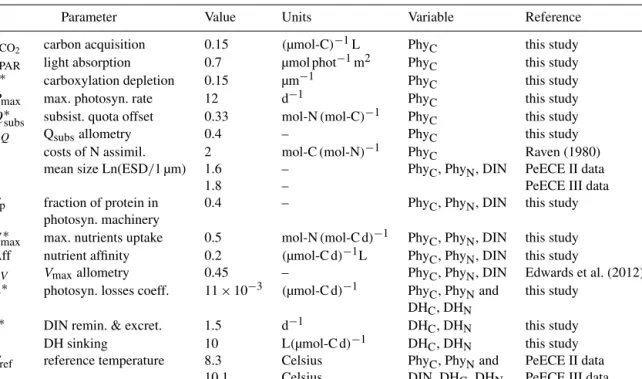
Table 2.Parameter values used for the reference run,hφ_ii. All values are common to both PeECE II and III experiments, only the mean temperature (determined by environmental forcing) and the averaged cell size in the community are different since different species composition succeeded in the experiments (Emiliania huxleyiwas the major contributor to POC in PeECE II (Engel et al., 2008) but also diatoms significantly bloomed during PeECE III (Schulz et al., 2008).

Parameter Value Units Variable Reference

a_CO₂ carbon acquisition 0.15 (µmol-C)⁻¹L Phy_C this study

a_PAR light absorption 0.7 µmol phot⁻¹m² Phy_C this study

a^∗ carboxylation depletion 0.15 µm⁻¹ Phy_C this study

Pmax max. photosyn. rate 12 d⁻¹ Phy_C this study

Q^∗_subs subsist. quota offset 0.33 mol-N(mol-C)⁻¹ Phy_C this study

α_Q Q_subsallometry 0.4 – Phy_C this study

ζ costs of N assimil. 2 mol-C(mol-N)⁻¹ Phy_C Raven (1980)

` mean size Ln(ESD/1 µm) 1.6 – Phy_C, Phy_N, DIN PeECE II data

1.8 – PeECE III data

fp fraction of protein in 0.4 – Phy_C, Phy_N, DIN this study

photosyn. machinery

V_max^∗ max. nutrients uptake 0.5 mol-N(mol-C d)⁻¹ Phy_C, Phy_N, DIN this study Aff nutrient affinity 0.2 (µmol-C d)⁻¹L Phy_C, Phy_N, DIN this study

α_V Vmaxallometry 0.45 – Phy_C, Phy_N, DIN Edwards et al. (2012)

L^∗ photosyn. losses coeff. 11×10⁻³ (µmol-C d)⁻¹ Phy_C, Phy_Nand this study DH_C, DH_N

r^∗ DIN remin. & excret. 1.5 d⁻¹ DH_C, DH_N this study

s DH sinking 10 L(µmol-C d)⁻¹ DH_C, DH_N this study

T_ref reference temperature 8.3 Celsius Phy_C, Phy_Nand PeECE II data

10.1 Celsius DIN, DH_C, DH_N PeECE III data

tal data are available via the data portal Pangaea (PeECE II team, 2003; PeECE III team, 2005).

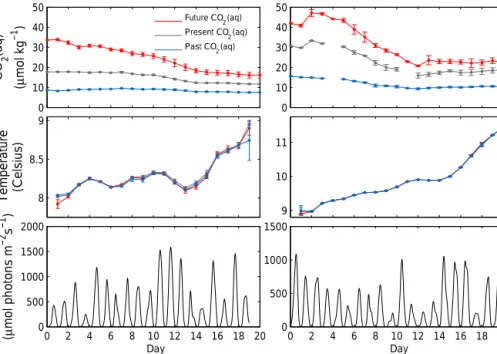
Field data of aquatic CO₂concentration, temperature, and light were used as direct model inputs (see Appendix B).

Measurements of POC, particulate organic nitrogen (PON), and dissolved inorganic nitrogen (DIN) were used for model calibration. Although both the experiments differ in their species composition, environmental conditions, and nutrient supply, the same parameter set was used to fit PON, POC, and DIN from PeECE II and III (i.e., a total of 54 series of repeated measures over more than two weeks), a feature indicating the model skills. In addition, the model

was validated with another 36 series of biomass and nutrients data from an independent mesocosm experiment ((Paul et al., 2014), data not shown). The experimental POC and PON data were redefined for a direct comparison with model results (see Appendix C), since some contributions (e.g., polysaccharides and transparent exopolymer particles) remain unresolved by our dynamical equations. State variables of our model comprise carbon and nitrogen contents of phytoplankton, Phy_C and Phy_N, and DIN, as representative for all nutrients. The dynamics of non-phytoplanktonic components, i.e., detritus and heterotrophs (DH), are distinguished

(4)

Factor mean (from ref. run)

Frequency

Factor values

Step 4:

POC standard deviation

Frequency

POC at a given day Day

Step 1:

model calibration

Model-data fit using biomass and nutrients data (POC, PON and DIN) from 2 mesocosm experiments with

3 treatment levels × 3 replicates

day Step 2:

reference run per treatment

level

Parameter set minimizing model-data residuals:

DIN POC

Step 3:

factor standard deviation

Step 5:

tolerance of mesocosms to

uncertainty

Step 6:

sensitivity coefficient

Estimated by the uncertainty such that simulated POC standard deviation do not exceed

experimental POC standard deviation Concentration day

For each factor:

Virtual replicates for that factor:

Concentration

day PON

Uncertainty

Variability

Residuals Model ref. run

.

Sample mean

= Uncertainty Variability POC

Figure 1.Variability decomposition method based on uncertainty propagation (summary of the basic principles given in Sect. 5.1.1 and 5.6.2. and Annex B in JCGM, 2008b).

by DH_Cand DH_N. Thus, in our study, POC=Phy_C+DH_C and PON=Phy_N+DH_N.

The mean cell size in the community, represented as the logarithm of the mean equivalent spherical diameter (ESD), was used as a model parameter. It determines specific ecophysiological features by using allometric relations that are relevant for the computation of subsistence quota, as well as nutrient and carbon uptake rates. Regarding the latter, to resolve sensitivities to different DIC conditions, we used a relatively accurate description of carbon acquisition as a function of DIC and size. It has been suggested by previous observations and models that ambient DIC concentration increases primary production (e.g., Schluter et al., 2014; Rost et al., 2003; Zondervan et al., 2001; Riebesell et al., 2000; Chen, 1994; Riebesell et al., 1993; Riebesell and Tortell, 2011) and mean cell size in the community (Sommer et al., 2015; Eg- gers et al., 2014; Tortell et al., 2008). While state-of-the-art models such as Artioli et al. (2014) used empirical biomass increase to describe OA effects, we adopted and simplified a biophysically explicit description for carbon uptake from Wirtz (2011), where the efficiency of intracellular DIC trans- port has been derived as a function of the mean cell size

`=ln(ESD/1 µm) and CO₂ concentration. For very large

cells, the formulation converges to the surface to volume ratio, which in our notation reads e^−`. In contrast, the dependence of primary production on CO₂vanishes for (does not apply to) picophytoplankton; the rate limitation by sub- optimal carboxylation then reads

fCO₂ = 1−e^−a^CO2^·CO² 1+a^∗·e^(`−a^CO2^·CO²⁾

!

. (1)

The specific carbon absorption coefficientaCO₂ reflects size- independent features of the DIC acquisition machinery (for instance, the carbon concentration mechanisms, Raven and Beardall, 2003). The coefficient a^∗represents carboxylation depletion.

2.2 Uncertainty propagation

We considered that uncertainties were only present in the initial setup of the system; this allowed us to perform a deterministic non-intrusive forward propagation of uncertainty, which neglects the possible coupling between uncertainties and temporal dynamics unlike in intrusive methods (Chantrasmi and Iaccarino, 2012) involving stochastic dynamical equations with time-varying uncertainties (Toral and Colet, 2014; de Castro, 2017. Forward refers to the fact that unresolved differences among replicates simulated as variations of the model control factors are propagated through the model to project the overall variability in the system response, in contrast to backward methods of parameter estimation where the likelihood of input values is conditioned by the prior knowledge of the output distribution (as, for instance, in Larssen et al., 2006).

Our approach is based on a Monte Carlo method for the propagation of distributions. It is based on the repeated sampling from the distribution for possible inputs and the evalu- ation of the model output in each case (JCGM, 2008b). Next, the overall simulated POC variability is compared with that in POC experimental data (i.e., the mean trends of the treatment levels as well as the standard deviations are compared, the former for the calculation of the reference run and the latter for the uncertainty propagation). Among the available experimental data, we favored POC over PON and DIN in the uncertainty propagation analysis since it is usually the target variable of OA effects and shows the highest variability.

A variability decomposition with more than one dependent variable (equivalent to a multivariate ANOVA design, for instance) is beyond of the scope of the study. The comparison between simulated and experimental variability in POC helps in the identification of the changes in physiological state and community structure that are the main potential contributors to the variability.

We considered model factors,φ_i, withi=1, . . ., N=19, consisting of 14 process parameters and 5 initial conditions for the state variables. Their reference values, hφ_ii, were adjusted to yield model solutions reproducing the mean of

(5)

each treatment level (steps 1 and 2, Tables 1 and 2). To test our first hypothesis, factor variations representing potential uncertainties are introduced as random values distributed around hφ_iiwith standard deviation4φ_i. To calculate4φ_i, we first generate 10⁴simulations, each one with a different factor value,φ_i (steps 3 and 4). The ensemble of model solutions for each factor and treatment level simulates the potential experimental outcomes, hereafter referred to as “virtual replicates”, (see Appendix D). The factor value for each POC trajectory is randomly drawn from a normal distribution around the factor reference valuehφ_ii(same distribution is assumed by popular parametric statistical inference tools such as regressions and ANOVA, Field et al., 2008). For every treatment level and at every time step, we calculated the ensemble average of the virtual replicates,hPOC^mod_i i, and the standard deviation,4POC^mod_i . Thus,4φi is the standard deviation of the distribution of factor values, such as4POC^mod_i , which do not exceed the standard deviation of the experimental POC data,4POC^exp, for any mesocosm at any given time (step 5). The effect of variations ofφ_i on the variability (step 6) is given as follows:

ε_i=4POC^mod_i

4φ_i . (2)

This ratio expresses the maximum variability a factor can generate, 4POC^mod_i , relative to the associated range of that factor variations,4φ_i, to ensure that4POC^mod_i is the closest to4POC^expat any time. In general,ε_i defines how much of the uncertainty of a dependent variable Y (hereY =POC) is explained by and the uncertainty of the input factors φ_i, a proxy of which is known as the sensitivity coefficient ci= ^∂Y

∂φ_i in the widespread formula to calculate error propagation (Ellison and Williams, 2012), also known as law of propagation of uncertainty (JCGM, 2008a)

(4Y )²=

N

X

i=1

c²_i ·(4φ_i)². (3) This expression is based on the assumption that changes in Y in response to variations in one factor φ_i are independent from those owing to changes in another factor φ_j, and that all changes are small (thus cross-terms and higher- order derivatives are neglected). Where no reliable mathe- matical description of the relationship Y (φi)exists (in our case, only an expression for the rate equation dPOC/dt is known (see Table 1) but not its analytical solution, i.e., POC), ci can be evaluated experimentally (Ellison and Williams, 2012; JCGM, 2008a). As mentioned in the Introduction and Appendix A, such high-dimensional multi-factorial measurements are costly in mesocosm experiments. Therefore, we obtained equivalent information by numerically calculating ε_i. Such approximations to sensitivity coefficients calculated by our Monte Carlo method of uncertainty propagation cor- respond to taking all higher-order terms in the Taylor series expansion into account since no linearization is required

(see Sect. 5.10 and 5.11 and Annex B in JCGM, 2008b). A straightforward extension including the cross-terms showing synergistic uncertainties effects, as in an experimental multi- way ANOVA design, requires the assumption of joint distributions for the uncertainty of factors and the calculation of covariance matrices, a considerable effort that is beyond of the scope of this paper.

Hereafter, the standard deviation of any given factor, i.e., factor uncertainty, will be given as percentage of the reference values and will be called48_i. The actual factor range is given as4φ_i=⁴⁸ⁱ^·φⁱ

100 . Strong irregularities in the standard deviations of experimental POC data (for instance, small 4POC^exp at day 8 in Fig. 2p), translates to remarkably en- hanced or reduced sensitivity coefficients if the model–data comparison would be performed at a daily basis. Therefore, we considered the temporal mean of the standard deviation per phase, i.e., prebloom, bloom, and postbloom. We inferred phases for PeECE II from Engel et al. (2008) and for PeECE III from Schulz et al. (2008) and Tanaka et al. (2008).

To numerically calculate the ensemble of 10⁴ POC trajectories per factor (i.e., the virtual replicates; see Fig. 8), we applied the Heun integration method with a time step of 4×10⁻⁴, (about 35 s of experimental time). The number of simulated POC time series is chosen such as a higher number of model realizations, i.e., a higher number of virtual replicates will produce the same results (see Adaptive Monte Carlo procedure, Sect. 7.9. in JCGM, 2008b). We dismissed the negative values that randomly appeared when drawing 10⁴values from the normal distribution of factor values; this reduction in the number of trajectories did not affect the results.

Environmental data showed low variability among similar treatment replicates, (see Fig. 9), suggesting a non-direct relation between variations in environmental factors among replicates and the observed biomass variability. Therefore, we focused on uncertainties in ecophysiology and community composition and used environmental data as forcing.

Perturbations of the similarity among replicates produced by strong changes in environmental conditions (storms, dys- functional devices, etc.) or by errors in manipulation or sampling procedures are not within the scope of this work. Af- ter a few decades, the current state-of-the-art of experimental techniques for running plankton mesocosms is advanced. We believe such differences are of low impact or well understood in terms of their consequences for final outcomes (Riebesell et al., 2010; Cornwall and Hurd, 2015).

Notably, our analysis suggested sufficient (but not necessary; Brennan, 2012) causes of uncertainties in mesocosm experiments. Variations in model characterization including structural variability (Adamson and Morozov, 2014; Fuss- mann and Blasius, 2005) or uncertainties in model parame- terization (Kennedy and O’Hagan, 2001) or comparisons to different uncertainty propagation methods (de Castro, 2017) require further extensive analyses, which is beyond the scope of this study. However, we performed a series of preceding

(6)

0 3 6

PON (µmol−N L⁻¹)

(a)

0 20 40

POC (µmol−C L⁻¹)

(b)

0 5 10

DIN (µmol−N L⁻¹)

(c) F uture CO (aq)₂

0 3 6

(d)

0 20 40

(e)

0 5

10 (f) Present CO (aq)₂

2 4 6 8 10 12 14 16 18 0

3 6

Day

(g)

2 4 6 8 10 12 14 16 18 0

20 40

Day

(h)

2 4 6 8 10 12 14 16 18 0

5 10

Day

(i) Past CO (aq)₂

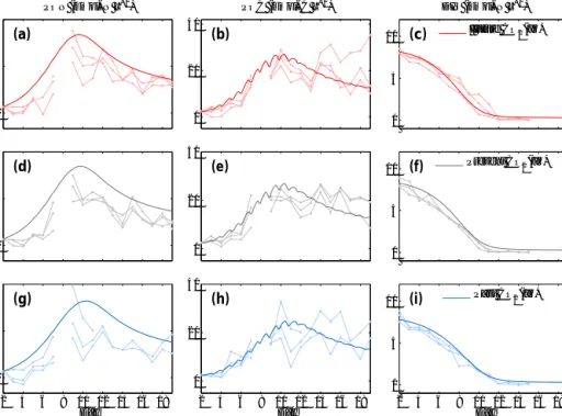
Figure 2.Solid lines show reference runs for POC, PON, and DIN simulating the mean of the replicates per treatment level, with different colors for the three experimental CO₂setups. Dots are replicated data from the Pelagic Enrichment CO₂Experiment (PeECE II) for newly produced POC and PON, i.e., starting values at day 2 were subtracted from subsequent measurements as in Riebesell et al. (2007).

model analyses (including uncertainty propagation) by using slightly different model formulations (data not shown). From these preceding analyses, we found that different model formulations can lead to quantitatively different confidence intervals, but leave the final results qualitatively unchanged.

3 Results

3.1 CO2effect on POC dynamics

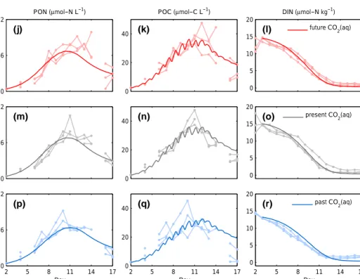
Our model reproduces the means of PON, POC, and DIN experimental data per treatment level, i.e., for the future, present, and past CO₂conditions, in two independent PeECE experiments (Figs. 2 and 3). For PeECE II, PON is moder- ately overestimated and postbloom POC is slightly underes- timated. Nonetheless, the model represents the experimental data with similar precision than the means of experimental replicates (see Appendix E). The means of the same treatment replicates and their associated standard deviations are typically used to represent experimental data (see Fig. 1b in Engel et al., 2008 for PeECE II or Fig. 8a in Schulz et al., 2008 for PeECE III). The means are in the foundations of the statistical inference tools that did not detect acidification responses for PeECE II and III. However, with our mechanis- tic model-based analysis, phytoplankton growth in the future CO₂ conditions showed an earlier and elevated bloom with respect to past CO₂conditions. The future and past reference trajectories limit the range of the CO₂enrichment effect, as

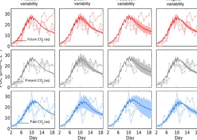
shown by the dark gray area in Fig. 4. POC variability owing to variations in model factors simulating experimental uncertainties is plotted as the light gray area in the figure. Our results suggest that avoiding high POC standard deviations that potentially mask OA effects in experimental data requires the reduction of the factor variations triggering variability during the bloom.

3.2 CO₂effect on uncertainty propagation

The estimation of the tolerance thresholds of the dynamics to uncertainty propagation for the two test-case experiments, per acidification levels and per factor uncertainty, are listed in Table 3. We investigated the potential interaction of the treatment and the uncertainty effects on the tolerance by a linear mixed-effects model withφi as the random factor (R Core Team, 2016). The synergistic effect between the factor uncertainty and the treatment levels was found to be non- significant (F =2.9 withp=0.06). Therefore, the thresholds do not appear to statistically depend on the treatment level, even when the standard deviation of the measured POC data,4POC^exp, for the future and past acidification conditions were, on average, about 70 % larger than the standard deviation of the present conditions (POC experimental data in Figs. 2 and 3 are more spread in the future and past concentrations than in the present concentration). Despite the low statistical power of this test (only data from two independent samples, the two PeECE experiments, were available),

(7)

Table 3.Tolerance of mesocosms experiments to differences among replicates, given as a percentage of the reference factor value listed in Tables 1 and 2. According to our model projections, above these thresholds the simulated variability,4POC^mod_i , exceeds the observed variability,4POC^exp. Main contributors to the simulated variability during the bloom are highlighted in bold (see Sect. 3).

Factorφ_i 48_i(%) Averaged

PeECE II PeECE III tolerance

Future Present Past Future Present Past (%)

Phy_C(0) initial phyto C biomass 68 49 46 78 60 100 67±6

Phy_N(0) initial phyto N biomass 26 19 22 21 16 29 22±4

DIN(0) initial DIN 20 28 29 17 11 18 20±6

a_CO₂ carbon acquisition 89 46 23 86 63 46 59±23

a_PAR light absorption >100 >100 98 >100 >100 92 >100

P_max maximum photosyn. rate 27 18 16 22 16 28 21±5

Q^∗_subs subsistence quota offset 6 5 6 5 4 9 6±1

α_Q Q_subsallometry 9 7 8 7 5 10 8±2

` size Ln(ESD/1µm) 25 20 29 19 14 22 22±5

fp fraction of protein in 92 75 44 36 17 38 50±25

photosyn. machinery

V_max^∗ maximum nutrient uptake 13 11 14 10 8 14 12±2

Aff nutrients affinity 39 31 42 38 36 55 40±7

α_V V_maxallometry 14 11 15 10 8 14 12±2

L^∗ phytoplankton losses 22 30 28 12 10 15 20±8

r^∗ DIN remineralization 73 99 98 128 37 52 81±31

s DH sinking >100 >100 96 >100 61 79 >100

T_ref reference temperature 17 12 14 9 7 14 12±3

0 6 12

PON (µmol−N L⁻¹)

(j)

0 20 40

POC (µmol−C L⁻¹)

(k)

0 5 10 15 20

DIN (µmol−N kg⁻¹)

(l) ^{future CO}2(aq)

0 6 12

(m)

0 20 40 (n)

0 5 10 15 20

(o) ^{present CO}2(aq)

2 5 8 11 14 17

0 6 12

Day

(p)

2 5 8 11 14 17

0 20 40

Day

(q)

2 5 8 11 14 17

0 5 10 15 20

Day

(r) ^{past CO}2(aq)

Figure 3.As in Fig. 2 for PeECE III.

(8)

Figure 4.Reference simulations of POC for high CO₂(red) and low CO₂(blue) conditions bind the range of acidification effect (dark gray) according to our model projections. Light gray area shows the limits of the overall simulated POC variability, 4POC^mod. Inlay graph display the signal-to-noise ration (black solid lines), i.e., the ratio between the variance of the acidification effect and the variance of the overall variability.

we still considered the potential lack of CO₂ effect on the uncertainty propagation as sufficient justification to simplify further analysis on variability decomposition by averaging the thresholds and the sensitivity coefficients over treatment levels (see last column in Table 3 and Fig. 7).

3.3 Variability decomposition

Our method allows for decomposition of POC variability in factor-specific components 4POC^mod_i . The effect of factor variations simulating experimental differences among replicates is classified depending on its nature, intensity, and timing (Figs. 5, 6, and 7).

POC variability during the prebloom phase can be explained mainly by the differences of factors related to subsistence quota, i.e.,Q^∗_subsandα_Q, in both PeECE II and III experiments (left column in Figs. 5 and 6). This suggests that the differences in subsistence quota first intensify the divergence of POC trajectories and then weaken a few days later because of the system dynamics. These subsistence parameters only need to vary about 6 and 8 % among replicates (see Table 3) to maximize their contribution to the4POC^exp; thus, their sensitivity coefficients are the highest (see Fig. 7).

Differences in the initial nutrient concentration, DIN(0), mean cell size, `, and phytoplankton biomass loss coefficient,L^∗, generate the modeled variability mainly during the bloom (with just about 20 % differences among replicates;

see Table 3 and second column in Fig. 5) showing high values of the sensitivity coefficient (highlighted in Fig. 7).

Amplified variability in the postbloom phase (third column in Figs. 5 and 6) can be attributed to the uncertainties

in the reference temperatureTreffor the Arrhenius equation, Eq. (A4), in sinking loss or export flux,s, and in remineralization and excretion,r^∗. The sensitivity coefficient of Tref

is high, with just about 12 % variation. Therefore, even if differences in ambient temperature among replicates of the same sample are negligible (see the low standard deviations in the temperature, Fig. 9), differences in the metabolic dependence on that ambient temperature seems to be relevant in the decay phase. Interestingly, variations among replicates in the physiological dependence on other environmental factors do not show the same relevance (the sensitivity coefficient ε_i is low for carbon acquisition aCO₂ and light absorption aPAR). Generating high divergence during the postbloom requires a strong perturbation of parameters for the description of the non-phytoplanktonic biomass (about 81 % of the reference value for sinking and 96 % for remineralization and excretion, see Table 3), which translates to a relatively low sensitivity coefficient.

Perturbations of the initial detritus concentration, DH_C(0) and DH_N(0)have no impact on the dynamics provided that they remain within reasonable ranges (48_i<100). In fact, more than 10-fold difference among replicates in such non- relevant factors were necessary to achieve a perceptible vari- ability4POC^mod_i .

POC variability throughout the bloom phases (right column in Figs. 5 and 6) can be attributed to the varying carbon and nitrogen initial conditions, Phy_Cand Phy_N, nutrient uptake-related factors,V_max^∗ ,αV, and Aff, and protein allocation for photosynthetic machinery,fp. With regard to the latter, high standard deviations of the tolerance (see Table 3) suggest non-conclusive results.

4 Discussion

We used the uncertainty quantification method to decom- pose POC variability by using a low-complexity model that describes the major features of phytoplankton growth dynamics. The model fits the mean of mesocosm experimental PeECE II and III data with high accuracy for all CO₂treatment levels. We confirmed the working hypotheses (Figs. 5–

7); in particular, we showed that small differences in initial nutrient concentration, mean cell size, and phytoplankton biomass losses are sufficient to generate the experimentally observed bloom variability4POC^exp that potentially mask acidification effects, as discussed in the following subsec- tions.

The results of our analyses are conditioned by the dynamical model equations imposed. Deliberately, the model’s complexity is kept low, mainly to limit the generation of structural errors with respect to model design. At the same time, the level of complexity resolved by the model suffices to explain POC measurements of two independent mesocosm experiments with identical parameter values (see Table 2), which highlights model skill. The used equations comply

(9)

0 10 20 30

F uture CO (aq)₂

0 10 20 30

POC (µmol−C L−1 )

Present CO (aq)₂

2 6 10 14 18

0 10 20 30

D ay

Past CO (aq)₂

2 6 10 14 18

D ay

Postbloom

2 6 10 14 18

D ay

2 6 10 14 18

D ay

variability variabiliy variability

Irregular variability Bloom

Prebloom

Figure 5.POC variability decomposition per factor,4POC^mod_i for PeECE II. Shaded areas are limited by the standard deviation of 10⁴ simulated POC time series (see Sect. 2), around the mean trajectory of the ensemble (solid line). The timing of the amplification of the variability determines four separated kinds of behavior: factor uncertainties generating variability during the prebloom, bloom, postbloom, or at irregular phase (see Sect. 3).

with theories of phytoplankton growth (e.g., Droop, 1973;

Aksnes and Egge, 1991; Pahlow, 2005; Edwards et al., 2012;

Litchman et al., 2007; Wirtz, 2011). The uncertainty propagation employed here can be applied to any model. As long as the model features a similar structural complexity and is also able to reproduce POC with sufficient accuracy, we expect similar qualitative findings with respect to the factors (8_i) and similar identification of the major contributors to the variability. However, we would not expect other models to reveal exactly similar values in the ratio_i, which would likely depend on the equations used to resolve some of the ecophysiological details.

4.1 Nutrient concentration

Differences among replicates in the initial nutrient concentration substantially contribute to POC variability, a sensitivity that is, interestingly, not well expressed when varying the initial cellular carbon or nitrogen content of the algae, Phy_C(0)and Phy_N(0). The relevance of accuracy for the initial nutrient concentration in replicated mesocosms has already been pointed out in Riebesell et al. (2008). Under a constant growth rate, DIN(0) determines the timing of nu-

trient depletion; therefore, differences in the initial nutrient concentration might also translate into temporal variations in the succession of species. We showed that such dependence is noted even in more general dynamics, and that our method can also estimate the variational range for differences in the initial DIN concentration for experiments with a low number of replicates. The standard deviation of DIN(0) in the experimental setup for PeECE III was 50 % of the mean, which is significantly above our tolerance threshold (see Table 3 for initial DIN concentration). Following Riebesell et al. (2007), we considered day 2 as the initial condition, when the measured DIN was 14±2 µmol-C L⁻¹, as shown in Table 1. Since 2 µmol-C L⁻¹ is approximately 14 % of 14 µmol-C L⁻¹, the variability of replicates at day 2 was about 14 %. Therefore, experimental differences in the initial nutrient concentration were similar to the tolerance threshold for the initial DIN established to avoid high variability ((20±6)% in Table 3), which represents an explanation for the high divergence observed in POC measurements.

For PeECE II, experimentally measured DIN concentration at day 0 was 10.7±0.8 µmol-C L⁻¹, suggesting a 7.5 % difference among replicates, which was below our projected tolerance level (7.5 is out of the range[14,26]). The same

(10)

0 20 40

F uture CO (aq)₂

0 20 40

POC (µmol−C L−1 )

Present CO (aq)₂

2 6 10 14

0 20 40

D ay

Past CO (aq)₂

2 6 10 14

D ay

2 6 10 14

D ay

2 6 10 14

D ay Figure 6.As Fig. 5, for PeECE III.

0 5 10 15 20 25 30 35 40 45 PeECE III PeECE II

Pre- bloom post-

Figure 7.Sensitivity coefficients (ε_i; Eq. 2) of factorsφ_i listed in Tables 1 and 2 for different bloom phases in two OA-independent mesocosm experiments. Factors whose uncertainties potentially mask acidification effects (Fig. 4) by triggering variability during the bloom (Figs. 5 and 6) are highlighted.

was noted for day 2, with DIN concentration equal to 8± 0.5 µmol-C L⁻¹ (Table 1). Our approach showed that differences in initial nutrient concentration in PeECE II were not sufficiently high to trigger the experimentally observed POC variability. Incidentally, phosphate re-addition on day 8 of the experiment established new initial nutrient concen-

tration for the subsequent days. When the dynamics in one replicate significantly diverges from the mean dynamics of the treatment, even if the re-addition occurs at the same time and at the same concentration in all the replicates, the mesocosm with the outlier trajectory will not respond as the others do, and with the addition of a new nutrient condition, the divergence might be further amplified. In this case, nutrient re-addition has the same impact on the systems as variations in the initial conditions of nutrient concentration. Also for PeECE II, variability in POC is about 30 % higher than that for PON, as shown in Fig. 2. We attribute the temporal de- coupling between C and N dynamics to the break of symme- try among replicates by the nutrient re-addition, owing to the strong sensitivity of the system to initial nutrient concentrations and a concomitant change in subsistence N : C quota, which is a sensitive parameter, especially during the prebloom phase (Figs. 5, 6, and 7). Increase of POC : PON ratios under nitrogen deficiency has been observed frequently during experimental studies (e.g., Antia et al., 1963; Biddanda and Benner, 1997) and has been attributed to preferential PON degradation and to intracellular decrease of the N : C ratio (Schartau et al., 2007). Hence, we confirmed that nutrient re-addition during the course of the experiments results in a significant disturbance, as has been previously reported (Riebesell et al., 2008), although a complete analysis would require a model that explicitly accounts for other nutrients.

(11)

...

Factor levels High

Factor levels

x n

replicates

x n

replicates

Experimental approach Model approach

x 19 factors

x 3 acidification levels x N factors

x 3 acidification levels

Low High

Low ...

104 virtual replicates

2 6 10 14 D ay

104 factor values

Variability decomposition

Figure 8. The exploration of the sources of variability in an experiment with a multi-way repeated measures ANOVA design with 3 acidification levels requires a multi-factorial high-dimensional setup (left panel). Alternately, we numerically simulate the biomass dynamics with 10⁴virtual replicates, each one with a different normally distributed factor value (right panel). Uncertainty propagation relates the dispersion of the factor values with the dispersion of the POC trajectories. As an example, we plot results of POC variability in 50 virtual replicates of PeECE III at low acidification with uncertainty in initial nutrient concentration. Mesocosm drawing from Scheinin et al. (2015).

4.2 Mean cell size as a proxy for community structure We found a limited tolerance to variations in the mean cell size of the community,`, which has a threshold of about 22 % variation (see Table 3). If we consider the averaged mean cell size of PeECE II,hì =1.6, and III,hì =1.8, from Ta- ble 2, we obtain hì =1.7. Then the absolute standard deviation is4`=22·^1.7

100∼0.4. Therefore, our methodology shows that variations within the range limited by h`i ± 4`, i.e., [1.3,2.1], are sufficient to reproduce the observed experimental POC variability during the bloom. Since `is in the log scale, the corresponding ESD increment is within the variational range hESDi ± 4ESD, that is, [3.7,8.1]µm (or [25,285]µm³in volume). These values are easily reached in the course of species succession. This supports studies showing that community composition outweighs ocean acidification (Eggers et al., 2014; Kroeker et al., 2013; Kim et al., 2006).

4.3 Phytoplankton loss

Another major contributor to POC variability during the bloom phase is phytoplankton biomass loss,L^∗. With a standard deviation of about 20 % (Table 3), uncertainties in L^∗ generate variability larger than the model response to OA, in particular at the end of the growth phase and the beginning

of the decay phase. Unresolved details in phytoplankton loss rate include, among others, replicate differences in cell ag- gregation or damage by collisions, mortality by virus, par- asites, and morphologic malformations, or grazing by non- filtered mixotrotophs or micro-zooplankton.

4.4 Inference from summary statistics on mesocosm data with low number of replicates

To test the hypotheses outlined in the Introduction entails two important aspects. First, heuristic exploration of variability would require experiments designed to quantify the sensitivity of mesocosms to variations in potentially relevant factors that specify uncertainties in environmental conditions, cell physiology, and community structure. However, this would require high-dimensional multi-factorial setups (see Appendix D), which would be difficult to handle, if at all, even for low number of replicates. Second, standard statistical inference tools might come to their limitations in esti- mating treatment effects. Repeated measures of relevant ecophysiological data (e.g., POC) are collected from mesocosm experiments that span a few weeks. If the differences among treatment levels are smaller than those among replicates of the same treatment level, post-processing statistical analyses might conclude that there are no detectable effects (Field et al., 2008).

In many cases, the mean and the variance of the sample are taken as a fair statistical representation of the effect of the treatment level and its variability. However, summary statistics such as the mean and the variance might fail to describe distributions that do not cluster around a central value, i.e., when the data are not normally distributed in the sample.

This is because a feature of normally distributed ensembles is that the mean represents the most typical value and deviations from that main trend (caused by unresolved factors not directly related to the treatment) might cancel out in the calculation of the ensemble average. Actually, this cancellation is the reason for using replicates (Ruxton and Cole- grave, 2006), but many circumstances can remarkably lower the likelihood for cancellation, for instance, (i) effects that are sensitive to initial conditions (thus, small initial differences in the replicates of a given sample might become amplified and produce departures that enlarge over the course of the experiment), (ii) non-symmetrically distributed initial conditions in the sample (that might lead to non-symmetrical distribution of the results), and (iii) a low number of replicates, i.e., a sample size not adapted to the intensity of the treatment effect, the sensitivity of all effects to initial conditions, and the intended accuracy of the experiment. Each inci- dent decreases the statistical power and therefore misleading conclusions might be inferred (Miller, 1988; Cohen, 1988;

Peterman, 1990; Cottingham et al., 2005).

(12)

0 10 20 30 40 50

CO 2(aq) (µmol kg−1 )

PeECE II

F uture CO (aq) 2 Present CO (aq)

2 Past CO (aq)

2

8 8.5 9

Temperature (Celsius)

0 2 4 6 8 10 12 14 16 18 20 0

500 1000 1500 2000

PAR (µmol photons m−2 s−1 )

D ay

0 10 20 30 40 50

PeECE III

9 10 11

0 2 4 6 8 10 12 14 16 18 20 0

500 1000 1500

D ay

Figure 9.Environmental data from PeECE II and III are taken as model inputs. Error bars denote the standard deviation of the same treatment replicates.

4.5 Consequences for the design of mesocosm experiments

In our simulations, the CO2level affected the intensity and timing of the bloom (Fig. 4). Thus, the slope of the growth phase can be regarded as a suitable target variable to detect OA effects. Moreover, our model analysis revealed a low signal-to-noise ratio. The ability to distinguish the treatment effect from noise depends on the experimental design, the strength of the treatment, and the variability that it is not explained by the treatment. When the signal-to-noise ratio is as low as it is shown by our simulations, a large experimental sample size is needed to avoid incurring a type II error (Field et al., 2008). In particular, we can assume a two sample two-sided balanced ttest with two treatment levels as in Fig. 4, i.e., the maximum difference between means equal to approximately 5 µmol-C L⁻¹(see, i.e., PeECE III at day 10) and the variability4POC^modapproximately equal to 4 µmol-C L⁻¹. If we aim for a statistical power of 0.8, i.e., a 80 % chance of observing a statistically significant result with that experimental design, the required number of replicates per treatment level would be 11 (R Core Team, 2016), which is unpractical in mesocosm experiments. Withn=3 replicates, the chance declines to only 20 %.

We provided an estimation for the uncertainty thresholds that can be used for improving future sampling strategies with a low number of replicates, i.e.,n=3. Tolerances shown in Table 3 can be used to quantify how much replicates similarity can be compromised before the variability of the outcomes outweighs potential acidification effects. Some

tolerances indicate maximal variations in observable quanti- ties, such as nutrient concentration and community composition. These model results suggest that a better control of such dissimilarities among replicates can help maintain the variability below the range of the acidification effect, especially during the bloom.

Strategies to reduce4POC^mod should similarly apply to lower4POC^exp. For example, model results turned out to be very sensitive to variations in mean logarithmic cell size.

Variations of this factor during the initial filling of the mesocosms may already generate divergent responses in POC so that a potential CO2signal becomes difficult to detect, if at all. To determine spectra of cell sizes (or mean of logarithmic cell size) of the initial plankton community prior to CO2per- turbation would be a possibility to countervail this difficulty.

The decision of which mesocosm to select for which kind (i.e., intensity) of perturbation may then be adjusted according to similarities in initial plankton community structure.

For example, we may consider some number of available mesocosms that should become subject to two different CO₂ perturbation levels. We may first select two mesocosms that reveal the greatest similarity with respect to their initial size spectra and assign them to the two different CO₂ treatment levels. Likewise, from the remaining mesocosms we again chose those two mesocosms that show the closest similarity between their size spectra. Those two are chosen to become subject to the two different CO2perturbations. The selection procedure could be repeated until all mesocosms have been assigned to either of the two CO2treatments. Thus, mesocosms with similar initial conditions are assured to become

(13)

subjected to different CO2perturbations. This reduces a mix- ture of random effects due to variations in experiment initial- ization and CO₂effect and it will likely facilitate data analysis in experimental setups with low number of replicates, where sample randomization (Ruxton and Colegrave, 2006) might not be effective; see Sect. 4.4. Mesocosms may then be first analyzed pairwise (similar initial setup) with respect to differences in CO₂response.

In addition, our analysis results help interpreting non- conclusive results and provide plausible explanations for the negative results for the detection of potential acidification effects (Paul et al., 2015; Schulz et al., 2008; Engel et al., 2008; Kim et al., 2006; Engel et al., 2005). Thus, our study also suggests the limitation of the statistical inference tools commonly used to assess the statistical significance of effect detectability.

Finally, we found the same main contributors to POC variability for all the treatment levels, even if experimental variability is about 70 % higher in the mesocosms where the carbon chemistry was manipulated. In particular, the hetero- geneity of variance measured in future levels is larger than under the other acidification conditions (see fluctuations of the standard deviations of CO₂concentrations, Fig. 9). These differences in biomass variability among treatment levels are not explained by uncertainties in our model factors. They might have been originated by the irregularities in the CO₂ aeration (Riebesell et al., 2008; Cornwall and Hurd, 2015);

however, further analyses need to be conducted to determine potential sources ofdifferencesin variability.

5 Conclusions

Our model projections indicated that phytoplankton responses to OA were mainly expected to occur during the bloom phase, presenting a higher and earlier bloom under acidification conditions. Moreover, we found that amplified POC variability during the bloom that potentially reduces the low signal-to-noise ratio can be explained by small variations in the initial DIN concentration, mean cell size, and phytoplankton loss rate.

The results of the model-based analysis can be used for refinements of experimental design and sampling strategies.

We identified specific ecophysiologial factors that need to be confined in order to ensure that acidification responses do not become masked by variability in POC.

With our approach we reverse the question of how experimental data can constrain model parameter estimates and in- stead determine the range of variability in experimental data that can be explained by modeling with variational ranges bounding uncertainties of specific control factors. We tested the hypothesis of whether small differences among replicates have the potential to generate higher variability in biomass time series than the response that can be attributed to the effect of CO2. Therefore, we conclude that modeling studies that integrate data from acidification experiments should resolve physiological regulation capacities at cellular and community levels. In fact, modeling the propagation of uncertainties revealed cell size to be a major contributor to phytoplankton biomass variability. This suggests the use of adaptive size-trait-based dynamics since such approaches allow for the resolution of ecophysiologial trait shifts in non-stationary scenarios (Wirtz, 2013). The role of intracellular protein allocation can also be clarified by using a trait-based approach, since our results about the impact of its variations were non- conclusive.

In this study, we established a foundation for further model-based analysis for uncertainty propagation that can be generalized to any kind of experiments in biogeosciences.

Extensions comprising time-varying uncertainties by introducing a new random value for parameters at every time step or including covariance matrices, showing the simultaneous interaction of variations in two factors, can be straightforward implemented (de Castro, 2017). Finally, we believe that an explicit description of uncertainty quantification is essen- tial for the interpretation and generalization of experimental results.

Data availability. Experimental data are available via the data portal Pangaea (PeECE II team, 2003; PeECE III team, 2005; Paul et al., 2014).

(14)

Appendix A: Definition of relative growth rate

Relative growth rate µis calculated from the primary production rate by subtracting respiration and mortality losses as follows:µ=P−R−L.

A1 Primary production

Primary production rate reflects the limiting effects of light, dissolved inorganic carbon (DIC), temperature, and nutrient internal quota as follows:

P =Pmax·fPAR·fCO₂·f_T ·f_Q·fp. (A1) Pmax is the maximum primary production rate, (Table 2).

Specific light limitationfPARdepends on light and CO2. For the attenuation coefficientaz, we consider that in coastal re- gions light intensity is typically reduced to 1 % of its surface value at 5 m (Denman and Gargett, 1983) and we obtained a_z=0.75 m⁻¹. Next, PAR experienced by cells at mixed layer depth (MLD=4.5 m, Engel et al., 2008), was calculated from the level of radiation at the water surface, PAR₀ (see Appendix B), following an exponential decay described by the Lambert–Beer law

PAR=PAR₀

MLD

Z

0

e^−a^z^·zdz. (A2)

The relationship between photosynthesis and irradiance can be formulated by referring to a cumulative one-hit Pois- son distribution (Ley and Mauzerall, 1982; Dubinsky et al., 1986). With the temperature and carbon acquisition dependence, it yields

fPAR= 1−e⁻

aPAR·PAR Pmax·fCO2·fT

!

, (A3)

whereaPARis the effective absorption related to the chloro- plast cross section and saturation response time for receptors (Geider et al., 1998a; Wirtz and Pahlow, 2010); the carbon acquisition termfCO₂is described in Sect. 2.1, Eq. ().

fT is the temperature dependence. We considered that all metabolic rates depend on protein folding that increases with rising temperature following the Arrhenius equation (Scalley and Baker, 1997) as described in Geider et al. (1998b) or Schartau et al. (2007)

fT =e^−E^a^·

1 T−_T¹

ref

, (A4)

with activation energyE_a=^T

2 ref

10·log(Q₁₀)as in Wirtz (2013), where we usedQ₁₀=1.88 for phytoplankton (Eppley, 1972;

Brush et al., 2002) andTrefwas the mean measured temperature (see Appendix B).

The allometric factorαQquantifies the scaling relation of subsistence quota and cell size. We used the Droop dependency on nutrient N : C ratio (Droop, 1973), which has been recently mechanistically derived (Wirtz and Pahlow, 2010;

Pahlow and Oschlies, 2013) f_Q=

1−Qsubs

Q

, (A5)

whereQ=^Phy^N

Phy_C. Its lower reference, the subsistence quota Q_subs=Q^∗_subs·e^−α^Q^·`, is considered size-dependent and reflects a lower protein demand for uptake mechanisms in large cells (Litchman et al., 2007).

The last term in Eq. (A1) accounts for an energy allocation trade-off in phytoplankton cells: protein allocation for photosynthetic compounds such as RuBisCo and pigments, fp, versus allocation for nutrient uptake, fv, expressed by fp+fv=1 (Wirtz and Pahlow, 2010; Pahlow and Oschlies, 2013). We simplified the detailed partition models by setting the trait fractions as constant.

A2 Respiratory cost and nutrient uptake rates

Efforts related to nutrient uptakeV are represented by a respiration term. Other expenses such as biosynthetic costs are neglected (Pahlow, 2005). The respiration rate is then calculated asR=ζ·V, whereζ expresses the specific respiratory cost of nitrogen assimilation (Raven, 1980; Aksnes and Egge, 1991; Pahlow, 2005). For simplicity, our model merges the set of potentially limiting nutrients (e.g., P, Si and N) to a single resource only, i.e., DIN. We follow Aksnes and Egge (1991) as described in Pahlow (2005) for the maximum uptake rate

V_max= 1

1

V_max^∗ ·f_T + ¹

Aff·DIN

, (A6)

comprising the maximum uptake coefficientV_max^∗ and nutrient affinity Aff. In addition to a temperature dependence of nutrient uptake as reported by Schartau et al. (2007), we assumed that respiratory costs decrease with increasing cell size (Edwards et al., 2012), which leads to an allometric scaling in nutrient uptake (Wirtz, 2013) with exponentα_V. We also accounted for the static proteins allocation trade-offs between photosynthetic machinery,fp, and nutrients uptake, fv=1−fp. Thus, the nutrient uptake term yields

V =(1−fp)·Vmax·e^−α^V^·`. (A7) A3 Loss rates

To describe the loss rate of phytoplankton biomass, we used a density-dependent term

L=L^∗·(Phy_C+DH_C). (A8)

The resulting matter flux increases the biomass of detritus and heterotrophs (DH), and a fraction of it becomes a part of