Propagation of uncertainties in mesocosm experiments on ocean acidification

in mesocosm experiments on ocean acidification

Dissertation

in fulfillment of the requirements for the degree “Dr. rer. nat”

of the Faculty of Mathematics and Natural Sciences at Kiel University

submitted by

Mar´ıa Moreno de Castro

Hamburg, 2016

First referee: Prof. Dr. Kai Wirtz Second referee: Prof. Dr. Andreas Oschlies Date of the oral examination: 29 April 2016

Approved for publication: 30 May 2016

Signed: Prof. Dr. Wolfgang J. Duschl, Dean

I hereby declare that this work:

a) that apart from the supervisor’s guidance the content and design of the thesis is all my own work,

b) the thesis has not already been submitted either partially or wholly as part of a doctoral degree to another examining body and it has not been published or submitted for publication,

c) that the thesis has been prepared subject to the Rules of Good Scientific Prac- tice of the German Research Foundation.

Kiel, 1 March 2016

Maria Moreno de Castro

Contents

Acknowledgements iii

Abstract iv

1 Introduction 1

1.1 Controversial results in phytoplankton mesocosm experiments on ocean

acidification . . . 3

1.2 Classification of uncertainty in mesocosm experiments . . . 5

2 Reference dynamics 9 2.1 Model of particulate organic carbon under acidification conditions . . . 9

2.2 Model of phytoplankton under acidification and warming conditions . . 13

2.3 Definition of relative growth rate . . . 16

3 Propagation of static uncertainties 23 3.1 Method . . . 23

3.2 Results . . . 25

3.3 Discussion . . . 27

3.3.1 Nutrient concentration . . . 29

3.3.2 Mean cell size as proxy for community structure . . . 31

3.3.3 Phytoplankton biomass loss . . . 31

3.3.4 Consequences for the experimental design of mesocosm experiments 31 3.3.5 Uncertainties in non linear equations . . . 33

4 Propagation of time-varying uncertainties 37 4.1 Methods . . . 37

4.1.1 Intrusive method . . . 41

4.1.2 Non intrusive method . . . 42

4.2 Results . . . 42

4.3 Discussion . . . 43

4.3.1 Comparison between methods . . . 43

4.3.2 Consequences for modeling . . . 44

4.3.3 Consequences for the experimental design of mesocosm experiments 47 5 Conclusions 49 A Appendix 53 A.1 Residuals of the model-data fit . . . 53

A.2 Forcings . . . 54

A.3 Data adjustments . . . 54

B Appendix 57 B.1 Derivation of numerical of solutions . . . 57

B.2 Identification of drift and diffusion terms . . . 59

Bibliography 61

Acknowledgments

I would like to express my gratitude to Prof. Dr. Kai Wirtz and Dr. Markus Schartau for giving me the opportunity to start my research in theoretical ecology. Prof. Dr.

Hans von Storch, Prof. Dr. Franciscus Colijn and Dr. Dennis Bray provided invaluable scientific comments and support in the critical moments of this thesis. I also thanks Prof. Dr. Andreas Oschlies, Prof. Dr. Inga Hense and Prof. Dr. Martin Wahl, who contributed with their questions and suggestions to definitely improve this monograph.

I also wish to thank my colleagues at Helmholtz-Zentrum of Coastal Research.

In particular to Richard, Onur, J¨oran and Carsten for their friendship, the amazing scientific discussions and their support in the difficult coding moments. And especially to Changjin, Niousha, Annika, Sabine, Julia, Doris and Wenyan for their warm support in any kind of difficult moments. I thank Ingrid for her charm and advices. Also, thanks to Kaela and Ryan for always bringing freshness (and for their English corrections).

From my research project, I thank Dr. Birte Matthiessen for being a role model for me and I thank Meri for her patience when explaining features, complications and beauty of experimental research in marine biology.

I thank my anchors: Bea, Ana, Jumin, Sonia, Gema and Ruslan, the strongest persons I ever met and my best teachers. I thank Ismael, always there, in his little room in my mind. I thank Juan, who also save me a couple of times. I thank Ricardo, for taking away problems with laughs and free cakes.

Finally, this work could not be done without the encouragement and hope that my mother sends every week, despite the distance, and the passion for maths that my father instilled in me since I was a kid.

iii

Abstract

Beobachtungsdaten von Mesokosmen, die den gleichen experimentellen Bedingungen un- terzogen werden, zeigen typischerweise Variabilit¨at. Dies kann die Detektion von Un- terschieden zwischen verschiedenen Ans¨atzen erschweren. Um relevante Quellen der Variabilit¨at zu untersuchen, habe ich eine prozessorientierte, modellbasierte Datenanal- yse durchgef¨uhrt, in der die Fortpflanzung von Unsicherheiten bercksichtigt wird. Ich beschreibe, wie divergierende Beobachtungsergebnisse innerhalb von Replikaten durch die Amplifikation von Unterschieden von experimentell unber¨ucksichtigten ¨okologischen Faktoren verursacht werden k¨onnen. Als Testf¨alle wurden drei unabh¨angige Ozeanver- sauerungs Experimente zur Reaktion von Phytoplankton auf erh¨ohte CO2 Konzentra- tionen in aquatischen Systemen herangezogen. Simulationen zur Dynamik der mittleren Phytoplanktonbiomasse f¨ur die jeweiligen Ans¨atze deuten auf einen Versauerungseffekt auf Zeitpunkt und Intensit¨at der Bl¨ute hin ungeachtet der bislang erlangten nega- tiven Ergebnisse mittels statistischer R¨ukschlussmethoden. Unter Nutzung der mit- tleren Dynamik konnte ich mittels Modellanalyse zeigen, dass innerhalb der Replikate Unterschiede von Parametern, die sich auf die initiale i) Phytoplanktongemeinschaft und ii) N¨ahrstoffkonzentration beziehen, zu einer h¨oheren Biomassenvariabilit¨at f¨uhren, als die Reaktion, die einem Effekt durch erhhte CO2 Konzentrationen zugeschrieben werden kann. Ich konnte Konfidenzintervalle f¨ur Parameter und Anfangsbedingungen kalkulieren, die als Toleranz-Schwellwerte dienen k¨onnen, unter denen initiale experi- mentelle Unsicherheiten nicht zu hoher Variabilit¨at im Ergebnis fhrt. Diese Information kann die Detektion von Effekten unterschiedlicher Mesokosmos-Ans¨atze in zuk¨unftigen Experimenten verbessern und tr¨agt zu der laufenden Diskussion ¨uber die Interpretation von kontroversen Ergebnissen von Mesokosmos-Experimenten bei.

v

Observations from different mesocosms exposed to the same treatment typically show variability that hinders the detection of potential treatments effects. To unearth rele- vant sources of variability, I developed and performed a model-based data analysis that simulates uncertainty propagation. I described how the observed divergence in the out- comes can be due to differences in experimentally unresolved ecological factors within same treatment replicates that get amplified over the course of the experiment. Three independent ocean acidification experiments on the response of phytoplankton to high CO2 concentrations in aquatic environments were used as tests cases. I first simulated the dynamics of the mean phytoplankton biomass in each treatment and detected acid- ification effects on the timing and intensity of the bloom in spite of the so far negative results obtained by statistical inference tools. By using the mean dynamics as reference for the uncertainty quantification, I showed that differences among replicates in parame- ters related to initial i) plankton community composition and ii) nutrient concentration can generate higher biomass variability than the response that can be attributed to the effect of elevated levels of CO2. I calculated confidence intervals for parameters and initial conditions. They can serve as estimation of the mesocosms tolerance thresholds below which uncertainties do not escalate into high outcomes variability. This infor- mation can improve the detection of treatment effects in next generation experimental designs and contibutes to the ongoing discussion on the interpretation of controversial results in mesocosm experiments.

1

Introduction

Uncertainties in experiments raise the difficulty of providing objective confidence inter- vals of data. Usually, empirical quantitative information is collected in replicates to ensure uncertainties do not interfere in the detection of the treatment effect. Predict- ing capabilities of the experiment depend on the statistical similarity of the replicates:

replicates are assumed to differ only by fluctuations that are subtle (at least weaker than the expected response to the treatment) and are symmetrically distributed (to vanish in the post-processing average of the outcomes) [Ruxton and Colegrave, 2006].

When uncertainty propagation compromises the similarity of replicates, treatment effects can be masked since unintended slight differences among replicates may escalate and trigger sufficient divergence within a treatment to overweight the variability among treatments. The former variability is usually quantified as the variance of the same treatment replicates and the latter as the variance of the treatment distribution. Popu- lar statistical inference tools essentially make a comparison of these so-called ’variances within and between’ treatments [Field et al., 2008]. As statistical inference tools typi- cally take replicates similarity as an axiomatic condition, in experiments with multiple unresolved factors such tools may fail to detect a treatment effect and thereby incur in what it is known as Type II error in hypothesis testing [Field et al., 2008]. This is especially true for low replicate numbers, which drastically reduce the statistical power of the experiment [Cottingham et al., 2005, Peterman, 1990, Miller, 1988].

When uncertainty propagation does not compromise the similarity of replicates it is possible to observe treatment-driven dynamics. In fact, while some uncontrolled

1

fluctuations may increase over the course of the experiment, raising outcomes variability, other uncertainties are filtered in the system dynamics, allowing for the observation of organized phenomena, such as blooms and extinctions in ecological experiments. The ability to identify what kind of uncertainties get dampened or amplified by the dynamics allow to focus on preventing interventions to enhance the detection of potential responses.

Quantitative knowledge of the tolerance thresholds, below which accidental underlaying heterogeneity is not sufficiently strong to mask potential system responses, provides useful information for experimental design and sampling strategies and may help in the interpretation of controversial experimental results. To this end, heuristic constraints to highly-dimensional full-factorial manipulations and the limitations of statistical inference tools promotes the use of dynamical models to investigate which mechanisms regulate uncertainty propagation.

Classical approaches based on model sampling involve testing the robustness of model results to variations of factors controlling the description of the system dynamics, i.e. parameters and initial conditions [Klepper, 1997]. Such analyses are often done point-wise around some reference values of the control factors. Typically, these reference values should be retrieved prior to the sensitivity analysis and should provide a model fit to the experimental or observational data. When replicates are available, model results are fitted to represent the mean of the data. A large sensitivity is revealed if small variations of a factor value induce pronounced changes in model results. In contrast, a low sensitivity is indicated by slightly altered or null changes in modeled outcomes in spite of large variations of a factor value. From a modeling perspective, these sensitivity analyses help to resolve uncertainties in model results.

In this thesis we use a similar approach, although with different objective and interpretation. Our exploration of factor space goes beyond the selection of the best model parametrization and is instead used to simulate outcome variability. The ma- jor rationale is to associate the variability in experimental observations to a variational range of each control factor. The confidence interval establishes the limits of the po- tential values that the uncertainties in the factor can take. In non-intrusive methods of uncertainty quantification, random variations simulating factor uncertainties are in- cluded as an additive extension of the deterministic original version of the model. In contrast, intrusive uncertainty propagation occurs when the randomness is multiplica- tive and entails a coupling between the fluctuations and the dynamics [Toral and Colet,

1.1. Controversial results in phytoplankton mesocosm experiments on

ocean acidification 3

2014, Chantrasmi and Iaccarino, 2012]. To decompose variability, we simulate how un- certainties propagate through the model to predict the overall variability in the system response. This kind of methods is known as forward propagation of uncertainty, in con- trast to backward methods of parameter estimation where the likelihood of inputs values is conditioned by the prior knowledge of the output distribution [Chantrasmi and Iac- carino, 2012, Larssen et al., 2006]. In the following chapters we calculate the confidence intervals of factors for static and time-varying uncertainties and compare results from intrusive and non-intrusive methods.

1.1 Controversial results in phytoplankton mesocosm ex- periments on ocean acidification

The increase in the global concentration of atmospheric carbon dioxide (CO₂) since the Industrial Revolution is occurring at a rate at least 10 times faster than at any other time in the past 55 million years [H¨onisch et al., 2012,Ridgwell et al., 2009]. Oceans are a sink for about 30% of this excess atmospheric CO₂ [Sabine et al., 2004], which increases the carbon dioxide concentration in aquatic environments and alters the balance of carbonate chemistry reactions as: CO_2(aq)+ H₂O↔H₂CO₃↔HCO⁻₃ + H⁺ ↔CO²⁻₃ + 2H⁺. The higher the protons concentration, the lower the pH, making the aquatic environment more acidic, a process known as ocean acidification (OA) [Caldeira and Wickett, 2003].

Phytoplankton are responsible for about half of the oxygen and biomass primary production of the planet. They are major contributors to the biological carbon pump, one of the most important global biogeochemical fluxes [Riebesell et al., 2007]. As phy- toplankton require CO₂ to perform photosynthesis, their response to acidification can potentially induce climatic feedback [Gattuso et al., 2011]. Moreover, particular atten- tion has been paid to calcifying organisms, such as the coccolithophorEmiliania huxleyi (the most abundant phytoplankton species on Earth), as such shell-forming species de- pend on the saturation state of calcium carbonate in the water, which decreases with increasing CO₂ levels [Kroeker et al., 2013, Riebesell et al., 2000]. However, calcifica- tion is positively correlated with HCO⁻₃ and CO2 concentrations [Bach et al., 2015].

This illustrates how the sensitivity of the photoautotrophic production to OA is poten- tially more controversial than previously thought. For instance, a general compilation

of studies on CO2 enrichment reveals an overall increase in particulate organic matter (POC) [Schluter et al., 2014, Eggers et al., 2014, Zondervan et al., 2001, Riebesell et al., 2000] yet no CO2 effects in POC abundance [Jones et al., 2014, Engel et al., 2014].

Interestingly, [Jones et al., 2014] found that cells were bigger under higher CO₂ condi- tions, but the algae grew at lower rates than under present CO2 conditions. Balanced combinations of both effects can result in no net effect on POC production. Similarly, differences in community composition have also been shown to outweigh OA effects on POC production [Eggers et al., 2014].

High variances are particularly present in mesocosm experiments on phytoplankton responses to OA, even in replicates of the same CO₂ treatment, [Paul et al., 2015, Schulz et al., 2008, Engel et al., 2008, Kim et al., 2006, Engel et al., 2005]. This variability reveals a severe reduction in the ratio between acidification response signal and obser- vation of variability, resulting in a low signal-to-noise ratio. Mesocosms enclose a part of the natural environment under controlled conditions in a suitable compromise be- tween a realistic setting and treatment manageability [Riebesell et al., 2008]. However, mesocosms also contain a higher number of possible interactions, which increases the chances that uncontrolled heterogeneity will spread, compared to batch or chemostat experiments. Moreover, physiological states vary for different phytoplankton cells and environmental conditions, making independent experimental studies prone to divergent results. In addition, it is impracticable to account for every possible factor that occurs in the original environment or to fine-control initial community structure and ecophys- iological states between replicates. Incidentally, differences in unresolved details may escalate and produce high standard deviations. Therefore, the identification of the main contributors to the outcome variability is important to ensure reproducibility (thereby a comparison between results of different independent experiments) and to increase the confidence of OA effects on phytoplankton [Broadgate et al., 2013].

Our main working hypotheses on the origins of variability in mesocosms are:

• experimental uncertainties can be interpreted as random variations that compro- mise the similarity of the biological state among same treatment replicates,

• differences between replicates can be amplified during the experiment and generate considerable divergence within the treatment response,

1.2. Classification of uncertainty in mesocosm experiments 5

• the significance of differences can be revealed by the decomposition of outcome variability in terms of the nature, intensity and timing of the amplification.

In this thesis we develop a model-based data-analysis simulating uncertainty prop- agation. We applied to mesocosm phytoplankton experiments to investigate how the variability observed in experimental outcomes is shaped by unresolved differences in ex- perimental cell physiology and community composition that are not necessarily constant over the course of the experiment and compromise replicates statistical similarity, thus they are reasonably well represented by random variations in model parameters and ini- tial conditions. A possible uncertainty classification is proposed in the next section. It is worth to stress that our analysis provides an estimation of sufficient (but not necessary) causes of controversial results in mesocosm experiments. Other kind of uncertainties that are not considered in this analysis may also contribute to the observed variability.

1.2 Classification of uncertainty in mesocosm experiments

Here we define uncertainties as unresolved details that are difficult, if not impossible, to control or measure during experiments and possibly trigger biomass variability between replicates. Such uncertainties may arise from variations in individual cell physiology or differences in initial bulk biotic and abiotic concentrations in the mesocosms. Un- certainty in mesocosm experiments lack an standard classification. In an attempt to describe here which uncertainties we consider relevant and suitable and which are out of the scope of this thesis, we distinguish here between three types of uncertainties in biomass measurements: fluctuations coming from the medium (external uncertainties), fluctuations inherent to phytoplankton growth (internal uncertainties), and fluctuations due to some unintended dynamics (secondary or side effects).

External uncertainties

External uncertainties are fluctuations that are produced by instrumental or operational bias or by environmental forcing, and that may affect each mesocosm differently, thereby impairing similarity of replicates. By instrumental or operational bias we refer to exper- imental issues such as handling errors, instrumental precision limitations, perturbations

during sample transport and storage, dissimilarities in the use of standards, or insta- bilities of the calibration baseline, as much as inaccuracies in data management and reporting. However, the current state-of-the-art of experimental techniques for run- ning plankton mesocosms is so advanced that we believe operational uncertainties to be either of low impact, or well-understood in terms of their consequences for final out- comes [Riebesell et al., 2010, Cornwall and Hurd, 2015]. We do not explicitly focus on this kind of uncertainty in this thesis.

The other kind of external uncertainties is the perturbations from the environmen- tal set-up, like variations in initial abiotic bulk concentrations or fluctuations in photo- synthetic available radiation (PAR), temperature, CO₂ aeration, and, in case of outdoor mesocosms, wind or disrupting storms. Theses kinds of uncertainties are suitable for being incorporated into numerical simulations. In this work, we consider uncertainties in initial conditions, in particular, initial nutrient concentration. We do not simulate variations in environmental stressors such as PAR, temperature and CO2concentrations, since they are included as inputs taken directly from the measured data.

Internal uncertainties

Internal uncertainties in the phytoplankton response to OA come directly from unre- solved details of ecophysiological differences between the assemblages of replicated phy- toplankton communities during the filling of the mesocosms. Internal uncertainties are slight changes in the community composition that may, for example, compromise the uni- formity of initial fitness status [Kroeker et al., 2013] due to differences in the acclimation history of some dominant populations. This thesis addresses internal uncertainties in detail.

Secondary (side-)effects

It is difficult, if not impossible, to restrict experimental dynamics to the main process of interest. In the case of mesocosm experiments on the phytoplankton response to OA, dynamics not related to the main process can distort mass balance calculations [Riebe- sell et al., 2008, Egge et al., 2009, Czerny et al., 2013]. Therefore, some secondary or side-effects can remain unresolved. This is the case, for instance, in the presence of

1.2. Classification of uncertainty in mesocosm experiments 7

phytoplankton growth or organic matter accumulation at the mesocosm walls, or when organic matter gets lost from the sampled layers via aggregation and sinking. In ad- dition, coagulation of transparent exopolymer particles (TEP) or interactions of the phytoplankton community with microbes or microzooplankton can differ between meso- cosms with the same CO2 treatment. Instead of an explicit and exhaustive description of these (difficult to constrain) processes, we parametrize the loss of biomass via parameters accounting for grazing, sinking of particle aggregates and remineralization.

Model uncertainties

In this thesis we assume two mechanistic descriptions of biomass growth and decay in mesocosm experiments. One model accounts for plankton and detritus dynamics and the other focus in phytoplankton dynamics. Further variations in model characteriza- tion including structural variability [Adamson and Morozov, 2014] and uncertainties in model parametrization [Kennedy and O’Hagan, 2001] require extensive analyses which are not considered here.

In the next chapter we describe the models used as reference dynamics for the uncertainty propagation analysis. Then we show how to calculate confidence inter- vals by implementing static uncertainties within a deterministic model. Later we show our approach for time-varying uncertainties with intrusive and non-intrusive stochastic methods.

2

Reference dynamics

As mentioned in the Introduction, our first hypothesis is that experimental uncertainties can be interpreted as random variations that compromise the similarity of the biological state among same treatment replicates. Here we develop mechanistic models representing the dynamics of such biological state, that is the mean of the replicates of the same treatment. Therefore, we take these descriptions as the reference dynamics for the uncertainty propagation analysis in the next chapters. The model in Section 2.1 describes the reference for static uncertainty propagation in Chapter 3 and the model in Section2.2 describes the reference dynamics for uncertainty propagation in Chapter 4, where we compare static and stochastic approaches.

2.1 Model of particulate organic carbon under acidifica- tion conditions

Data integration and dynamics of the state variables

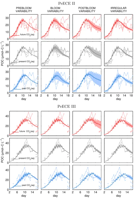
The model simulates the results from the Pelagic Enrichment CO₂Experiment (PeECE), a set of 9 outdoor mesocosms placed in coastal waters close to Bergen (Norway) dur- ing the spring 2003 (PeECE II) and the spring 2005 (PeECE III). In both experi- ments, blooms of the natural phytoplankton community were induced and treated in three replicates for future, present and past CO₂ conditions [Engel et al., 2008, Schulz et al., 2008, Riebesell et al., 2007, Riebesell et al., 2008]. Experimental data are avail-

9

DIN DH _N

DIC

r*

N-uptake

C-uptake s

r*

Phy

Phy

L*

DH _C

Figure 2.1. Representation of model equations. Dashed lines are fluxes that are only present in the model of POC dynamics (PeECE experiments) but not in the model of phytoplankton dynamics (BIOACID II indoor experiments). DIC, PAR and temperature are the environmental stressors.

able through the data portal Pangaea (doi: 10.1594/PANGAEA.723045 for PeECE II and doi: 10.1594/PANGAEA.726955 for PeECE III). Different species succeeded in the experiments, Emiliania huxleyi was the major contributor to POC in PeECE II [Engel et al., 2008] but also diatoms significantly bloomed during PeECE III [Schulz et al., 2008]. The same parameter set is applied for both experiments as is given in Table 2.1.

Field data of aquatic CO2 concentration, temperature and light, were taken as direct model inputs (Fig. A.2). Measurements of phytoplankton abundance, biomass or species composition were controversial. Instead, POC, PON and DIN serve for model calibra- tion. POC and PON data were adjusted for a direct comparison with model results (see SectionA.3), since some contributions to POC remain unresolved by our dynamical equations. In fact, state variables of our model comprise carbon and nitrogen content of phytoplankton, Phy_Cand Phy_Nand dissolved inorganic nitrogen, DIN, as representative for all nutrients. The dynamics of non phytoplanktonic components DH, i.e. detritus and heterotrophs, are distinguished by DH_C and DH_N, such as POC = Phy_C+ DH_C and PON = Phy_N+ DHN. Then, the dynamics of the state variables for PeECE model

2.1. Model of particulate organic carbon under acidification conditions 11

is given by

dPhy_C

dt = (P-R-L)·Phy_C (2.1)

dPhy_N

dt = V·Phy_C−L·Phy_N (2.2)

dDIN

dt = r·DH_N−V·Phy_C (2.3)

dDHC

dt = L·Phy_C−(s·DHC+ r)·DHC

(2.4)

dDH_N

dt = L·Phy_N−(s·DH_N+ r)·DH_N (2.5)

Initial conditions are estimated from experimental data as Phy_C(0) = 2.5µmol-C L⁻¹, Phy_N(0) = 0.4µmol-N L⁻¹and DIN= 8µmol-N L⁻¹for PeECE II and DIN= 14µmol-N L⁻¹ for PeECE III.

Primary production and respiratory terms are described in 2.3. Loss rate of phy- toplankton biomass is a density dependent term

L = L^∗·(Phy_C+ DH_C).

The resulting matter flux increases the biomass of detritus and heterotrophs (DH) and a fraction of it becomes part of the remineralizable pool. A temperature dependent remineralization term [Schartau et al., 2007]

r = r^∗·f_T

describes any kind of DIN production, as hydrolysis and remineralization of organic matter, excretion of ammonia directly by zooplankton and rapid remineralization of fecal pellets produced also by zooplankton. The other fraction of the non phytoplanktonic biomass is removed by settling with a rate related to the sinking coefficient, s, given in Eqs. 2.1 and 2.1. Our model is calibrated with experimental data from enclosed mesocosms where aquarium pumps ensured mixing. Therefore we assume that wealthy enough organisms were able to achieve neutral buoyancy [Boyd and Gradmann, 2002]

thus sinking does not directly affect phytoplankton biomass.

The CO2 effect on POC dynamics

This model reproduces the mean of PON, POC and DIN experimental data per treat- ment (Fig. 2.4). For PeECE II, PON is moderately overestimated and postbloom POC

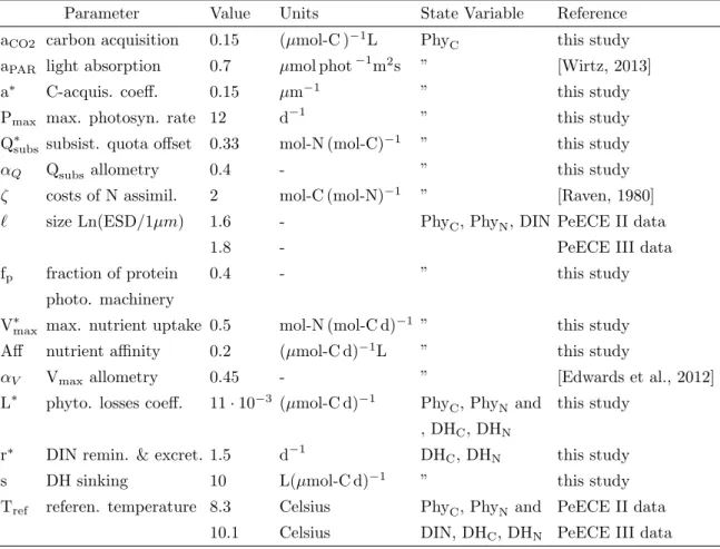
Table 2.1. Parameter values used for the reference run of PeECE experimental data. All values are common to both PeECE II and III experiments, only the mean temperature (determined by environmental forcing) and the averaged cell size in the community are different.

Parameter Value Units State Variable Reference

aCO2 carbon acquisition 0.15 (µmol-C )⁻¹L Phy_C this study a_PAR light absorption 0.7 µmol phot⁻¹m²s ” [Wirtz, 2013]

a^∗ C-acquis. coeff. 0.15 µm⁻¹ ” this study

Pmax max. photosyn. rate 12 d⁻¹ ” this study

Q^∗_subs subsist. quota offset 0.33 mol-N (mol-C)⁻¹ ” this study

α_Q Q_subsallometry 0.4 - ” this study

ζ costs of N assimil. 2 mol-C (mol-N)⁻¹ ” [Raven, 1980]

` size Ln(ESD/1µm) 1.6 - Phy_C, Phy_N, DIN PeECE II data

1.8 - PeECE III data

fp fraction of protein 0.4 - ” this study

photo. machinery

V^∗_max max. nutrient uptake 0.5 mol-N (mol-C d)⁻¹ ” this study

Aff nutrient affinity 0.2 (µmol-C d)⁻¹L ” this study

αV Vmax allometry 0.45 - ” [Edwards et al., 2012]

L^∗ phyto. losses coeff. 11·10⁻³ (µmol-C d)⁻¹ Phy_C, Phy_N and this study , DHC, DHN

r^∗ DIN remin. & excret. 1.5 d⁻¹ DHC, DHN this study

s DH sinking 10 L(µmol-C d)⁻¹ ” this study

T_ref referen. temperature 8.3 Celsius Phy_C, Phy_N and PeECE II data 10.1 Celsius DIN, DHC, DHN PeECE III data

2.2. Model of phytoplankton under acidification and warming conditions 13

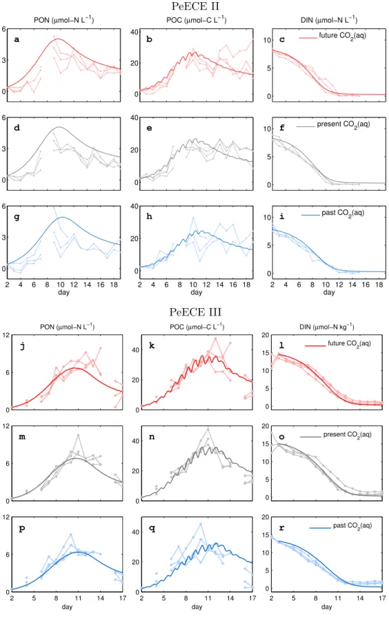
is slightly underestimated. Even so, the model fits the experimental data with similar precision than the treatment mean of the experimental data (see Table A.1). Treatment means and their associated standard deviations are typically used to describe experi- mental data (see Fig. 1b in [Engel et al., 2008] for PeECE II or Fig. 8a in [Schulz et al., 2008] for PeECE III) and are the foundations of statistical inference tools, which did not detect acidification responses for PeECE II and III. However, with our mechanistic model-based analysis, POC time series under future CO₂ conditions suggests an earlier and elevated bloom with respect to past CO2 conditions (Fig. 2.3).

2.2 Model of phytoplankton under acidification and warm- ing conditions

Data integration and dynamics of the state variables

A simplification of the previous model represents the reference dynamics of phytoplank- ton growth and decay by the temporal evolution of the state variables carbon and nitro- gen content of phytoplankton, Phy_C and Phy_N and dissolved inorganic nitrogen, DIN

dPhy_C

dt = (P-R-L)·Phy_C dPhy_N

dt = V·Phy_C−L·Phy_N (2.6)

dDIN

dt = −V·Phy_C.

This model is calibrated with phytoplankton abundance data (we lack this information for the model shown in the previous Section) from the indoor mesocosm experiments with plankton autumn communities of Kiel fjord (Germany) in 2012 (doi.10.1594/PANGAEA.840852 for BIOACID II), a factorial set-up at high and low CO₂ conditions and 9 and 15 Cel- sius temperatures. Phytoplankton bloom consisted mainly in diatoms. Environmental forcings showed in Fig. A.2 are implemented as model inputs. Initial conditions are es- timated from experimental data as Phy_C(0) = 1µmol-C L⁻¹, Phy_N(0) = 0.1µmol-N L⁻¹ and DIN= 10µmol-N L⁻¹.

Primary production and respiratory terms are described in Section 2.3. We as- sume grazing is the main cause of phytoplankton biomass removal as suggested by [Paul et al., 2015]. A relationship between an increase in their production and an increase in

PeECE II

0 3 6

PON (µmol−N L⁻¹)

a

0 20 40

POC (µmol−C L⁻¹)

b

0 5 10

DIN (µmol−N L⁻¹)

c ^{future CO2(aq)}

0 3 6

d

0 20 40

e

0 5

10 f ^{present CO2(aq)}

2 4 6 8 10 12 14 16 18 0

3 6

day

g

2 4 6 8 10 12 14 16 18 0

20 40

day

h

2 4 6 8 10 12 14 16 18 0

5 10

day

i ^{past CO2(aq)}

PeECE III

0 6 12

PON (µmol−N L⁻¹)

j

0 20 40

POC (µmol−C L⁻¹)

k

0 5 10 15 20

DIN (µmol−N kg⁻¹)

l ^{future CO}2(aq)

0 6 12

m

0 20 40 n

0 5 10 15 20

o ^{present CO}2(aq)

2 5 8 11 14 17

0 6 12

day

p

2 5 8 11 14 17

0 20 40

day

q

2 5 8 11 14 17

0 5 10 15 20

day

r ^{past CO}2(aq)

Figure 2.2. Reference runs for POC, PON and DIN simulating the mean of the replicates per treatment are in solid lines, with different colors for the three experimental CO2set-ups. Dots are three times replicated data from the Pelagic Enrichment CO2Experiment (PeECE II and III).

2.2. Model of phytoplankton under acidification and warming conditions 15

0 5 10 15 20

day 0

5 10 15 20 25 30 35 40

modeled POC (µmol-C L-1 )

PeECE II future CO

2(aq) past CO₂(aq)

0 5 10 15 20

day PeECE III

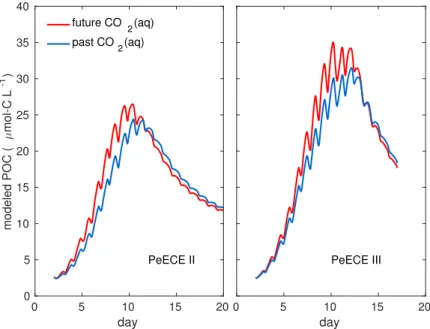
Figure 2.3. Reference simulations of POC for high CO2(red) and low CO2 (blue) experimental conditions show and earlier and more intense bloom under acidification conditions.

temperature has often been observed [Weisse and Montagnes, , Montagnes and Lessard, 1999, Rose, 2007], then phytoplankton biomass losses, L, are temperature dependent.

Therefore zooplankton effect is parametrized as L = L^∗·f^zoo_T with f^zoo_T described by the Arrhenius equation for protein folding as in Eq. 2.8. Parameters are given in Table 2.2

Warming and CO₂ effects on phytoplankton dynamics

Our model for BIOACID II data reproduces the mean of phytoplankton and nutrients dynamics. Reference runs are shown in Fig. 2.4. Phytoplankton carbon is moderately overestimated for the treatment with high temperatures and low acidification, while un- derestimated for the cold treatments. Even so, the model fits the experimental data with similar precision than the treatment mean of the experimental data (see Table A.1). With our mechanistic model-based analysis, phytoplankton growth in acidified environment shows an earlier and elevated bloom with respect to past CO2 conditions (see Fig. 2.5) as showed for POC in the previous model. About temperature, our model reproduces the effect reported in [Paul et al., 2015], i.e. a phytoplankton carbon Phy_C decreases by more than half with increasing temperature at bloom time. Synergistic effects of warming and acidification in phytoplankton biomass were not detected by sta-

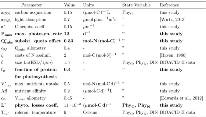
Table 2.2. Parameter values used for the reference run of BIOACID II indoor mesocosms data.

Due to linearity constrains specific to our method, only uncertainties in parameters in bold are explored with .

Parameter Value Units State Variable Reference

aCO2 carbon acquisition 0.15 (µmol-C )⁻¹L Phy_C this study a_PAR light absorption 0.7 µmol phot⁻¹m²s ” [Wirtz, 2013]

a^∗ C-acquis. coeff. 0.15 µm⁻¹ ” this study

Pmax max. photosyn. rate 12 d⁻¹ ” this study

Q^∗_subs subsist. quota offset 0.33 mol-N(mol-C)⁻¹ ” this study

αQ Q_subsallometry 0.4 - ” this study

ζ costs of N assimil. 2 mol-C (mol-N)⁻¹ ” [Raven, 1980]

` size Ln(ESD/1µm) 1.5 - Phy_C, Phy_N, DIN BIOACID II data

fp fraction of protein 0.4 - ” this study

for photosynthesis

V^∗_max max. nutrients uptake 0.5 mol-N (mol-C d)⁻¹ ” this study

Aff nutrient affinity 0.2 (µmol-C d)⁻¹L ” this study

αV Vmax allometry 0.45 - ” [Edwards et al., 2012]

L^∗ phyto. losses coeff. 11·10⁻³ (µmol-C d)⁻¹ Phy_C, Phy_N this study T_ref referen. temperature 9 Celsius Phy_C, Phy_N, DIN BIOACID II data

tistical inference tools described in [Paul et al., 2015]. With our mechanistic description for the reference dynamics per treatments we observe that acidification effects on bloom intensity are amplified at low temperatures, revealing acidification and warming may have antagonistic effects on plankton communities.

2.3 Definition of relative growth rate

Relative growth rateµis calculated from primary production rate subtracting respiration and mortality losses,µ= P−R−L. Mortality losses were already described in previous sections, thus we develop here the representation of P and R.

2.3. Definition of relative growth rate 17

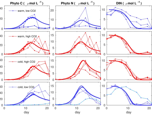
0 20 40

Phyto C ( µmol L ^-1)

warm, low CO2

0 20

40 warm, high CO2

0 20 40

60 cold, high CO2

0 10 20

day 0

20 40

60 cold, low CO2

0 10 20

Phyto N ( µmol L^-1)

0 5 10 15

0 5 10 15

0 10 20

day 0

5 10 15

0 5 10

DIN ( µmol L^-1)

0 5 10

0 5 10

0 10 20

day 0

5 10

Figure 2.4. Model reference runs for phytoplankton biomass reproducing the mean of the repli- cates per treatment are in solid lines, with different legend for the temperature (warm and cold) and CO2 (high and low) treatments. CO2 measurements were collected per mesocosm and those data are taken as model inputs (see Fig. A.2), which produce different model solutions per repli- cate (only visible for the treatment in the last raw). Dots are three times replicated data from BIOACID II indoor mesocosm experiments. Aberrant trajectory in the last row shows a malfunc- tioned replicate that we exclude of our analysis, following [Sommer et al., 2015].

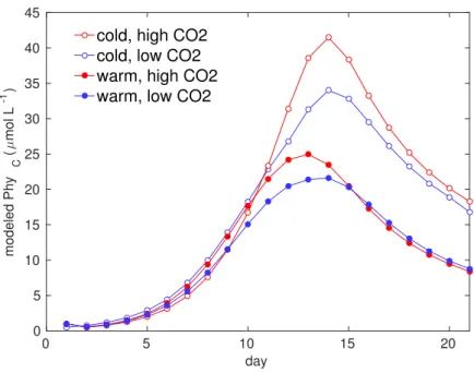
0 5 10 15 20 day

0 5 10 15 20 25 30 35 40 45

modeled Phy C (µmol L-1 )

cold, high CO2 cold, low CO2 warm, high CO2 warm, low CO2

Figure 2.5. Comparison of model reference runs for phytoplankton biomass reproducing the mean of the replicates per treatment. Model projections show that warming and acidification affects bloom intensity and timing.

Primary production

Primary production rate reflects the limiting effects of light, dissolved inorganic carbon (DIC), temperature and nutrient internal quota,

(2.7) P = Pmax·f_PAR·f_CO2·f_T·f_Q·fp.

P_maxis the maximum primary production rate. Specific light f_PAR depends on light and DIC. PAR for the indoor mesocosm experiment was provided by lamps. For outdoor experiments, we calculate the attenuation coefficient, a_z, considering that in coastal regions light intensity is reduced to 1% of its surface value typically in 5 m [Denman and Gargett, 1983] and that about 80% of the incident light passes through the mesocosm upper cover [Schulz et al., 2008]. We obtain a_z = 0.75m⁻¹. Then, spatially averaged PAR experienced by cells at mixed layer depth (MLD= 4.5m, [Engel et al., 2008]), is calculated from radiation at water surface, PAR₀ (shown in Fig. A.2), following an exponential decay described by the Lambert-Beer law

hPARi_z = PAR0

M L

Z M LD 0

e^−az·zdz.

2.3. Definition of relative growth rate 19

The relationship between photosynthesis and irradiance can be formulated referring to a cumulative one-hit Poisson distribution [Ley and Mauzerall, 1982,Dubinsky et al., 1986].

With the temperature and carbon acquisition dependence, it yields fPAR =

1−e

−a_PAR· hPARi_z P_max·f_CO2·f_T

,

where a_PAR is the effective absorption related to the chloroplast cross-section and sat- uration response time for receptors [Geider et al., 1998a, Wirtz and Pahlow, 2010], the carbon acquisition term f_CO2, Eq. 2.9. f_T is the temperature dependence. We consider that all metabolic rates depend on protein folding that increases with rising temperature following the Arrhenius equation [Scalley and Baker, 1997] as described in [Geider et al., 1998b] or [Schartau et al., 2007]

(2.8) f_T =e

−Ea·1 T− 1

T_ref

,

with activation energy E_a = ^T₁₀^2ref ·log(Q₁₀) as in [Wirtz, 2013], and T_ref is the mean measured temperature (see Fig. A.2). For PeECE experiments we take Q₁₀ = 1.88 for phytoplankton [Eppley, 1972, Brush et al., 2002]. In the indoor experiments, we use Q₁₀ = 1.48 for diatoms [Suzuki and Takahashi, 1995]. For zooplankton, a higher value, Q10= 2.5, represents enhanced metabolism under warming conditions.

According to [Peters, 1983, Brown et al., 1995, Bonner, 2006], among others, size is a driving force for all of biology because it determines important biological features as strength, surface area, complexity, rate of metabolism, organism abundance, turn over or life span. About phytoplankton, several studies unearthed the importance of size to describe metabolic rates [Peters, 1983,Marb`a et al., 2007]. In particular, recent empirical and theoretical studies described the relation of phytoplankton size with subsistence quota, light acquisition or nutrient and carbon uptake by allometric relations [Litchman and Klausmeier, 2008,Litchman et al., 2009,Wirtz, 2011], as well as how size-dependences scale from cellular to ecosystem level [Litchman et al., 2007, Litchman et al., 2010].

Taking this into account, the mean cell size in the community is a suitable way to include species composition and size structure in marine ecosystem models, which is relevant since we aim to investigate how much uncertainties in community composition among replicates may escalate into high variability within a treatment. Here the mean cell size in the community is represented as the logarithm of the mean equivalent spherical diameter ESD, `=Ln(ESD/1µm).

To resolve sensitivities to different DIC conditions, we seek for a relatively accurate description of carbon acquisition as a function of DIC and size. It has been suggested by previous observations and models that ambient DIC concentration increases primary production [Schluter et al., 2014, Rost et al., 2003, Zondervan et al., 2001, Riebesell et al., 2000, Chen, 1994, Riebesell et al., 1993] and mean cell size in the community [Sommer et al., 2015, Eggers et al., 2014, Tortell et al., 2008]. We adopted and simplified a biophysically explicit description for carbon uptake from [Wirtz, 2011], where the efficiency of intracellular DIC transport has been derived as a function of mean cell size and CO₂ concentration. For very large cells, the formulation converges to the surface to volume ratio, that in our notation readse<sup>−`</sup>. By contrast, the allometric dependence of primary production on CO<sub>2</sub> does not apply to picophytoplankton so that together we have a non-uniform allometric scaling fCO2(`) in the carboxylation rate

(2.9) f_CO2 = 1−e^−aCO2·CO2

1 + a^∗·e^{(`−aCO2·CO2)}

.

The specific carbon absorption coefficient a_CO2 reflects size-independent features of the DIC acquisition machinery, such as carbon concentration mechanisms [Raven and Beardall, 2003].

The allometric factor α_Q quantifies the scaling relation of subsistence quota and cell size. We use a Droop dependency on nutrient N:C ratio [Droop, 1973] which has been recently mechanistically derived [Wirtz and Pahlow, 2010, Pahlow and Oschlies, 2013]

f_Q=

1−Q_subs Q

where Q = Phy_N

Phy_C. Its lower reference, the subsistence quota Q_subs = Q^∗_subs·e^−αQ·`, is considered size dependent to reflect a lower protein demand for uptake mechanisms in large cells [Litchman et al., 2007].

The last term in Eq. 2.7 accounts for an energy allocation trade-off in phytoplank- ton cells: protein allocation for photosynthetic compounds as RuBisCo and pigments, fp, versus allocation for nutrient uptake, fv, expressed by fp+ fv = 1. Since we are concerned about variability reconstruction rather than in the most accurate description, for instance, based on optimal allocation [Wirtz and Pahlow, 2010, Pahlow and Oschlies, 2013], we favored a simplify detailed partition models by setting the trait fractions con- stant. In stead of describing trait variations, we describe trade-offs in steady state in

2.3. Definition of relative growth rate 21

terms of size and energy allocation, for constraining the parametrization during the cal- ibration process. The explicit account for trade-off steps towards a more mechanistic description of the growth rate.

Respiratory cost and nutrient uptake rates

Efforts related to nutrient uptake V are represented by a respiration term because basic maintenance respiration expenses are neglected [Wirtz and Pahlow, 2010]. Respiration rate is then calculated as

R =ζ·V

where ζ expresses the specific respiratory cost of nitrogen assimilation [Raven, 1980, Aksnes and Egge, 1991, Geider et al., 1998b, Pahlow, 2005]. For simplicity, our model merges the set of potentially limiting nutrients (e.g. P, Si and N) to a single resource only, that is DIN. We follow [Aksnes and Egge, 1991] as described in [Pahlow, 2005] for the maximum uptake rate

Vmax= 1

1 V^∗_max·fT

+ 1

Aff·DIN ,

comprising the maximum uptake coefficient, V^∗_max, and the nutrient affinity, Aff. Besides adding a temperature dependence of nutrient uptake as given in [Schartau et al., 2007], we assume that respiratory costs decrease with increasing cell size [Edwards et al., 2012]

which leads to an allometric scaling in nutrient uptake [Wirtz, 2013] with exponent αV. We also account for the static proteins allocation trade-off between photosynthetic machinery, fp, and nutrients uptake, fv= 1−fp. Then the nutrient uptake term is

V = (1−fp)·Vmax·e^−αV·`.

3

Propagation of static uncertainties

3.1 Method

In this chapter we perform an uncertainty propagation analysis with the reference dy- namics described in Section 2.1. Variability induced by uncertainties simulated as varia- tions of the model control factors is compared with the variability in POC experimental data. The comparison between simulated and experimental variability in POC helps us to identify those changes in physiological state and in community structure that are main potential contributors to the variability.

We consider 19 model factors, φ_i, with i= 1, ..., N = 19, made of 14 process pa- rameters and 5 initial conditions for the state variables in Eqs. 2.1. In Table 2.1 we show the reference values,hφ_ii, where brackets denote ensemble average. Factor variations are introduced as random values within the variational range [hφ_ii − 4φ_i,hφ_ii+4φ_i], where 4φ_i is the standard deviation of the normal distribution of possible factor values. To calculate 4φ_i, we first generate 10⁴ simulations, each one with a different factor value, φi. The ensemble of model solutions represents possible replicate realizations (see Fig.

3.1). The factor value for each POC trajectory is randomly drawn from a normal distri- bution around the factor reference valuehφ_ii, which is the residual distribution assumed by parametric statistical inference tools as ANOVA [Field et al., 2008]. We take the en- semble average over modeled replicates and calculate the standard deviation,4POC^mod_i . Then4φ_iis the standard deviation of the distribution of factor values such as4POC^mod_i does not exceed the standard deviation of the experimental POC data, 4POC^exp, at

23

any mesocosm, at any time. This comprises a Monte Carlo non intrusive sampling base method for uncertainty quantification [Chantrasmi and Iaccarino, 2012]. The effect size of variations ofφi on the variability is then

(3.1) εi= (4POC)^mod_i

4φ_i .

This effect size expresses the maximum variability a factor can generate, 4POC^mod_i , relative to the range of factor variations, 4φ_i, to ensure 4POC^mod_i is the closest to 4POC^exp at any time. More generally,ε_i relates the uncertainty of a variable X (here X=POC) and the uncertainty of the input factors φ_i on which it depends (that in our application quantifies how much variability in experimental observables derives from cell physiology and community structure)

(4X)² =

N

X

i=1

c²_i ·(4φ_i)² where ci = ∂X

∂φi are called sensitivity coefficients [Ellison and Williams, 2012]. This ex- pression is based on the assumption that changes inX in response to variations in one factor φ_i are independent from those due to changes in another factor φ_j and that all changes are small, thus cross terms and higher order derivatives are negligible. Where no reliable mathematical description of X(φ_i) exists, c_i can be evaluated directly by experiment [Ellison and Williams, 2012]. As in our case only the rate equation for POC changes is known, but not its analytical solution, and, as mentioned in the Intro- duction, such measurements are costly in mesocosm experiments, we obtain equivalent information through the numerical calculation of the corresponding effect sizes εi. In the following, the standard deviation of the factors, i.e. factors uncertainty4φ_i will be given as percentage of the reference values and will be called 4Φ_i. The actual factor range is given by: 4φ_i = 4Φ_i·φi

100 . Strong heteroscedasticity, i.e. irregularities in the standard deviations of experimental POC data (see, for instance, small 4POC^exp at day 8 in Fig. 2.2p), translates into drastically enhanced effect sizes if the model-data comparison would be done at a daily basis. For this reason we consider the temporal mean of the standard deviation per phase, i.e. prebloom, bloom, and postbloom. We inferred phases for PeECE II from [Engel et al., 2008] and for PeECE III from [Schulz et al., 2008] and [Tanaka et al., 2008]). For the first experiment, phytoplankton main bloom is estimated to occur from day 7 to day 13 and for the second experiment, from day 7 to day 11.

3.2. Results 25

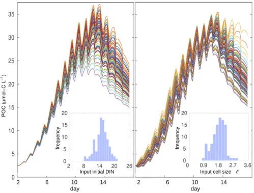
2 6 10 14

day 2 6 10 14 day

Input initial DIN

frequency frequency

Input cell size

Figure 3.1. Examples of 10² model projections of POC for the past CO2 treatment in PeECE III. In the left panel, model outputs with slight variations in initial nutrient concentration and in the right panel, with slight input variations in mean cell size. Histograms show input distribution with meanhφiiand standard deviation4φigiven in Tables 2.1 and 3.1, respectively. To calculate system tolerances and uncertainties effect sizes, we numerically calculate 10⁴ model realizations, thus the distribution of input factors is closer to normal.

To numerically calculate the ensemble of 10⁴ POC trajectories that simulate ex- perimental replicate outcomes (Fig. 3.1), we apply the Heun integration method (see Section B.1. A second order numerical method is required to obtain conservative tra- jectories at the chosen step length, h = 4·10⁻⁴ (approx. 35 seconds of experimental time) despite the presence of oscillations (see PAR forcing, Fig. A.2). The number of modeled POC time series is chosen ensuring convergence, such as a higher number of model realizations, i.e. a higher number of modeled replicates, will produce the same results.

3.2 Results

Our method allows for a factor specific variability decomposition (4POC)^mod_i of the total variability in Fig. 3.2. While intensity decomposition is provided by the calcu-

lation of the effect size, also temporal decomposition is available, by grouping factors variations depending on the timing of their effect (Fig. 3.3). To identify the nature of the uncertainties (i.e. to which factor they belong to), their corresponding inten- sity (i.e. the effect size) and the timing of their escalation (i.e. when the variability amplification occurs) provide valuable information for experimental design and interpre- tation of empirical data. For example, when an experiment is designed to identify a potential effect during the bloom, uncertainties in factors triggering variability during the bloom are more relevant than the ones triggering variability during the potbloom (thus the latter need not to be subject to intensive monitoring), and among the factor uncertainties triggering variability during the bloom, we can identify which contribute the most, and consequently, we can concentrate experimental efforts in the control of these factors, when possible. If it is known that an experiment lacked accuracy in one of these factors, uncertainty propagation is then a suitable explanation for controversial conclusions extracted from statistical inference analysis, for instance, in cases when sim- ilar experiments detect an acidification effect while others fail to detect an effect (Type II error [Field et al., 2008]).

Variability during the prebloom phase can be explained mainly by variations of factors related to subsistence quota, i.e. Q^∗_subs and αQ in both PeECE II and III ex- periments (left column in Fig. 3.3). This means that variations in subsistence quota first intensify the divergence of POC trajectories, to be damped few days later by the system dynamics. These subsistence parameters only need to vary about 6% and 8%

among replicates (see Table 3.1), to maximize their contribution to the4POC^exp, thus their effect size is the highest (see Fig. 3.4). Variations in initial nutrient concentration, DIN(0), mean cell size, `, and phytoplankton biomass loss coefficient, L^∗, generate the modeled variability mainly during the bloom (with just about 20% differences among replicates, see Table 3.1 and second column in Fig. 3.3) showing high values of effect size (gray highlight in Fig. 3.4). Amplified variability in the postbloom phase (third column in Fig. 3.3) emerges from uncertainties in the reference temperature T_ref for the Arrhenius equation, Eq. 2.8, in sinking loss or export flux, s, and in remineralization and excretion,r^∗. Effect size of Tref is high, with just about 12% variation. To generate the high divergence during the postbloom, a strong perturbation of parameters relevant for the non phytoplanktonic biomass is needed (about 81% of the reference value for sinking and 96% for remineralization and excretion, see Table 3.1), which translates to

3.3. Discussion 27

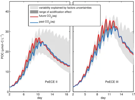
2 6 10 14 18

0 10 20 30 40

POC (µmol−C L−1)

day PeECE II

2 5 8 11 14 17

PeECE III

day variability explained by factors uncertainties range of acidification effect

future CO 2(aq) past CO₂(aq)

Figure 3.2. Reference simulation of POC for high CO2 (red) and low CO2 (blue) experimental conditions bound the range of acidification effect (dark gray) according to our model projections.

Light gray is limited by the modeled POC variability, (4POC)^mod, quantified as the standard deviation of numerically simulated replicates calculated with differences in model factors simulating experimental uncertainties.

a relatively low effect size. Variability throughout all bloom phases (right column in Fig. 3.3) follows from varying carbon and nitrogen initial conditions, Phy_C and Phy_N, nutrient uptake related factors, V^∗_max,α_V and Aff, and protein allocation for photosyn- thetical machinery, f_p. About the latter, high standard deviations of the tolerance (see Table 3.1) suggests non conclusive results.

Interestingly, effect sizeεi is low for carbon acquisition aCO2 and light absorption a_PAR. Perturbations of the initial detritus concentration, DH_C(0) and DH_N(0) also have no impact on the dynamics as long as they were within reasonable ranges (4Φ_i <100).

In fact, more than tenfold differences among replicates in such non relevant factors were necessary to achieve a perceptible (4POC)^mod_i .

3.3 Discussion

In this study we adapted a sensitivity analysis to assess factor variations that can affect experimental data, a perspective beyond the classical description of the mean system