A new mesocosm system to study the effects of environmental variability on marine species and communities

(1)

Limnology and Oceanography.

doi: 10.1002/lom3.10306

A new mesocosm system to study the effects of environmental variability on marine species and communities

Christian Pansch ,* Claas Hiebenthal

Department of Marine Ecology, GEOMAR Helmholtz Centre for Ocean Research Kiel, Kiel, Germany

Abstract

Climate change will shift mean environmental conditions and also increase the frequency and intensity of extreme events, exerting additional stress on ecosystems. Whilefield observations on extremes are emerging, experimental evidence of their biological consequences is rare. Here, we introduce a mesocosm system that was developed to study the effects of environmental variability of multiple drivers (temperature, salinity, pH, light) on single species and communities at various temporal scales (diurnal - seasonal): theKiel Indoor Benthocosms (KIBs). Both, real-time offsets fromfield measurements or various dynamic regimes of environmental scenarios, can be implemented, including sinusoidal curve functions at any chosen amplitude or frequency, stochastic regimes matching in situ dynamics of previous years and modeled extreme events. With temperature as the driver in focus, we highlight the strengths and discuss limitations of the system. In addition, we examined the effects of different sinusoidal temperature fluctuation frequencies on mytilid mussel performance. High- frequency fluctuations around a warming mean (+2C warming, 2C fluctuations, wavelength = 1.5 d) increased mussel growth as did a constant warming of 2C. Fluctuations at a lower frequency (+2 and2C, wavelength = 4.5 d), however, reduced the mussels’growth. This shows that environmentalfluctuations, and importantly their associated characteristics (such as frequency), can mediate the strength of global change impacts on a key marine species. The here presented mesocosm system can help to overcome a major shortcoming of marine experimental ecology and will provide more robust data for the prediction of shifts in ecosystem structure and services in a changing andfluctuating world.

Global climate models project warming and acidification of the world’s oceans (Rhein et al. 2013). At more regional scales, freshening of seawater (up to 5 units in the Baltic Sea), and increased eutrophication (as a consequence of intensifying agri- culture and increased riverine runoff) are expected (HELCOM 2007; The BACC Author Team 2008; Rabalais et al. 2009; Rhein et al. 2013). Furthermore, the interaction of eutrophication and warming (faster re-mineralization, lower gas solubility, and increased stable stratification) favors hypoxic conditions (Diaz and Rosenberg 2008; Rabalais et al. 2009; Gräwe et al. 2013). This ultimately leads to an additional increase of coastal acidification (Melzner et al. 2013; Waldbusser and Salisbury 2014). Superim- posed on these long-term trends, an increase in the variability around mean changes, particularly in the frequency, intensity,

and duration of climate extremes, is expected (Easterling et al.

2000; Meehl and Tebaldi 2004; Rahmstorf and Coumou 2011;

Rummukainen 2012; Christensen et al. 2013; Rhein et al. 2013).

Both, shifts in the meansandin the variability of environmental factors, will most likely change key biological processes and alter the structure and functions of pelagic and benthic marine ecosystems (Pörtner et al. 2014; Pansch et al. 2018).

Effects of changedglobal meansof single factors, like warming, acidiﬁcation, desalination, eutrophication or hypoxia, on single species have been investigated in numerous manipula- tive experiments andﬁeld observations (Pörtner et al. 2014).

Experimental investigations testing multiple stressor impacts on single species (Harvey et al. 2013; Kroeker et al. 2013), as well as on communities (Graiff et al. 2015; Queiros et al. 2015;

Falkenberg et al. 2016) revealed synergistic, additive, and antagonistic effects of different stressors (Gunderson et al.

2016). Yet, while temperature shifts have been shown to be the most prevalent and effective driver of changes in marine systems (Pörtner 2008; Harvey et al. 2013; Koch et al. 2013;

Kroeker et al. 2013; Graiff et al. 2015), recent reviews empha- size the limits of our current knowledge with respect to shifts predicted under climate change (Andersson et al. 2015;

*Correspondence: ch.pansch@gmail.com

Additional Supporting Information may be found in the online version of this article.

This is an open access article under the terms of the Creative Commons Attribution License, which permits use, distribution and reproduction in any medium, provided the original work is properly cited.

(2)

Riebesell and Gattuso 2015). An up-scaling from single species to the community and ecosystem level, from single to multiple driver experiments, and from short-term incubations to long-term adapted species and communities is therefore considered the logical next step (Andersson et al. 2015; Riebesell and Gattuso 2015). However, a severe shortcoming of most marine studies at all levels of complexity, is the exclusion of ﬂuctuations of abiotic (and biotic) drivers from the experimental designs (Thompson et al. 2013; Boyd et al. 2016; Gunder- son et al. 2016; Wahl et al. 2016; Morash et al. 2018).

Marine biological systemsﬂuctuate at various temporal and spatial scales (Hofmann et al. 2011; Frieder et al. 2012; Wahl et al. 2016). Climate dynamics (e.g., anthropogenic shifts, North Atlantic Oscillation, El Niño/La Niña events (Soares et al. 2014)), seasons (Frankignoulle and Bouquegneau 1990;

Thomsen et al. 2010), weather and discrete upwelling or down-welling events (Feely et al. 2008; Saderne et al. 2013), tides, as well as biological activities (e.g., respiration and photosynthesis; Hofmann et al. 2011; Buapet et al. 2013; Saderne et al. 2013) impose shifts at temporal scales of decades, years, months, weeks and days to hours or seconds, respectively (partly reviewed in Boyd et al. 2016). In particular, shallow habitats feature stronglyﬂuctuating environmental conditions (Duarte et al. 2013; Waldbusser and Salisbury 2014) with the potential of exerting intense transient stress at the organismic and community level.

Climate variability is expected to increase along with a gen- eral climate change (Meehl and Tebaldi 2004; Rahmstorf and Coumou 2011; Gräwe et al. 2013). As a consequence, terrestrial ecologists have started to acknowledge the effects of environmental variability on species’performances and distributions, as well as their potential manifestation in community diversity, ecosystem functions, and services (Ruel and Ayres 1999; Bozino- vic et al. 2011; Estay et al. 2011; Paaijmans et al. 2013). Recent modeling indicates that increased temperature variation causes a greater harm to terrestrial ectothermic invertebrates than mean climate warming (Vasseur et al. 2014). For marine systems data are rare. Field observations show that extreme climatic events can permanently alter marine ecosystems (Reusch et al.

2005; Garrabou et al. 2009; Wernberg et al. 2013). Experimental approaches are of particular value because they provide ade- quate controls and facilitate causation-based inferences by precise manipulation of conditions such as forecasted extremes that have not yet occurred (Sommer 2012). Experiments allow for replicated and repeatable tests of hypotheses and for the evaluation of responses of interacting organisms and factors, with the potential to feed data into large-scale models (Nouguier et al. 2007; Petersen et al. 2009). Initial experimental data show that an applied variability around means of drivers such as pH (Cornwall et al. 2013; Frieder et al.

2014; Eriander et al. 2015), oxygen (Neilan and Rose 2014), or temperature (Winters et al. 2011) can differently impact marine species when compared to mean constant shifts of the driver in focus. Biogenic ﬂuctuations of the carbonate

system, for example, have recently been shown to mitigate the effects of acidiﬁcation on benthic calciﬁers (Cornwall et al. 2014; Wahl et al. 2018).

From a theoretical perspective, and taken that a biological response to any environmental driver is curvilinear (e.g., bell- shaped with an intermediate optimum), according toJensen’s inequality, any variation around a sub- or supra-optimal mean value should lower the performance of an organism (Ruel and Ayres 1999). In addition, environmental fluctuations as well as extremes of environmental drivers can generally lead to species’ range shifts and/or lethally impact genotypes and species—with the potential to raise the ratio of more plastic or robust genotypes/species in the surviving populations or communities (Reusch et al. 2005; Wernberg et al. 2013; Manenti et al. 2014; Karve et al. 2016; Pansch et al. 2018). Indeed, strong evidence was found that populations prone to large fluctuations in stressful conditions (e.g., by acidification, eutrophication and/or organic pollutants) are more robust than comparable populations living in habitats characterized by less environmental variability (Pansch et al. 2014; Huhn et al. 2016; Thomsen et al. 2017). Environmentalfluctuations typically alternate between extreme stress conditions (that eliminate sensitive genotypes or species) and phases of temporal relaxation from stress (which represent a transient refuge from stress and may allow survivors to recover (Wahl et al.

2016)). This aspect of stress release and the ecological consequences resulting from it, however, are so far almost entirely neglected in experimental climate change research (Manzello 2010; Gunderson et al. 2016; Wahl et al. 2016, 2018).

Transient deviations from stressful conditions have an enormous potential to amplify (by means of adding additional stress to the system) or buffer (by enabling recovery) environ- mentally caused stress. Hence, results obtained from studies that apply constant stress regimes are of limited relevance to the real world. We therefore developed a mesocosm concept speciﬁcally designed to elucidate the role of natural environmental variability as an ampliﬁer or buffer of ecosystem changes. The innovative nature of this mesocosm facility allows for the application of dynamic regimes of multiple environmental drivers (temperature, salinity, and pH) including sinusoidal curves at any chosen amplitude or frequency ranging from minutes to months, stochastic regimes, in situ repetition of (logged) dynamics of previous years, and projected future extreme events. This line of research will most likely change the outcome of current predictions for future ecosystem changes.

As the focal driver of this study, we chose temperature because (1) the predicted temperature shifts are substantial and reliable (Rhein et al. 2013), (2) even slight temperature shifts have been shown to have comparably large biological effects (Pörtner 2008; Harvey et al. 2013; Koch et al. 2013;

Kroeker et al. 2013), and (3) temperature as a driver is independent of biological activity (unlike acidiﬁcation or eutrophication for instance (Wahl et al. 2018)), and (4) easy to control

(3)

experimentally. Other variables such as salinity as well as pH, however, were also manipulated inﬂuctuating modes and are discussed in this study.

Materials and procedures

Study system

The Baltic Sea represents an ideal model system to study the consequences of a changing climate. A strong scientific foundation, access to long-term data series as well as expected future changes of multiple climate drivers provide a unique opportunity to evaluate basic scientific questions and assess management actions and efficiency (Reusch et al. 2018). The Baltic Sea is an exceptionally young ecosystem (< 12k yr) characterized by a high coast to volume ratio, a hydrological sur- plus (precipitation and river inflow exceeds evaporation), a strong permanent (deep), and seasonal (shallow) stratification and a generally low metazoan biodiversity (HELCOM 2007;

The BACC Author Team 2008). The most characteristic features of the Baltic Sea are the pronounced West to North/East salinity gradient, which is the ultimate cause for a conspicu- ous biodiversity gradient from West (high) to East (low; Bleich et al. 2011; Zettler et al. 2014), and the occurrence of strong ﬂuctuations of many environmental variables such as temperature, salinity, oxygen, pH, and nutrients (Melzner et al. 2013;

Saderne et al. 2013; Pansch et al. 2014; Havenhand et al.

2018; Thomsen et al. 2013). In shallow regions of the Baltic Sea, temperatureﬂuctuations are prevalent at various temporal and spatial scales (Supporting Information Fig. S1) and, both, mean and variability of temperatures, are predicted to increase in the coming decades (Meehl and Tebaldi 2004; HELCOM 2007; The BACC Author Team 2008; Rahmstorf and Coumou 2011; Rhein et al. 2013).

In recent years, an increase in the frequency of summer heatwaves has been observed in the Baltic Sea region (Lehmann et al. 2011). Such seasonal temperatureﬂuctuations are further reinforced (or buffered) on a local scale by sporadic upwelling events importing cold, acidic, and hypoxic water into Baltic coastal shallow habitats (Melzner et al. 2013;

Saderne et al. 2013). In addition, in dense macrophyte belts, biogenic diurnal pHﬂuctuations of up to 1 pH unit (10-fold changes in H⁺concentration) are accompanied by substantial shifts in aragonite and calcite saturation states (Saderne et al.

2013; Wahl et al. 2016, 2018). With the availability of long- term datasets, a rich knowledge of currentfluctuations in environmental drivers and of robust estimations of future means, realistic amplitudes and frequencies of driver fluctuations as well as of simulated stochasticfluctuations and extreme events can be determined for future experiments.

Design of the infrastructure

We designed and constructed 12 indoor mesocosms to simulate natural environmental variability for experiments on marine benthic communities: theKiel Indoor Benthocosms(KIBs).

The infrastructure is located in a 60 m² constant temperature room (currently at 16C, but temperatures between 5C and 25C are possible) at the GEOMAR Helmholtz Centre for Ocean Research Kiel, Germany (5419⁰47.65⁰⁰N, 108⁰54.17⁰⁰E). An over- view of the facility and the main components of single mesocosm units are given in Fig. 1 (see also Supporting Information Fig. S2 for more details). The KIBs’basic concept was inspired by theKiel Outdoor Benthocosms(Wahl et al. 2015). However, they provide an additional asset of programmable multifactorial regimes and include dynamic irradiation regimes using advanced LED technologies, which produce an adjustable near- natural light spectrum.

The 12 mesocosms are made of PE (Polyethylene) tanks (Georg Utz Group System Container “Paloxe” 3-622) with a volume of 600 L each. Individual tank sizes are 920 × 1120 mm (inside measures) with a maximum water depth of 600 mm. The mesocosm system can be operated in closed- or open-circuit mode with a constant flow-through of natural, sand-filtered (GEOMAR central facility) seawater from Kiel Fjord. Flow rates can be high (up to 50 L per hour) with stable flows via gravity-fed standardized pipes from 60 L header tanks, (see Jokiel et al. 2014) or can be adjusted from 1 L to 50 L per hour by small aquarium taps (Rebie, Bielefeld, Ger- many). In addition, peristaltic pumps provide either a precise flow-through of seawater to the experimental tanks or constant/recurrent additions of food. During longer-term experiments (> 4 weeks) fouling (recruitment of target species or other organisms) on the surface of the inner walls of the mesocosms can either be evaluated and permitted, cleaned manually, or controlled to some degree byfilters or by grazers within a community (seeWahl et al. 2015).

Each of the 12 mesocosm units is equipped with a commercially available aquarium controller (Proﬁlux 3.1TeX; GHL Advanced Technology GmbH KG, Kaiserslautern, Germany).

Two power bars (Powerbar-5.1-D-PAB, GHL, Germany) represent a total of 10 controllable power sockets per mesocosm (Supporting Information Fig. S3). Controllers are connected serially via Profilux Aquatic Bus (PAB) enabling communication between single controller units and the different power bars. A LAN network connection enables external communication. The aquarium controllers allow for manipulation of temperature, salinity, pH (and optionally oxygen) and, at the same time, offer the possibility to log these parameters in the mesocosms continuously (sensors from GHL, Germany; Supporting Infor- mation Fig. S3). All data are saved as text (.csv)files and stored on a central computer for data visualization and storage. In addition, the aquarium controllers possess an alarm notification system via e-mail in case the set threshold values are exceeded.

For quality assurance and external validation, in addition to the data provided by the aquarium controllers, discrete light, temperature, salinity, pH, and oxygen measurements are carried out with HOBO temperature loggers (HOBO Pendant Light/

Temperature 16K Data Logger, Onset Computer Corporation), CTD salinity loggers (Star-Oddi, Reykjavik, Iceland), as well as

(4)

with a portable reference system (hand-held probe MULTI 3630 IDS, with sensors: SenTix 940, FDO 925, TetraCon 925;

Wissenschaftlich Technische Werkstätten, Weilheim, Germany).

Regular discrete water samples for total alkalinity (TA), nutrients, and dissolved inorganic carbon (DIC) are taken during experimental investigations (depending on the research question).

DIC and TA measurements are calibrated using certiﬁed seawater standards (Dickson, Scripps Institution of Oceanography, San Diego; Dickson et al. 2003, 2007).

All 12 fully independently controlled mesocosms can either be operated in a“regression mode” with up to 12 different

climate change scenarios (no replication), or in a factorial

“ANOVA mode” with present and future climate scenario treatments (3–6 replicates). Additionally, each of the 12 mesocosm units can serve as water bath for several experimental (sub-)units (EUs), e.g., 1 L or 2 L bottles, 4.5 L cell culture bottles or 18 L 600 mm deep PMMA (Plexiglas, acrylic glass) cyl- inders (Supporting Information Fig. S4). Target organisms or simplified communities can, thus, be either placed directly inside the 600 L mesocosms at operational water depths of up to 600 mm, or in an almost infinite (depending on size) num- ber of independent EUs. Treatment levels can be randomly Fig. 1.Kiel Indoor Benthocosms (KIBs) are established to simulate environmental parameters atfluctuating modes over extended periods using automated procedures. The 12 600 L mesocosms (A) are equipped with up-to-date controlling units, heaters, coolers, pumps and solenoid valves (not depicted) to control water temperature, salinity, and pH. Each unit (B,C) contains a pump (1) supplying water to a chiller (2), a pump (3) responsible for water mixing inside the mesocosm, thus enabling an equal distribution of heat, and another pump (4), which supplies water to the heat exchanger (5) in the 60 L header tank (6). The chiller and three heating units (7) regulate water temperatures measured by the aquarium controller sensors (GHL, Ger- many; 8) and aquarium controllers (not depicted). After passing through an in-house sandfilter, fresh seawater (B; light gray) runs into the header tank (#) and the mesocosm, or (as depicted here) the respective experimental units (EUs). From here, the wastewater (dark gray)flows into the mesocosm (to the chiller or the heat exchanger) and out of the system. Technical drawings were done by Dar Golomb (Lab Manager at The Rilov Lab“Marine Com- munity Ecology”at the National Institute of Oceanography, Haifa, 31080, Israel).

(5)

distributed across all 12 mesocosms, reducing the risk of block effects. Block (tank position) effects can also be tested for statistically: in case of no statistically signiﬁcant“block”effects, the data can be pooled between tanks; in the case of signiﬁ- cant effects, “block” can be included in the main statistical model as a random factor.

Additional features of the system such as the LED lights, the automated temperature control, the system for salinity and pH variability simulations and the manipulated feeding are described in more detail in the following paragraphs.

The KIB infrastructure is likely the most advanced infrastructure to date with regards to the ability to realistically simulate past, present, and future marine environmental ﬂuctuation scenarios of different drivers in a ﬂow-through system.

LED light system

Each mesocosm is equipped with LED light bars of two light colors (LEDaquaristik UG. Schierbusch, Germany), which are controlled via the aquarium controllers. Each mesocosm has eight 800 mm light bars (each with 54 LEDs, 25 W; www.

ledaquaristik.de; Supporting Information Fig. S2C). Four bars operate at “sunset” (eco+ LED bar SUNSET 3500K, 2356 Lumen) and four bars at“daylight”(eco+ LED bar DAY 5500K, 2575 Lumen) illumination wavelengths. Light wavelengths

and intensities can be programmed at constant and/orﬂuctuat- ing modes (including re-occurring cloud cover).

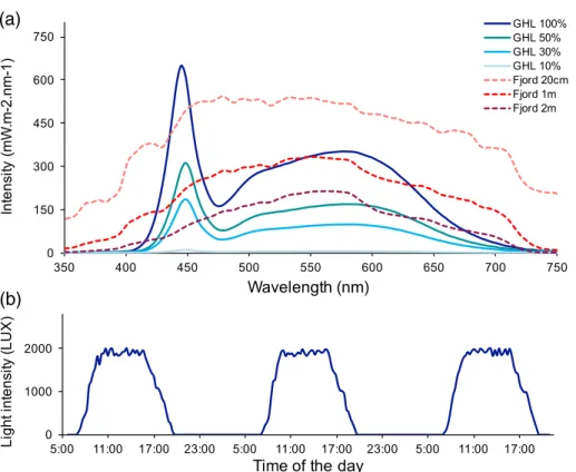
Natural light intensity was assessed in Kiel Fjord (GEOMAR Pier; 5419⁰48.69⁰⁰N, 10 8⁰59.68⁰⁰E), at depths of 0.2 m, 1 m, and 2 m, at noon, on 11^th July 2016 (cloud-free day), using a UV–VIS radiance sensor (Ramses-ACC-VIS, 320–950 nm, TriOS Science, Germany). Light intensity in the mesocosms was measured under one set of two sunset and two daylight light bars in December 2016. This way, we were able to accurately mimic natural Kiel Fjord summer sunny day light intensities (Fig. 2A).

LED light sources typically show a peak in the fraction of blue light within the visible spectrum (around 445 nm) and a wider secondary peak between 500 nm and 650 nm. Blue lightﬁlters may be applied if required. In addition, to represent light ramping abilities, day/night light regimes were recorded just above the surface of the 600 L mesocosms in April 2017, using a HOBO light and temperature logger. Data were recorded every second and means were calculated for 15-min intervals (Fig. 2B).

Automated temperature control system

Temperature manipulations can be run in three different modes: A (1)ﬁxed driver value mode, allows for long-term experimental investigations at any constant temperature between 4C and 35C. A (2) dynamic nominal value mode (Wahl et al. 2015) can represent a real-time offset fromﬁeld measurements for a reference system (e.g., the natural Kiel Fjord habitat). This allows for

(a)

(b)

Fig. 2.Light system for simulations of dynamic irradiation regimes with a near-natural spectrum using LED technologies. Light intensities were assessed in Kiel Fjord (at water depth 0.2 m, 1 m, and 2 m, dashed lines) and in a mesocosm at different levels of intensity (set by aquarium controllers (GHL, Germany) to 10–100%; solid lines;A). Daily light proﬁle in a mesocosm for a 3-d cycle of light demonstrates ramping abilities simulating sunrise and sunset (B).

(6)

manipulations of stable offset treatments in a system while admit- ting natural (stochastic or seasonal)ﬂuctuations of temperature.

Finally, in a (3) programmable mode, up to 1000 target temperature values can be entered for each individual mesocosm—with a temporal resolution from minutes to weeks between subsequent values. Temperature slopes between two subsequent values are linearly interpolated by the software. Target temperature data can either be based on sinusoidal functions or can be extracted from short- or long-term temperature datasets from e.g., the Kiel Bight (Kiel Baltic Sea Ice - Ocean Model - BSIOM [Lehmann et al. 2002, 2011]) or the inner Kiel Fjord (GEOMAR Pier; 5419⁰48.69⁰⁰N, 10 8⁰59.68⁰⁰E; GEOMAR weather station). The “dynamic nominal value”as well as the “programmable” components in the software (Profilux Control Center and Profilux firmware, GHL, Germany) were specifically designed for GEOMAR purposes and were applied throughout different experiments in the outdoor benthocosms (Wahl et al. 2015; Pansch et al. 2018; see also Werner et al. 2016).

Each mesocosm is equipped with three internal titanium heating elements (300–500 W, Aqua Medic). Cooling is achieved by commercially available electrical titanium heat exchangers (Titan 2000, Aqua Medic, Bissendorf, Germany). Heaters and coolers are automatically regulated by the aquarium controllers with a hysteresis of 0.2C (i.e., heaters or coolers are switched on at temperatures +0.2C or−0.2C off the set values). A circulation pump (EHEIM, Deizisau, Germany) provides water currents (1200 L per hour) and equally distributes heat inside the mesocosms.

At present, the treatment temperatures can be regulated in the 600 L mesocosms, only. Target temperatures in the EUs (see above) are achieved by the surrounding water baths, which are regulated by the heaters and coolers but also inﬂuenced by the surrounding room temperature (static system) and/or the temperature andﬂow rate of the incoming Kiel Fjord seawater. To counteract colder (winter) or warmer (summer) temperatures of incoming seawater, additional heat exchangers were installed.

They pump water from the 600 L mesocosm through a 25 m PVC tube (10 mm diameter) inside the respective header tank and back into the mesocosm (Fig. 1B). This allows for pre- adjustment of the incoming seawater to treatment temperature conditions into the mesocosms (community experiments) and, more importantly, into the independent EUs. Independence of the separate EUs is given, as the (waste-) water leaving the EUs does not get in contact with fresh incoming seawater in the header tank (Fig. 1B). The heat exchangers represent a passive support in pre-adjusting the seawater temperature running into the EUs to treatment conditions, and are limited by both, the temperature gradient between the mesocosm (in which the temperature is controlled) and the temperature of the incoming seawater, as well asﬂow rates (Supporting Information Fig. S5).

To demonstrate the functionality of the temperature system, constant as well as sinusoidal temperature proﬁles of varying means, frequencies, and amplitudes were applied for 4.5 d (108 h), in February and March 2016. Aside from constant temperatures, fourﬂuctuating temperature regimes were (a)

(c) (b)

Fig. 3.Applied temperature proﬁles of constant (A) vs. sinusoidal (B,C) functions run inside the mesocosms over 4.5 d at amplitudes of 1.5C and 3.0C (above and below mean) and wavelengths of 1.5 (B) and 4.5 (C) days. Average temperatures were 8C (purple and blue) and 11C (+3C warming scenario; turquoise and green). Data were recorded by the aquarium controllers themselves.

(7)

implemented, with two different amplitudes of 1.5C and 3.0C above and below mean (from here on “ 1.5C”or“ 3.0C,”respectively) at two different wavelengths of 2 d and 6 d. In addition, allﬁve nominal curves were run at ambient conditions and at a future-warming scenario of +3.0C for the respective seasons (Fig. 3). The aquarium controllers were programmed to adjust temperature values every 10 min. Tempera- ture was logged every 5 min in the 600 L mesocosms using the same aquarium controllers. Individual temperature controllers were calibrated using an independent hand-held thermometer as reference (WTW, Germany).

Stochastic temperature data with natural variability patterns were retrieved from a dataset collected in Kiel Fjord at the GEOMAR pier (15^thJune and 22^ndJune 2013; KIMOCC@- GEOMAR) and implemented. As the test was conducted during early spring (March 2016), the raw data were transformed subtracting two constant offsets of 3C and 6C, respectively, to receive more realistic temperatures while leaving natural ﬂuctuation patterns as originally recorded. Temperature values were set with a temporal resolution of 60 min for 7.5 d and logged every minute in the 600 L mesocosms using the aquarium controllers (Fig. 4).

Automated manipulation of additional drivers

The mesocosm system can provide chosen salinity and pH regimes at various steady or ﬂuctuating settings. Expansion cards for the aquarium controllers (Proﬁlux 3.1TeX; GHL, Ger- many) offer the possibility to employ additional sensors to measure and control added factors such as oxygen.

Either naturally varying salinities are provided to the system byﬂow-through seawater (salinities naturally ranging between

12 and 20 in Kiel Fjord), or salinity manipulation can be achieved by the use of solenoid valves (M-ventil 1/2⁰⁰, Aqua Medic) and/or aquarium pumps (EHEIM, Deizisau, Germany), mixing freshwater and/or fully marine seawater to the 60 L header tanks or directly into the 600 L mesocosms. A salinity sensor (GHL, Germany) records salinity, and in a feedback loop, the aquarium controllers control power sockets connected to the valves and pumps. Thus, any constant, sinusoidal or stochastic salinity proﬁle can be programmed, serving long- term automated experiments.

To address the effects of pH fluctuations, the mesocosms provide the possibility of letting the cultured organisms produce diurnal pH variability by photosynthesis and respiratory activity (Wahl et al. 2018) as applied in other systems (Duarte et al. 2015; Wahl et al. 2015; Falkenberg et al. 2016). If intended, the mesocosm system can be a powerful tool to arti- ficially simulate such near-natural pH fluctuations, independent of co-varying factors that are additionally imposed by autotroph biomasses such as nutrientfluxes. To achieve this, GEOMAR’s climate chambers provide five constant levels of airpCO2 through a central automatic air-CO2 mixing-facility (Bleich et al. 2008). Direct aeration of header tanks, the mesocosms themselves or single EUs allow experiments to be run at constantpCO2treatments at various levels (typically between 400 μatm CO2 and 5000 μatm CO2). CO2 solenoid valves (GHL, Germany) connected to the aquarium controllers in combination with a pH sensor (GHL pH electrodes calibrated with NBS pH-buffers of 4 and 7) can also be applied to run programmed pH deviations from means at various modes (constant, sinusoidal, or stochastic). In this case, the treatments are applied to header tanks, providing a constantflow of treated seawater to the mesocosms, or the EUs via gravity or peristaltic pumps. To achievepCO2 levels below atmospheric values of 400μatm (pH regimes above pH 8.1), that occur in many macrophyte dominated habitats during daytime (Noisette and Hurd 2018; Wahl et al. 2018), a filter system filled with breathing chalk (Dräger, Lübeck, Germany) is installed, providing air ofpCO2values down to 100μatm.

Field data can generally be extracted from in situ water pCO2, pH, O2, salinity, and temperature recordings in Kiel Fjord by e.g., a submersed carbon dioxide sensor (CONTROS HydroC CO2, Kongsberg, Kiel, Germany) combined with a SeapHOx unit (pH-O2-salinity-temperature sensor package, Scripps Institution of Oceanography, UC San Diego, CA) located in Kiel Fjord (GEOMAR Pier; 5419⁰48.69⁰⁰N, 10 8⁰59.68⁰⁰E). Data for both sensor systems are provided in previous literature (Saderne et al. 2013; Fietzek et al. 2014) or in databases such as Pangaea (www.pangaea.de: e.g., Hiebenthal et al. 2016, 2017).

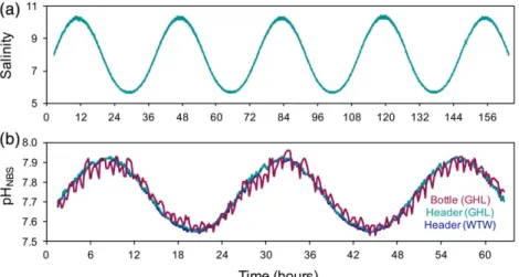
To demonstrate the applicability of the mesocosm system for salinity and pH variability experiments, sinusoidal proﬁles for both parameters were applied. Salinity manipulations of freshening scenarios were done at amplitudes of 2.4 salinity units, above and below mean, with a wavelength of 1.5 d.

Fig. 4.Applied temperature proﬁles of the stochastic regimes run in the mesocosms over 7.5 d as imitations of natural ﬂuctuation patterns recorded in the Kiel Fjord. Treatments were run at ambient (typical for April in Kiel Fjord; purple) or at a warming scenario of +3C (turquoise).

The black lines represent the implemented temperature curves, the col- ored lines show the measured temperatures recorded by the aquarium controllers themselves.

(8)

Salinity values were set with a temporal resolution of 10 min.

Data were logged by the aquarium controllers (GHL, Germany) and additionally by a CTD salinity logger (Star-Oddi, Reykjavik, Iceland), every single minute (Fig. 5A). Manipulations and data recordings were conducted in one of the 600 L mesocosms directly. Aquarium controllers regulated a solenoid valve (M- ventil 1/2⁰⁰, Aqua Medic) connected to a freshwater supply. A constant temperature of 16C was maintained in the system.

Manipulations of pH were applied in December 2016 at amplitudes of 0.2 pHNBS (NBS scale) units above and below mean, and a wavelength of 1 d, reflecting naturally occurring patterns in thefield (Saderne et al. 2013). Nominal pH values were set with a temporal resolution of 30 min. The carbonate system was manipulated inside the header tank, which then supplied a 4.5 L cell culture bottle with aflow rate of 250 mL pre-conditioned seawater per minute. The cylinder was posi- tioned inside a 600 L mesocosm tank that served as a water bath maintaining a constant temperature at 10C. Seawater salinity was 16. The aquarium controller regulated a CO2solenoid valve (GHL, Germany), connected to a constant air-CO2-mix supply of 5000μatm CO2(Bleich et al. 2008). Data (pH) were measured inside the header tank as well as in the 4.5 L cylinder and logged by the aquarium controllers every 8 min (Fig. 5B). In addition, a MULTI 3630 IDS (WTW, Germany) recorded temperature and pH in the header tank every 8 min (Fig. 5B).

Manipulated feeding

Forty eight peristaltic pumps (12 Doser 2.1 Slave, GHL Ger- many) are connected to the aquarium controllers via PAB enabling communication between single pumps. This allows for frequent or constant feeding or for a deﬁned water supply to the EUs (Supporting Information Fig. S4d). Recurrent additions of food (e.g.,Rhodomonassp.) to 48 EUs can be achieved.

If desired, the pumps can also be used for additions of other liquids such as nutrients or suspensions of plastic particles.

Application

KIB Assessment 600 L mesocosms to single EUs

In two separate experiments, in March to April of 2016 (Exp I) and 2017 (Exp II), we evaluated the functionality of mesocosms’ temperature treatments for experiments with single-species (Exp I and Exp II, in small EUs) and communities (Exp II, in the 600 L mesocosms), as well as the application of differing monitoring approaches (from logging devices to hand-held measurements).

Mean warming of the Baltic Sea is projected to range between 3C and 6C until the end of the century (HELCOM 2007; Gräwe et al. 2013). This expectation is corroborated by an observed multi-decadal warming trend in this region of 0.5–1C per decade since the second half of the 20^thcentury (Elken et al. 2015). Predicting future changes of temperature variability and its consequences for marine life is difficult. We have chosen to apply a proof-of-concept setup to demonstrate the power and limitations of the here presented mesocosm system, using sinusoidal fluctuation patterns. The latter provide the advantage to test impacts of temperature deviations from the mean, while organisms experience the same mean temperature conditions, irrespective of frequencies and amplitudes offluctuations. Hence, over the entire duration of the experiments, the species of interest spent an equal cumulative amount of time above and below the mean temperature of a given treatment, but with less and more frequent deviations from this mean. Noticeably, the slopes, i.e., the rates of temperature change differ between treatments of differing frequencies and amplitudes.

Fig. 5.Salinity manipulations are demonstrated as sinusoidal functions over 7 d at amplitudes of 2.4 salinity units above and below mean, and a wavelength of 36 h. Salinity was measured continuously by the aquarium controllers and by external CTD loggers (Star-Oddi, Reykjavik, Iceland;A). The pH manipulations are demonstrated as sinusoidal functions over 2.5 d, at amplitudes of 0.2 pH units above and below mean, and a wavelength of 24 h (B).

Seawater pH was measured continuously by aquarium controllers (GHL, Germany) and repeatedly (every 8 min) with an external MULTI 3630 IDS hand probe, WTW, Germany).

(9)

Temperature manipulations in both experiments were conducted in four treatments over each 7 weeks, withﬂuctuation amplitudes of 2C, above and below mean, and wavelengths of 1.5 d and 4.5 d. Treatments were run with a mean temperature of 5C (representative for winter/spring sea surface temperatures in Kiel Fjord) and at a future-warming scenario of +2C. Thus, “5C, constant” (5Co), “7C, constant” (7Co),

“7C, ﬂuctuating at lowfrequency”(7LF), and “7C,ﬂuctuat- ing athighfrequency”(7HF) treatments were applied (Fig. 6).

The difference between 5Co and 7Co indicates the effect size of the average stress treatment in the absence ofﬂuctuations.

The comparisons between the other treatments (7Co, 7LF, 7HF; all with a mean temperature of 7C) indicate the stress- modulating effects offluctuations and the relative influence of the fluctuation frequency on its capacity to modulate the impact of a driver.

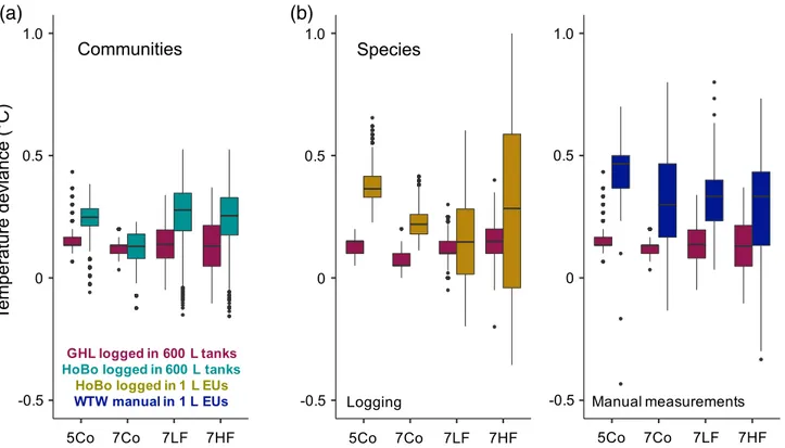
The applied temperatures were monitored using three different sensor types: (1) measurement of temperatures with the aquarium controllers’ temperature sensors (GHL, Germany) and data storage by the aquarium controllers (which also implemented the temperature proﬁles and are thus not independent). For external validation, (2) logging of temperatures by

independent HOBO loggers and (3) by reference measurements using hand-held thermometers (WTW, Germany) were applied.

In Exp I (single species approach), data were logged every 15 min by the aquarium controllers in the mesocosms (n= 2 per treatment level). In addition, three random 1 L Kautex bottles were equipped with HOBO loggers each one per mesocosm (n= 6 per treatment level; at intervals of 15 min). In Exp II (single species and communities), temperature was logged at intervals of 40 min by the aquarium controllers in the mesocosms directly (n= 3). Each mesocosm was further equipped with oneﬂoating HOBO logger placed inside the mesocosms (community approach; n= 3; at intervals of 40 min), yet outside the EUs. Here, reference temperature measurements inside the EUs were done with a hand-held thermometer twice per week (single species approach; n= 9). The EUs received through- ﬂowing seawater from the Kiel Fjord at rates of 12–13 mL per minute.

Biological impacts of temperature variability frequency on mytilid mussels

During Exp I (see above), in addition to the assessment of the mesocosms’ temperature manipulation itself, we assessed Fig. 6.Applied temperature proﬁles during Exp I over 50 d at amplitudes of 2C (above and below mean) and wavelengths of 1.5 d and 4.5 d. Treat- ments were run at ambient temperature (typical for March and April in Kiel Fjord) or at a future-warming scenario of +2C. Set values (black), mean temperature data logged by aquarium controllers in the two parallel mesocosms for each treatment (turquoise lines; means SD [shading];n= 2) and temperature data logged by HOBO loggers directly inside the experimental units (means [yellow]SD [shaded area];n= 5) are presented.

(10)

the relative importance of frequency of temperature ﬂuctua- tions on the performance of the blue mussel, Mytilus edulis (hereafterMytilus).

Individuals of Mytilus were collected in February 2016 at the GEOMAR pier in Kiel, Germany (5419⁰45.97⁰⁰N, 10 8⁰58.58⁰⁰E; at 30 cm water depth). Gently cleaned of fouling organisms, the mussels were kept in a climate chamber with ﬂow-through seawater at 5C until the start of the experiment.

Mussels were 51.01.5 mm (meansSD) in size at the start of the experiment. The experiment was initiated by randomly distributing the mussels into 32 1 L Kautex bottles (EUs), which were distributed among eight 600 L mesocosms (n= 8;

seeSupporting Information Fig. S4b). Subsequently, the mussels were exposed to the four different temperature proﬁles (“5Co,” “7Co,” “7LF,” and“7HF”; see above and Fig. 6) for 50 d. Salinity varied naturally with Kiel Fjord conditions ranging between 13 and 18.

Each EU received flow-through water at a flow rate of 12 mL per min (peristaltic pumps: IPC-N, Cole-Parmer GmbH, Germany) via two separate header tanks (each header tank supplied four of the eight mesocosm units). To feed the mussels, aRhodomonassp. suspension with an average concentration of 1.1× 10⁶ cells mL⁻¹ was supplied to the two header tanks at a flow rate of 162 mL per hour (peristaltic pumps:

IPC-N, Cole-Parmer GmbH, Germany). The header tanks themselves received sand-ﬁltered seawater from Kiel Fjord at a ﬂow rate of 300 mL per min, resulting in a Rhodomonas sp. concentration of approximately 7×10³cells mL⁻¹in the water reaching the EUs (Riisgard et al. 2011). Algal cell counts were determined using a Coulter Counter (Z2 Coulter Particle count and size analyser, Beckman Coulter TM) set to count particles of a size range of 5–8μm. The header tanks and all EUs were aerated to keep algal cells in suspension.

At the start and at the end of the experiment, mussels were measured using a caliper (Wiha dialMax, Schonach, Ger- many). Growth is represented as percent increase in mussel shell length. At the end of the experiment, all mussels were frozen at−20C and stored until further analysis. To measure the mussels’body condition, animals were defrosted, and the soft tissue was manually excised from the shells and dried at 80C for 24 h. Subsequently, dry weights were determined to the nearest mg (0.1 mg; Sartorius, Berlin, Germany). The condition index (CI) of each mussel specimen was calculated from the dry weight of soft tissue and the dry weight of the shell according to the formula: CI = tissue shell-weight⁻¹(mg/mg;

after Mann and Glomb 1978).

For statistical analyses, the software package R was used (R Core Team 2016). Differences between treatment levels were analyzed using ANOVA. The datasets were tested for homogene- ity of variances on the basis of residual plots and the Fligner- Killeen test procedure. Normality of errors was assessed on the basis of histograms of the residuals and the Shapiro–Wilk-W-test and inﬂuential data points using Cook’s distance plots. Post hoc comparisons were achieved using Tukey’s HSD.

Results

Temperature treatments

In both experiments (Exp I and Exp II), the achieved temperature profiles reflected the anticipated treatments (Fig. 6, Supporting Information Fig. S6). For the community approach (Exp II), temperatures were recorded in the mesocosms and aligned the implemented temperature profiles almost perfectly (Supporting Information Fig. S6). However, a constant positive offset of about 0.2C (GHL aquarium controllers; Fig. 7) or 0.3C (HOBO loggers; Fig. 7A) was observed. Hence overall, the temperature treatment levels 5Co, 7Co, 7LF, and 7HF reached mean values of: 5.39C, 7.12C, 7.24C, and 7.25C, respectively (HOBO loggers). This small offset can be mostly attributed to the temperature control system applying a hysteresis of 0.1C. A comparably high surrounding room air temperature of 16C likely also had a small warming effect on the treatment temperatures (with temperatures ranging between 5C and 9C).

For the single-species approach (Exp I and II), data were recorded inside the 1 L EUs and temperatures varied slightly more from set values (Fig. 6, Supporting Information Fig. S6), with positive deviations of about 0.4C (HOBO loggers;

Fig. 7B). The anticipated peaks in temperature ﬂuctuation treatments, were reached appropriately (Fig. 6, Supporting Information Fig. S6). Overall, the four temperature treatments reached mean values of: 5.38C, 7.22C, 7.17C, and 7.27C (as assessed by HoBo loggers, Exp I) in the EUs for the 5Co, 7Co, 7LF, and 7HF treatments, respectively. Hand-held temperature measurements, comparing temperatures in water baths (600 L mesocosm) and the EUs, exhibited deviations on average by +0.41C, +0.31C, +0.34C, and +0.27C (means) in the 5Co, 7Co, 7LF, and 7HF treatments, respectively (Fig. 7B). These offsets can, again, be partly attributed to the temperature control system applying a hysteresis of 0.1C (and thus producing 0.1–0.2C higher values; Fig. 7B). Here, the comparably high room temperature of 16C (treatment temperatures again ranging between 5C and 9C) led to an additional increase of about 0.2C (compared to set values;

Fig. 7B).

The inﬂuence of room temperature on single EUs of different volumes was assessed in addition to the presented experiments from sets of experiments conducted between 2016 and 2018 (Supporting Information Table S1). Temperature deviations between set values and the EUs themselves depended on the volume and shape of the EU utilized in the respective experiment, as well as on the difference between treatment and room temperature. Deviations from set values were within 0.25C standard deviation of the mean, and generally increased with increasing difference of treatment and room temperature (Supporting Information Fig. S7). Overall, signiﬁ- cant day/night temperature patterns could not be observed, likely because the LED light bars emit relatively little heat to the system (Fig. 6, Supporting Information Fig. S6).

(11)

Mussel responses to temperature treatments

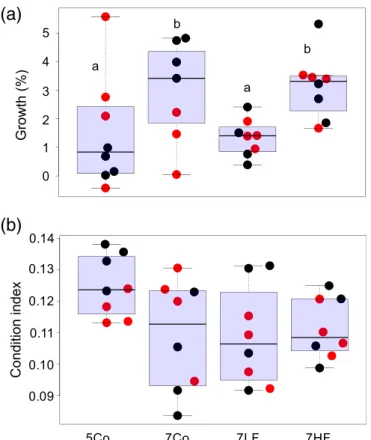
The frequency of temperature fluctuations significantly influencedMytilusgrowth rates: Mussels grew 134% faster in the 7HF treatment compared to the 7LF treatment. However, similar growth rates between the 7HF treatment and 7Co treatment (F3= 3.268,p= 0.0365; Fig. 8A) were observed. The condition index of mussels was very variable between individuals and not significantly affected by the applied treatments (adults:F3= 2.493,p= 0.0805; Fig. 8B). In the 5Co treatment, the average condition of mussels tended to be slightly better than in the other treatments. Tank effects were not observed for growth (Fig. 8A; ANOVA on tanks:p= 0.7090), or for the condition index of mussels (Fig. 8B; ANOVA on tanks:

p= 0.5155).

Discussion

Worldwide, so far only very few mesocosm systems were designed for replicated and longer-term (> weeks to few months) studies on marine benthic systems in medium to large-scale experimental units (> 500 L; partly reviewed in Stewart et al. 2013; Wahl et al. 2015). In the tropic and sub- tropic zones, the SeaSim facility in the Australian Institute for

Marine Sciences in Townsville, Queensland, Australia (https://

www.aims.gov.au/seasim), the mesocosm facility at the South Australian Research and Development Institute (SARDI) Aquatic Sciences, West Beach, Australia (Falkenberg et al.

2016), a mesocosm system on Hawaii (Jokiel et al. 2014), the CRETACOSMOS at the Hellenic Centre for Marine Research in Greece, the Red Sea Simulator (Bellworthy and Fine 2018), or the Coral Vivo Project Research Station in Brazil (Duarte et al.

2015), were established - mainly for temperature and pH manipulations in either static or real-time offset ((Duarte et al. 2015);

maintaining ﬁeld variability) treatment approaches. Some of these systems can also expose organisms or communities to local environmental stressors such as nutrients or contaminants (Duarte et al. 2015), or differing light conditions, salinity shifts, and/or sedimentation (SeaSim, Australia). In temperate latitudes, the Kiel Outdoor Benthocosms in the Baltic Sea (Wahl et al.

2015) and the Sylt Benthic Mesocosm Facility (Pansch et al.

2016) in the North Sea (Wadden Sea) were recently established, mainly testing temperature and acidiﬁcation (partly eutrophication) effects on communities. The Baltic Hard Bottom Meso- cosms (BHB-mesocosms), a land-based outdoor enclosure system, mainly tested impacts of efﬂuents (Kraufvelin 1998).

Other temperate benthic marine mesocosm infrastructures are

(a) (b)

Fig. 7.Temperature deviations from set values in the 600 L mesocosm tanks (community approach;A; Exp II) and in 1 L Kautex bottles (single-species approach;B; Exp I and II; see Fig. 6, Supporting Information Fig. S6 for entire temperature proﬁles). Treatments consisted of constant temperatures at 5 (5Co) and 7C (7Co), as well as temperatureﬂuctuations around 7C with amplitudes of 2C above and below means, and wavelengths of 1.5 (7HF) and 4.5 (7LF) days. Measurements were done with the use of HoBo loggers in the mesocosms (A; turquoise) or in the 1 L Kautex bottles directly (B; yellow), as well as with the use of a handheld thermometer directly inside the 1 L Kautex bottles in comparison to the mesocosm tank temperatures (B;

blue). Temperature deviations from set values recorded by the aquarium controllers in the respective experiments are presented in purple. Data are presented as boxplots (median, upper, and lower quartile (75^th/25^thpercentile), whiskers (1.5 times the interquartile range, outliers).

(12)

the Solbergstrand Experimental Facility at the Norwegian Insti- tute for Water Research, Norway (www.aquacosm.eu/) or the Plymouth Marine Laboratory Mesocosms (www.pml.ac.

uk/facilities/mesocosm). The large capacities (volumes) of these mesocosm systems usually allow for community-level studies.

However, their large size typically limits replication and/or multi-driver experimentation (Stewart et al. 2013). Yet, to the best of our knowledge, no mesocosm facility was established to test the consequences from environmental variability on single species to entire communities.

The Kiel Indoor Benthocosms (KIBs)

On the basis of empirical mesocosm studies in terrestrial systems (Bestion et al. 2015; Yvon-Durocher et al. 2015), Fordham (2015) emphasized why mesocosm experiments truly emerge as powerful tools for identifying the ecological processes that drive population- and community-level responses to climate change, as well as for testing fundamental principles in ecology. Hence, a more robust knowledge of community-level

effects and also of their underlying explanatory variables (often single-species effects) is needed. We therefore suggest the application of a novel experimental platform that enables experiments on single-species and communities, the Kiel Indoor Benthocosms (KIBs).

The major—and novel—feature of the KIB facility is the capacity to simulate environmental variability as real-time offsets or as any programmed fluctuation regime of multiple drivers (temperature, salinity, pH, light intensity). Data monitoring and alarm notification further allow for reliable and up- to-date long-term experiments at reduced labor intensities. In addition, the KIB system is less costly (altogether approximately 60k €) than most outdoor systems. KIBs are located indoors in a constant temperature room, allowing for independence from highly variable and non-predictive sunlight irradiation, and air temperature variability. It does not only allow for constant light conditions during e.g., incubations of autotrophic organisms, but also for the simulation of differing irradiance regimes, as well as variability in light conditions. At the same time, theflow-through of natural Kiel Fjord seawater, matches seawater parameters (unless intentionally manipulated). Thus, the KIBs represent a unique mesocosm infrastructure for testing the effects from environmental variability of multiple drivers on species and communities in benthic temperate systems.

Performance of the KIBs’temperature treatments: from mesocosms to EUs

With the demonstrated assessment examples, we highlight the applicability of the KIBs for species (in experimental (sub-) units, EUs) as well as community (in 600 L mesocosms) approaches. Target systems tested in the KIBs to date were both, single benthic species (e.g.,Mytilus edulis,Clupea haren- gus [benthic eggs], Asterias rubens, Balanus improvisus, Hemi- grapsus takanoi,Littorina littorea, Electra pilosa) and simpliﬁed communities (e.g., Fucus vesiculosus with Gammarus sp. and Idotea baltica grazers), testing the effects from short-term or seasonal temperatureﬂuctuations, as well as diurnal pH variability. Experimental time frames ranged from weeks to several months.

During temperature simulations and two 50-d experiments (Exp I and II), temperature conditions were monitored in smaller EUs of 1 L (placed inside the mesocosms) or in the 600 L mesocosms directly, simulating single-species or community approaches, respectively. Temperature treatments ranged from constant and sinusoidal to stochastic - shortly changing - conditions. The observed temperatures reflected the implemented treatment conditions extremely well, particularly so in the 600 L mesocosms. When working in smaller EUs of 1–18 L (i.e., a water-bath approach), surrounding room temperatures, temperatures of incoming Kiel Fjord seawater (in a flow-through approach), as well as flow rates into the smaller units, all, impacted the accuracy of the treatment temperatures in the EUs. Heat exchangers are proposed to

(a)

(b)

Fig. 8.Temperature effects onMytilus edulisover 50 d at constant temperatures at 5 (5Co) and 7C (7Co), as well as temperatureﬂuctuations around 7C with amplitudes of 2C above and below means, and wavelengths of 4.5 (7LF) and 1.5 (7HF) days. Size increments of mussels (in percent) from start and end measurements of mussel lengths (A), as well as the condition index (B) are shown. Data are presented as boxplots (median, upper, and lower quartile (75^th/25^th percentile), whiskers (1.5 times the interquartile range, outliers) and as real data points representing mesocosm A (black) or B (red;n= 8). Signiﬁcant differences are indicated by lower case letters (Tukey’s HSD).

(13)

overcome the variability and deviance in incoming seawater.

Particularly strong differences between room temperatures and treatment temperatures in the tanks, mostly at peaks of ﬂuctuation patterns, presented the main factor inﬂuencing the accuracy of treatment temperatures inside the single EUs.

This can partly be overcome by adjustments in room temperatures during the experiments (preferably to mean treatment temperatures). Recordings of environmental data using commercially available data loggers as well as discrete manual measurements, as suggested herein, will aid the evaluation of true offsets from target treatment conditions and therefore allow for reliable interpretation of results.

Effects of frequency in temperature variability on mussels In a 50-d experiment on the ecosystem engineer Mytilus edulis (Borthagaray and Carranza 2007), this study demonstrated that not only changes in means and the variability of temperature, but also in the frequency of aﬂuctuating temperature regime can be of importance for an organisms’ performance. Implemented constant temperature regimes showed, not surprisingly (Larsen et al. 2014), that an increase in overall mean temperature led to an increase in mussel growth. Thus, mussels were able to obtain enough food to fuel their ther- mally increased metabolic activity at increased temperatures, in agreement with (Fly et al. 2015). The condition of mussels was not impacted by the applied temperature treatments.

Most interestingly, an impact of the frequency of temperature ﬂuctuations was detected on Mytilus growth. To our knowledge, this has not been demonstrated before, and calls for a deeper assessment of the underlying mechanisms.

Within the framework of Jensen’s inequality, any variation around a mean driver should affect the performance of an organism, when compared to constant conditions (Ruel and Ayres 1999). Here, the effect fundamentally depends on the shape of the organisms’temperature performance curve (TPC), as well as on the respective position along the TPC at which the treatment temperature is applied (Ruel and Ayres 1999;

Sinclair et al. 2016). In mytilid mussels (and most other organisms), considering the applied low temperatures of the present study (Fly et al. 2015; Sinclair et al. 2016), temperature variability around 7C should have increased mussel performance when compared to constant conditions at the same mean (fol- lowingJensen’s inequality). However, this was not true for temperature variability of any frequency. In contrast, temperature variability of low-frequency reduced the performance of mussels in the present study, compared to constant and high- frequency conditions with the same mean temperature. Possi- bly, at increased and slowlyﬂuctuating temperatures, periods with unfavorable (low) temperatures were too long, during which Mytilus could not compensate for periods of more favorable (warmer) condition (as suggested in Wahl et al.

2016). Underﬂuctuations with higher frequency, low temperature periods represented only a short excursion into cold water, which overall did not negatively affect mussel growth.

This also supports the hypothesis that temperature is growth limiting, particularly so at temperatures below 7C. Further detailed assessments of the mussel physiology seem to be necessary to explain this observation, using systems such as the KIBs.

Relevant experimentalﬂuctuation treatments

Environmental factors such as temperature, salinity, pH, light, and oxygen can ﬂuctuate at various modes with differing intensities and frequencies (see Supporting Information Fig. S1 for temperature variability, see also Boyd et al. 2016).

In the past, research on mean changes in environmental drivers was based on well-established ocean models (Rhein et al. 2013; Pörtner et al. 2014). However, predictive models for changes in environmental variability are limited (Bates et al. 2018). Extreme events, as only one asset of the many scales at which ﬂuctuations can occur, are projected to increase in intensity and frequency (Perkins et al. 2012). Still, to date, few models (but see Kowch and Emanuel 2015) elucidate the extent to which this will occur (see discussions in Boyd et al. 2016; Hobday et al. 2016). Frölicher et al. (2018) projects the duration of heatwaves to increase by a factor of 41 under 3.5C mean warming scenario, with a spatial extent that is 21 times larger than in preindustrial times. This information is valuable and can be implemented into ecological experiments. Little to no information, however, is available from regional models and on changes in smaller-scale variability patterns, as well as multiple drivers (Bates et al. 2018).

Almost no information exists on the effects of such increased climatic variability on marine species (but see Morash et al.

2018) and communities. Here, the KIBs were proven to simulate fluctuations at various amplitudes and frequencies, and also to simulate stochastic natural events retrieved from the field. Furthermore, serving as aproof-of-concept, in the present study the effects of sinusoidalfluctuation regimes on mussel performance were successfully tested. The KIB system, therefore, can help bridge knowledge gaps (Morash et al. 2018) on the effects of shiftingfluctuation regimes in the marine realm.

Further applications and future perspectives

In the present conﬁguration the KIBs are in a developmen- tal stage at which already many pressing research questions can be addressed, from single species to the community level, from sinusoidal and stochasticﬂuctuations to extreme events and in short- to long-term experiments. With temperature in focus, this is currently the central agenda of the KIBs. The out- comes will give many new insights into the effects of environmental variability on coastal benthic marine ecosystems.

While the exemplifying study on mytilid mussels (and most assessments in the KIBs) presented in this article focuses on temperature variability, salinity, and pH ﬂuctuations are also shown to be successfully simulated at improved and therefore more realistic diurnal sinusoidal, near-natural modes in the KIB system (see e.g., Cornwall et al. 2013 for comparisons).

(14)

Light variability and/or pollution from night-time light can also have strong impacts on coral physiology and ecology (Kaniewska et al. 2015). However, light pollution was not the focus of the present study and earlier investigations. Nutrient conditions or plastic particle additions may also be manipulated by frequent dosing events using the installed peristaltic pumps. Tidal rhythms are not included in the performance of the KIB system due to the lack of tides in Baltic Sea habitats. Wave generators, are not part of the current setup, either, but can be achieved by the use of commercially available aquarium wave generating pro- peller pumps.

At present, the KIB infrastructure and experiments have focused on conceptual frameworks (sinusoidalﬂuctuations). In future investigations, the focus will be shifted toward simulating extreme events (i.e., marine heatwaves [Hobday et al.

2016]). Here, approaches as previously demonstrated in Pansch et al. (2018) may be applied. This assures near-natural stochastic temperature variability, while changing the parameter of interest: an extreme temperature event in this speciﬁc example.

In addition, coastal systems are particularly prone toﬂuctua- tions of many factors (e.g., Feely et al. 2008; Duarte et al. 2013;

Waldbusser and Salisbury 2014), which, may interact (Vajed Samiei et al. 2016; Reusch et al. 2018). Extreme events such as upwelling, may, depending on season, include cooling of water masses, hypoxia, a drop in seawater pH (with accompanied changes in carbonate chemistry) as well as an increase in salinity and/or nutrients (Melzner et al. 2013). In this context,ﬂuc- tuations of different parallel drivers and their interactions must be considered in future investigations (Boyd 2011; Riebesell and Gattuso 2015; Pendleton et al. 2016; Brennan et al. 2017).

The recent development of autonomous incubation chambers, which can be applied in the KIB mesocosm system, allows for conducting highly controlled—but natural—climate change community experiments. Units with a set of comple- mentary sensors (pH, salinity, temperature, nutrients, etc.) will allow for online monitoring of biological responses of communities (community respiration and O2production) under various constant or ﬂuctuating scenarios. Measured at high frequency such community responses may elucidate whether organisms can make use of certain time windows for recovery or higher performance such as increased photosynthesis, respiration, or calciﬁcation (Wahl et al. 2018).

Conclusions

Humans have persistent impacts on coastal marine ecosystems and the goods and services they provide. Taken that climate change research can only predict future ecosystem shifts from more advanced studies by up-scaling from species to ecosystems, from single to multiple drivers, and from short-term to long term incubations (Riebesell and Gattuso 2015), there is an urgent need to extend these anticipated research efforts by including the concept of environmental ﬂuctuations (Neilan and Rose 2014; Gunderson et al. 2016; Wahl et al.

2016; Bates et al. 2018; Morash et al. 2018). For the marine realm, diverse approaches, ranging from small-scale laboratory experiments to mesocosms, FOCE systems (Gattuso et al.

2014) and field observations have been established over the decades, each of which provide their own benefits (Stewart et al. 2013). The sum of all of these approaches will greatly advance our understanding of species, communities, and ecosystems in a changing world. However, to the best of our knowledge, to date, no mesocosm systems were established with the focus of testing the impacts of variability of environmental drivers on marine species or communities. This study demonstrates that temperature variability, but more importantly, the frequency offluctuation patterns, mediates global change impacts on a key marine species. Thus, the Kiel Indoor Benthocosms (KIBs) provide a new approach for elucidating the role of natural environmental variability as an amplifier or buffer of ecosystem change in single species and communities, thereby providing a large potential to better explain and predict future ecosystem shifts in shallow marine habitats.

References

Andersson, A. J., and others. 2015. Understanding ocean acid- ifcation impacts on organismal to ecological scales. Ocean- ography28: 16–27. doi:10.5670/oceanog.2015.27

Bates, A. E., and others. 2018. Biologists ignore ocean weather at their peril. Nature Comment (London) 560: 299–301.

doi:10.1038/d41586-018-05869-5

Bellworthy, J., and M. Fine. 2018. The Red Sea Simulator: A high-precision climate change mesocosm with automated monitoring for the long-term study of coral reef organisms.

Limnol. Oceanogr.: Methods 16: 367–375. doi:10.1002/

lom3.10250

Bestion, E., A. Teyssier, M. Richard, J. Clobert, and J. Cote.

2015. Live fast, die young: Experimental evidence of population extinction risk due to climate change. PLoS Biol.13: e1002281. doi:10.1371/journal.pbio.1002281

Bleich, M., and others. 2008. Kiel CO2 manipulation experimental facility (KICO2). Second Symposium on the Ocean in a High-CO2 World. doi:10.13140/2.1.3818.0809

Bleich, S., M. Powilleit, T. Seifert, and G. Graf. 2011. Beta- diversity as a measure of species turnover along the salinity gradient in the Baltic Sea, and its consistency with the Ven- ice System. Mar. Ecol. Prog. Ser. 436: 101–118. doi:

10.3354/meps09219

Borthagaray, A. I., and A. Carranza. 2007. Mussels as ecosystem engineers: Their contribution to species richness in a rocky littoral community. Acta Oecol. 31: 243–250. doi:

10.1016/j.actao.2006.10.008

Boyd, P. W. 2011. Beyond ocean acidiﬁcation. Nat. Geosci. 4: 273–274. doi:10.1038/ngeo1150

Boyd, P. W., C. E. Cornwall, A. Davison, S. C. Doney, M.

Fourquez, C. L. Hurd, I. D. Lima, and A. McMinn. 2016.