Meso- and submesoscale
variability within the Peruvian upwelling regime: Mechanisms
of oxygen supply to the subsurface ocean.
Dissertation
zur Erlangung des Doktorgrades
der Mathematisch - Naturwissenschaftlichen Fakult¨ at
der Christian-Albrechts-Universit¨ at zu Kiel
vorgelegt von
S¨ oren Thomsen
Kiel, Dezember 2015
Erster Gutachter: Prof. Dr. Torsten Kanzow
Zweiter Gutachter: Prof. Dr. Richard J. Greatbatch
Tag der m¨undlichen Pr¨ufung: 05.02.2016 Zum Druck genehmigt: 05.02.2016
gez.
Prof. Dr. Wolfgang J. Duschl, Dekan
F¨ur dich Klaus
Abstract
The role of meso- and submesoscale processes for the near-coastal circula- tion, physical and biogeochemical tracer distributions and oxygen minimum zone ventilation in the Peruvian upwelling regime is investigated in this the- sis. A multi-platform four-dimensional observational experiment was carried out off Peru in early 2013 and is the basis for this thesis. Furthermore a high-resolution submesoscale permitting physical circulation model is used to study submesoscale frontal dynamics in more detail. The formation of a sub- surface anticyclonic eddy and its impact on the near-coastal salinity, oxygen and nutrient distributions was captured by the observations. The eddy de- veloped in the Peru-Chile Undercurrent downstream of a topographic bend, suggesting flow separation as the eddy formation mechanism. The eddy resulted in enhanced cross-shore exchange of physical and biogeochemical tracers due to along-isopycnal stirring and offshore transport of core waters.
The core waters originated from the bottom boundary layer and were char- acterized by low potential vorticity and an enhanced nitrogen-deficit. The subduction of highly oxygenated surface water in a submesoscale cold fila- ment is observed by glider-based measurements. The subduction ventilates the upper oxycline but does not reach into oxygen minimum zone core wa- ters during the summer observations. Lagrangian floats are used to study the pathways of newly upwelled water in a regional submesoscale permit- ting model. The model analysis suggests a gradual warming of the newly upwelled waters due to surface heat fluxes. The associated density decrease prevents the floats to enter the density range of the oxygen minimum zone in summer. However, in winter a density increase is found due to surface cool- ing and thus it might be possible that submesoscale processes ventilate the oxygen minimum zone. In the model about 50 % of the newly upwelled floats leave the mixed layer within 5 days both in summer and winter emphazising a hitherto unrecognized importance of subduction for the ventilation of the Peruvian oxycline.
Zusammenfassung
Ziel dieser Doktorarbeit ist es zu einem tieferen Verst¨andnis f¨ur die Rolle von meso- und submesoskaligen Prozessen f¨ur die Zirkulation, die physikalis- chen und biogeochemischen Tracerverteilungen sowie die Sauerstoffventila- tion in der k¨ustennahen Sauerstoffminimumzone vor Peru beizutragen. Hi- erf¨ur wurde eine auf verschiedenen Plattformen basierende vier-dimensionale Messkampagne im Fr¨uhjahr 2013 vor Peru durchgef¨uhrt. Zus¨atzlich wurde ein hochaufl¨osendes physikalisches Ozeanzirkulationsmodel, welches Bereiche des submesoskaligen Regimes explizit aufl¨ost, genutzt um submesoskalige Frontenprozesse im Detail zu untersuchen. Die Formation eines antizyk- lonalen Wirbels mit Kern unterhalb der Thermokline und dessen Einfluss auf die k¨ustennahe Salz-, Sauerstoff- und N¨ahrstoffverteilung konnte w¨ahrend der Messkampange beobachtet werden. Da sich der Wirbel direkt hinter einer abrupten topographischen Biegung bildet, wird Str¨omungsabl¨osung als Wirbelformationsmechanismus vermutet. Auf Grund von mesoskaliger Vermischung entlang von Isopykanen und dem Transport von Wasser im Wirbelkern verursacht der Wirbel einen erh¨ohten Austausch von physikalis- chen und biogeochemischen Tracern zwischen dem offenen Ozean und der K¨ustenregion. Die Kernwassermassen entstammen der bodennahen turbu- lenten Grenzschicht und zeichnen sich durch niedrige potentielle Wirbel- haftigkeit sowie erh¨ohten Stickstoffmangel aus. Die Subduktion von mit Sauerstoff angereichertem Oberfl¨achenwasser innerhalb eines submesoskali- gen Kaltwasserfilaments wurde von Gleitermessungen aufgezeichnet. Die Subduktion ventiliert die obere Oxykline, reicht allerdings im Sommer nicht bis in den Kern der Sauerstoffminimumzone. Mit Hilfe von numerischen Lagrangschen Partikeln wird der Pfad von frisch aufgetriebenem Wasser in einem regionalen Ozeanmodel, welches submesoskalige Prozesse teilweise ex- plizit aufl¨ost, untersucht. Die Modeluntersuchungen lassen vermuten, dass eine kontinuierliche Erw¨armung des aufgetriebenen Wasser erfolgt. Die damit verbundene Reduzierung der Dichte hindert die Partikel im Sommer in den Dichtebereich der Sauerstoffminimumzone zu gelangen. Im Winter hingegen wird teilweise eine Erh¨ohung der Dichte durch atmosph¨arische Abk¨uhlung beobachtet, welche eine Ventilation der Sauerstoffminimumzone durch sub- mesoskalige Prozesse erm¨oglichen k¨onnte. Im Model verlassen ungef¨ahr 50 % der frisch aufgetriebenen Floats die Deckschicht innerhalb von 5 Tagen. Dies deutet auf eine bis dahin unerkannte Wichtigkeit von Subduktionsprozessen f¨ur die Ventilation der peruanischen Oxykline hin.
Contents
1 Introduction 1
2 Theoretical background 6
2.1 Definition of key terms . . . 6
2.1.1 Richardson and Rossby number . . . 6
2.1.2 Rossby and mixed layer radius . . . 6
2.1.3 Oceanic fronts . . . 7
2.1.4 Geostrophic balance . . . 7
2.1.5 Potential vorticity and symmetric instability . . . 8
2.2 Mesoscale dynamics . . . 9
2.3 Submesoscale frontal processes . . . 10
2.4 Frontogenesis and cold filamentary intensification . . . 13
2.5 Internal waves and three-dimensional microscale turbulence . . 14
2.6 Submesoscale routes to dissipation . . . 15
2.7 Turbulent tracer fluxes in the upper ocean . . . 18
2.8 Physical-biogeochemical coupling in meso- and submesoscale flows . . . 19
3 Observational and model data 22 3.1 Multi-platform observational study in the Peruvian upwelling regime . . . 22
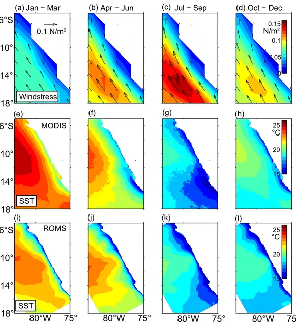
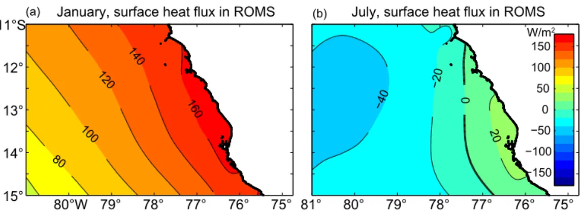
3.2 Regional model simulation of the Peruvian upwelling regime . 22 4 Seasonal cycle of the Peruvian upwelling regime 23 4.1 Wind forcing, surface heat fluxes and sea surface temperature distribution . . . 23
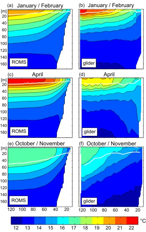
4.2 Cross-shore temperature distribution . . . 27
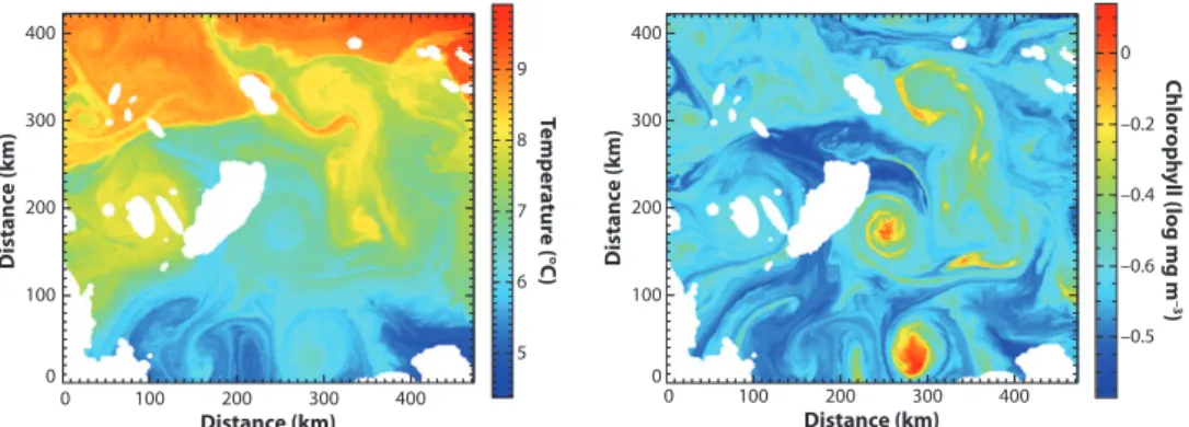
4.3 Submesoscale variability . . . 29
4.4 Summary . . . 30
5 The formation of a subsurface anticyclonic eddy in the Peru- Chile Undercurrent and its impact on the near-coastal salin- ity, oxygen and nutrient distributions 31 5.1 Introduction . . . 31
5.2 Data and methods . . . 35
5.3 Results . . . 40
5.3.1 Oceanographic setting . . . 40
5.3.2 Eddy formation . . . 42
5.3.3 Potential vorticity and eddy generation mechanism . . 43
5.3.4 Impact of the horizontal circulation on the distribu-
tions of salinity and oxygen . . . 48
5.3.4.1 Formation of isolated oxygen patches by ad- vection along isopycnals in a vertically sheared flow prior to the eddy formation . . . 52
5.3.4.2 Formation of small scale salinity and oxy- gen structures by mesoscale stirring after the eddy formation . . . 55
5.3.4.3 Eddy-driven ventilation of the near-coastal oxygen minimum zone . . . 57
5.3.5 Impact of the horizontal circulation on the distribu- tions of nitrate, nitrite and nitrogen-deficit . . . 58
5.4 Discussion . . . 60
5.5 Summary and conclusions . . . 63
6 Do submesoscale processes ventilate the oxygen minimum zone off Peru? 66 6.1 Introduction . . . 66
6.2 Observational and model data . . . 67
6.2.1 Glider and satellite observations . . . 67
6.2.2 Regional ocean model . . . 69
6.3 Results . . . 70
6.3.1 Observed subduction of surface water in a submesoscale cold filament . . . 70
6.3.2 Modeled subduction of newly upwelled water . . . 72
6.4 Discussion and conclusion . . . 75
7 Summary and Synthesis 78 7.1 How is the near-coastal circulation influenced by meso- and submesoscale motion? . . . 78
7.2 How do meso- and submesoscale processes impact on the near- coastal tracer distribution? . . . 80
7.3 What is the role of meso- and submesoscale processes for the ventilation of the near-coastal OMZ off Peru? . . . 81
8 Conclusion 84
9 Future work 85
1 Introduction
The ocean, as an important component of the Earth’s climate system, stores and transports heat, freshwater and climate relevant gases such as CO2 (Siedler et al., 2001). In both the atmosphere and the ocean, turbulent motion drives a large portion of these transports and thus is crucial for the overall climate system (Wunsch, 2002; Zhang et al., 2014). In the ocean turbulent processes exist on various length scales (Olbers et al., 2012). They range from mesoscale eddies with diameters of hundreds of kilometres down to internal waves with wavelength of centimeters which break and stimulate diapycnal mixing on millimeter scales.
In the ocean, turbulent motion has traditionally been categorized into three dynamical regimes: the two-dimensional geostrophic mesoscale, the in- ternal wave field and the three-dimensional microscale (Ferrari and Wunsch, 2009). In recent years, this traditional dynamical view of three exclusive types of motions was expanded by including a fourth regime of motion: sub- mesoscale frontal processes. The latter play an important role in the near surface ocean dynamics, where the geostrophic balance, which holds if the horizontal pressure gradient force is balanced by the Coriolis force, breaks down and ageostrophic effects become important (Thomas et al., 2008; Fer- rari, 2011; Levy et al., 2012). Submesoscale frontal processes are most pro- nounced in the weakly stratified mixed layer but also affect the dynamics within the thermocline (Badin et al., 2011; Ramachandran et al., 2014).
These processes can drive large vertical velocities and thus are crucial for understanding tracer fluxes between the atmosphere and the ocean interior (Capet et al., 2008a). Furthermore submesoscale instabilities seem to provide key mechanisms to connect the three traditional regimes by extracting energy from the balanced geostrophic motion and supplying it to three-dimensional turbulence, where it finally dissipates (Taylor and Ferrari, 2009; Molemaker et al., 2010; Brueggemann and Eden, 2014).
The first idealized basin scale two-layer ocean model with mesoscale ed- dies was developed by Holland and Lin (1975a,b). Since more than 20 years mesoscale eddies are found in more realistic basin scale three-dimensional ocean models (e.g. Treguier et al., 2005) and nowadays there are even high- resolution global climate models which allow the explicit simulation of meso- scale eddies in the ocean (Delworth et al., 2012). However, submesoscale processes are far from being resolved in large-scale long-term simulations (Fox-Kemper et al., 2011). As submesoscale frontal processes are known to be important for air-sea gas exchange, and thus for the fluxes of climate relevant gases, such as CO2 (D’Asaro et al., 2011;Ferrari, 2011), parameter- izations of the effects of subgridscale processes are needed (Fox-Kemper and
Ferrari, 2008;Brueggemann and Eden, 2014). Still there are large uncertain- ties concerning the understanding and the ability to parameterize the effects of submesoscale variability (Mahadevan et al., 2010;Brueggemann and Eden, 2014). Consequently, the uncertainties influence the predictability of quanti- ties that are highly affected by the submesoscales, as e.g. mixed layer depth or the air-sea gas exchange of heat and trace gases (Oschlies, 2002; D’Asaro et al., 2011; Ferrari, 2011). In order to constrain new parametrizations and improve or evaluate the existing ones, a deeper process understanding is needed. However, the recent increase in computational power and the large cost reduction of computing time made it possible to increase the resolution of regional ocean general circulation models down to some hundred meters.
Consequently, more and more high resolution regional and idealized model studies exist that have sufficient resolution to permit submesoscale frontal processes (Thomas et al., 2008; Gula et al., 2014; Molemaker et al., 2015).
The simulations are restricted to certain regions and are only integrated over short time periods of several years. Still they can be used to improve our recent understanding of submesoscale dynamics. However, due to their short integration time the simulations do not capture long term climate signals and thus cannot be used for climate predictions.
Submesoscale processes are characterized by short time scales of O(day) and length scales of O(100 m - 10 km) and thus are hard to capture synop- tically by traditional shipboard measurement programs. Hydrographic mea- surements are able to achieve a vertical resolution of several centimeters but seldom are made closer than ten km apart in the horizontal during large scale surveys. However, if strong lateral density gradients exist and stratification is low, the occurrence of submesoscale processes can be expected. First mea- surements of fronts in the surface mixed layer reach back to the early cam- paigns ofUda (1938),Cromwell and Reid (1956) andKnauss (1957). Despite these early observations the scientific interest in surface fronts is a relatively new phenomenon (Munk et al., 2000;Thomas et al., 2008). This might be re- lated to the fact that the observations of submesoscale near-surface processes increased significantly in recent years due to the developement of towed sys- tems, which enable to measure hydrographic properties with high horizontal resolution (e.g. Pollard and Regier, 1992; Rudnick and Luyten, 1996; Lee et al., 2006; Hosegood et al., 2006; Thomas et al., 2013). Nevertheless, it remains extremely challenging to explore the temporal variability of these small scale processes by direct measurements.
However, new measurement platforms such as gliders are able to capture these processes. Although gliders are relatively slow compared to towed ship- board measurements, they are highly suited to study submesoscale dynamics as they can be used in fleets to achieve three-dimensional fields of variables.
78°W 77° 76°
15°
14°
13°
12°S
18 19 20 21 22
78° 77° 76°
−0.5 0 0.5 1 1.5
Sea surface temperature Surface chlorophyll concentration ln (mg Chl/m3)
°C
b c
96oW 90oW 84oW 78oW 72oW 66oW 20oS
15oS 10oS 5oS
0o
µ mol/kg
0 20 40
a
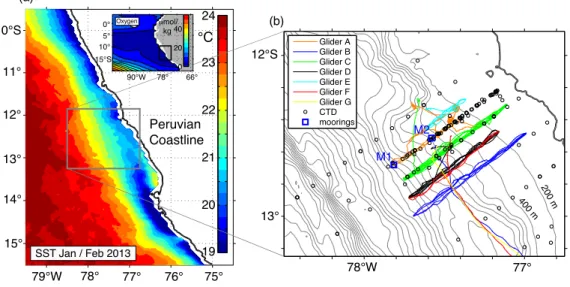
Oxygen
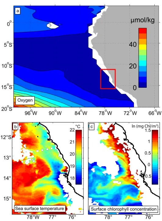
Figure 1: Oxygen concentration (a) inµmol/kg in the eastern tropical Pacific at σθ = 26.8kg/m3 as obtained from the MIMOC climatology (Schmidtko et al., 2013). The red square indicates the region shown in (b) and (c), which represent the study area of this thesis. Sea surface temperature in◦C (b) and surface chlorophyll concentrations (c) in logarithmic form (of unit mg/m3) from MODIS Aqua satellite measurements on January 25 2013 off Peru.
One important challenge due to the short time scale of these processes is to separate temporal and spatial variability, which is difficult with one single moving sensor platform such as a ship alone. However, with a swarm of gliders covering a small area it might become possible to separate spatial from temporal changes.
The Peruvian upwelling regime, as one of the four major eastern bound- ary upwelling systems, shows pronounced meso- and submesoscale variability (Fig. 1b,c; Capet et al. 2008b; McWilliams et al. 2009). Mesoscale eddies and submesoscale filemants have large effects on the horizontal and vertical transport of momentum, heat and tracers (Klein and Lapeyre, 2009). In upwelling systems, this variability is thought to induce a net reduction of bi- ological productivity by exporting nutrients from the productive near-coastal region into the open ocean (Rossi et al., 2008, 2009; Lathuili`ere et al., 2010;
Gruber et al., 2011;Nagai et al., 2015).
The highly productive Peruvian upwelling regime encompasses the most intense and shallowest oxygen minimum zone (OMZ) in the ocean (Fig. 1a;
Karstensen et al.2008;Fuenzalida et al.2009;Paulmier and Ruiz-Pino2009).
OMZs are characterized by a sluggish mean circulation and thus mesoscale eddies are important for ventilating OMZs by means of along-isopycnal stir- ring (Wyrtki, 1962; Luyten et al., 1983a; Stramma et al., 2010; Hahn et al., 2014; Brandt et al., 2015). However, so far little is known about the role of mesoscale eddies for the circulation and ventilation of the near-coastal OMZ off Peru. Submesoscale frontal processes can drive large vertical velocities and enhance vertical tracer fluxes in the upper ocean (Capet et al., 2008a).
Due to the vicinity of the well-oxygenated mixed layer and the OMZ waters below, vertical advective motion driven by submesoscale frontal dynamics might be a key process for the vertical supply of oxygen into the OMZ off Peru. However, submesoscale processes and in particular their potential role for the oxygen ventilation have not been addresses so far.
The focus of this thesis lies on turbulent motion found in the upper ocean in the Peruvian upwelling regimes. In particular the role of meso- and sub- mesoscale processes for the near-coastal circulation, tracer distribution and ventilation of the OMZ is investigated. The following three main scientific questions will be addressed:
1. How is the near-coastal circulation influenced by meso- and subme- soscale motion?
2. How do meso- and submesoscale processes impact on the near-coastal tracer distribution?
3. What is the role of meso- and submesoscale processes for the near- coastal oxygen ventilation?
To answer these questions a multi-platform four-dimensional observational experiment was carried out off Peru in early 2013 which is the basis for this thesis. Furthermore a high-resolution submesoscale permitting physical model is used to study submesoscale frontal dynamics in more detail.
This thesis is structured as follows: First the theoretical background is given in section 2. This includes the definition of key terms used in this thesis (section 2.1). Then follows the introduction of four different oceanic regimes and the underlying physics, including mesoscale dynamics (section 2.2), submesoscale frontal processes (section 2.3 and 2.4) as well as the inter- nal wave and the three-dimensional turbulent regime (section 2.5). The role of submesoscale frontal processes for the energy cycle are described in section 2.6. In section 2.7 the mathematical framework for turbulent tracer fluxes is introduced. The role of meso- and submesoscale flows for the biogeochem- istry is described in section 2.8. The observational dataset and the model simulation used in this thesis are briefly introduced in section 3. The seasonal cycle of the Peruvian upwelling regime is described in section 4. Section 5 consists of a manuscript which is under review for Journal of Geophysical Research - Oceans. The manuscript focuses on the formation of a subsurface anticyclonic mesoscale eddy in the Peru-Chile Undercurrent and its impact on the near-coastal salinity, oxygen and nutrient distributions. In section 6 the question whether submesoscale processes ventilate the oxygen minimum zone off Peru is investigated based on high-resolution glider observations and regional model simulation output in a manuscript submitted to Geophysical Research Letters. A summary and a synthesis are given in section 7. The thesis ends with a conclusion and an outlook on future work.
2 Theoretical background
2.1 Definition of key terms
In the ocean, turbulent motion over a wide range of scales is found (Olbers et al., 2012). As these scales often interact it is, in general, not possible to clearly separate the associated motions. Therefore, it is often helpful to define different dynamical regimes in which certain of these processes domi- nate. However, it is necessary to keep in mind that these dynamical regimes usually interact and the separation should rather be seen as a guide than an absolute physical constraint. In the following sections, four dynamical regimes are introduced: meso- and submesoscale variability, internal waves and the isotropic microscale regime.
2.1.1 Richardson and Rossby number
A common way, to distinguish between different dynamical regimes is to define non-dimensional numbers that express ratios between two different processes or quantities. The magnitude of such a non-dimensional number thus tells which of the quantities or processes dominates over the other. The Richardson number (Ri) gives the ratio of vertical stability to vertical shear and is usually defined by Ri = N2/S2, where N2 = −g/ρ0 ·∂ρ/∂z is the Brunt-V¨ais¨al¨a frequency, withg being the acceleration due to gravity, ρ the locally defined neutral density, ρ0 a reference density and S = ((du/dz)2+ (dv/dz)2)1/2is the vertical shear, withuandv being the zonal and meridional velocity component, respectively. The Rossby number (Ro) gives the ratio between the inertial and Coriolis forces and is defined by Ro = U/(f L), where U and L are typical velocity and length scales, respectively and f is the local Coriolis parameter. The Rossby number can also be approximated by Ro = ξ/f with ξ the vertical component of the relative vorticity ξ =
∂v/∂x−∂u/∂y, since ξ∼O(U/L).
2.1.2 Rossby and mixed layer radius
The first baroclinic Rossby radius of deformation is defined as Rd = c/f, where cis the baroclinic gravity-wave phase speed (e.g. Gill, 1982; Chelton et al., 1998). In case of uniform stratification the first baroclinic Rossby radius of deformation can be approximated by Rd = N H/f, where N is the Brunt-V¨ais¨al¨a frequency and H the water depth. The Rossby radius defines the length scale above which baroclinic motion is more influenced by rotational than gravitational effects. In such a baroclinically unstable flow the fastest growing waves have a lateral size close to the first baroclinic
Rossby radius of deformation (Eady, 1949). In recent years the so-called mixed layer radius RM L was introduced as a length scale for submesocale processes (Thomas et al., 2008). The mixed layer radius is defined asRM L = N h/f, where N is the average stratification in the mixed layer and h the mixed layer depth. It defines the typical length scale of geostrophic motion restricted to the mixed layer (Thomas et al., 2008).
2.1.3 Oceanic fronts
An ocean front is here loosely defined as a location with a strong horizon- tal buoyancy gradient without any particular threshold being set (Hoskins, 1982). In the ocean, fronts of various sizes and depth scales exist but it makes sense to distinguish between two types of fronts. Shallow fronts are mainly found in the surface mixed layer whereas deep fronts penetrate into the interior ocean. In general, mixed layer fronts and the shallow parts of deep fronts exhibit much stronger lateral buoyancy gradients than the fronts in the ocean interior. This is because the free surface and the strong strat- ification in the thermocline suppress vertical motion and thus favour fron- togenesis, the strengthening of a horizontal density gradient by a confluent flow (Hoskins, 1982). Frontogenesis in the deeper ocean is balanced by over- turning eddy fluxes which counteract the frontogenesis (Levy et al., 2012).
Thus submesoscale frontal processes are mainly found in the mixed layer. In section 2.4 the term frontogenesis and its role for cold filament intensification is described in more detail.
2.1.4 Geostrophic balance
An important concept of ocean dynamics is the so called geostrophic balance.
For a flow with small Rossby numbers (Ro <<1) the horizontal component of the momentum equation reduces to a balance between the pressure gradi- ent force and the Coriolis force. The resulting geostrophic flow can be directly diagnosed from the oceanic pressure field as it flows along lines of constant pressure. The difference between an observed flow and a geostrophic flow is called ageostrophic flow. Ageostrophic flow occurs for example at oceanic fronts, where the geostrophic balance is being disturbed by larger scale con- fluent flow. A secondary ageostrophic circulation develops to restore the geostrophic balance (section 2.4). In this thesis geostrophic or ageostrophic flows are often called ’balanced’ or ’unbalanced’ flows, respectively.
2.1.5 Potential vorticity and symmetric instability
Ertels potential vorticity (PV) is conserved in the absence of tracer and/or momentum mixing and is thus a fundamental property in fluid dynamics as well as an ideal tracer with which to identify and track water masses. PV can be defined as follows:
q = ωa· ∇b where ωa = f k+∇ ×u is the absolute vorticity, where k is the vertical unit vector and u the velocity vector. The buoyancy is given by b = −gρ/ρ0, where g is the graviational acceleration, ρ the density and ρ0 a reference density. Thomas et al. (2013) give a detailed overview of the different instability types and conditions related to potential vorticity. A short summary is given here following Thomas et al. (2013).
The PV can be decomposed into a vertical component qvert and a baro- clinic component qbc:
q =qvert+qbc with
qvert =ξabsN2 and qbc = (∂u
∂z − ∂w
∂x)∂b
∂y + (∂w
∂y −∂v
∂z)∂b
∂x
where the vertical component of the absolute vorticity is defined as ξabs = f −∂u/∂y +∂v/∂x. Now, assuming geostrophic and hydrostatic balance (w= 0) the last term of the equation above can be reduced to:
qbcg =−f
∂ug
∂z
2
=−1 f|∇hb|2
When the PV of a geostrophically balanced flow takes the opposite sign of the Coriolis parameter (qf <0) the flow is unstable to various instability types (Hoskins, 1974). If the vertical stratification (N2 =∂b/∂z <0) is responsible for the negative qf, ordinary upright convection, also called gravitational instability, occurs. However, even a statically stable flow (N2 > 0) can have negative PV. The vertical component of the absolute vorticity ξabs can become negative leading to negative PV. This instability is termed inertial instability and might occur more preferentially close to the equator where f becomes zero and thus becomes neglectable for the absolute vorticity. If the baroclinicity of the flow is larger than the vertical vorticity (|f qgbc|> f qvert), with f qvert >0, and thus is responsible for lowering the PV, the instability is called symmetric instability. In section 2.6 the processes occuring along a symmetrically unstable mixed layer front and their role for the kinetic energy cascade are discussed in detail.
2.2 Mesoscale dynamics
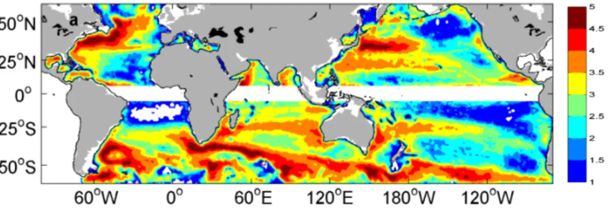
At the mesoscale, which here is referred to as horizontal scales larger than the first baroclinic Rossby radius of deformation of O(10–100 km), the hori- zontal flow is close to geostrophic balance. The geostrophic scaling is valid at small Rossby numbers (Ro<<1) and large Richardson numbers (Ri >>1) (Thomas et al., 2008). Most of the ocean’s kinetic energy at subinertial frequencies is contained in the geostrophic mesoscale eddy field (Ferrari and Wunsch, 2009). Figure 2 shows the surface eddy kinetic energy inferred from satellite sea level anomaly measurements. Enhanced eddy kinetic energy is found within the Southern Ocean along the Antarctic Circumpolar Current, in the western boundary current regions of the subtropical gyres and a weaker maximum shows up in eastern boundary upwelling systems e.g off California and Peru (Fig. 2). It is important to note that also subsurface eddies can be found in the ocean (e.g.McWilliams, 1985;D’Asaro, 1988;Molemaker et al., 2015). The sea level anomaly signal for such subsurface eddies is often very weak or not present. This makes it difficult to detect these eddies by satellite measurements. However, in the Peruvian upwelling regions these subsurface eddies make an important portion of the mesoscale eddy field (Colas et al., 2012) and can often only be seen by direct in-situ measurements as shown in section 5.
Figure 2: Global horizontal distribution of mean eddy kinetic energy in loga- rithmic form (of unit J/m2) based on altimeter data available by the AVISO Altimetry Operations Center. Figure is taken from (Xu et al., 2014)
Mesoscale eddies are generated via barotropic and/or baroclinic instabil- ity, where the former is a horizontal and the latter a vertical shear instability (Olbers et al., 2012). In the ocean interior baroclinic instability seems to be the dominant eddy kinetic energy source (e.g. von Storch et al., 2012). The Eady growth rate, given byωEady = 0.3f /√
Ri, is a good proxy for measuring
baroclinic instability (Eady, 1949;Olbers et al., 2012). Regions of enhanced Eady growth rates based on hydrographic data are indeed well correlated with high eddy kinetic energy (Chelton et al., 2007;Vollmer and Eden, 2013;
Thomsen et al., 2014).
In boundary current regions, strong lateral shear exists and barotropic instabilities and interactions with topography are also important for gener- ating mesoscale eddies (Gula et al., 2015). It is important to note that even if unforced mesoscale instabilities such as baroclinic and barotropic instabil- ity are mainly used to describe the generation of mesoscale eddies, several recent studies point out the importance of submesoscale instabilities and up- scale energy transfer for the generation of mesoscale features (Molemaker et al., 2015). This will be discussed in more detail later as it is of relevance for the eddy formation described in section 5. Mesoscale eddies further play an important role for the along-isopycnal tracer transport due to mesoscale stirring (section 2.7) and modulate biogeochemical processes (section 2.8).
2.3 Submesoscale frontal processes
Submesoscale frontal processes operate on lateral scales smaller than mesoscale eddies but are still influenced by rotation and stratification as they are char- acterized by Ro and Ri of O(1) (Thomas et al., 2008; Levy et al., 2012).
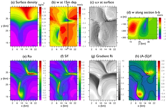
Figure 3a,b taken from (Thomas et al., 2008) shows the local Ro and Ri within a simulated flow field. Note the increase and decrease of the Ro and Ri, respectively in specific areas (e.g. at x = 14 - 22 km and y = 35 km). In submesoscale flows the relative vorticity ξ becomes comparable to the planetary vorticity f since Ro = U/(f L) = ξ/f = O(1). Different to mesoscale flows, submesoscale flows are only partly geostrophically balanced as advection of momentum plays a significant role.
The horizontal velocity or density gradients associated with submesoscale flows are found at a typical length scale L, which we want to derive here following (Thomas et al., 2008). This length scale is given by L = U/f as ξ ∼ U/L and Ro = U/(f L) = O(1). Assuming thermal wind balance U ∼ byh/f; the horizontal velocity scale U can be related to the lateral buoyancy gradient by and the mixed layer depth h, the vertical scale at which the velocity and lateral buoyancy gradients are dominant. It follows thatL=byh/f2. Using now the relationship between the lateral and vertical buoyancy gradients at an adjusted front N2 = b2y/f2 (Tandon and Garrett, 1994) the typical length scale can also be expressed in terms of stratification L = N h/f, where N is the depth averaged Brunt-V¨ais¨ala frequency and h a depth scale, which is often the mixed layer depth. Note the similarity to the first baroclinic Rossby radius of deformation describing mesoscale
motion, where h represents the full water depth. This results in a length scale L= 2.15km using typical values for the mixed layer depth of h = 15 m,N = 5×10⁻³s−1 and the Coriolis parameterf = 3.5×10⁻⁵ found during the summer season in the Peruvian upwelling regime (Koehn, 2014).
The inverse of the growth rate ωgrowth of baroclinic mixed layer insta- bilities given by 1/ωgrowth =√
Ri/f is often used as a typical time scale of submesoscale variability. This results in a typical time scale of O(1/f) since Ri = O(1) (Thomas et al., 2008). Both, the time and the length scale of submesoscale motion are influenced by the Coriolis parameter. This implies that submesoscale processes have longer timescales and larger lateral scales closer to the equator. Thus, a definition of submesoscale processes based on fixed length scales can be misleading because submesoscale flows are defined by their dynamics and the associated time and length scale vary with latitude and mixed layer properties.
Thomas et al.(2008) describe three different mechanisms that are respon- sible to generate submesoscale motions:
1) Unforced instabilities are one mechanism to generate submesoscale variability. If strong winds pass an oceanic frontal region, the enhanced wind-stress results in enhanced vertical mixing within the upper ocean and a deepening of the mixed layer. During the wind event the stratification in the upper ocean is reduced, but lateral density gradients can still be present.
Weak stratification, strong lateral density fronts and thus strong vertical shear are favorable conditions for submesoscale baroclinic instabilities as the Ri becomes small. Various studies have treated the unforced baroclinic insta- bility problem at low Ri (Stone, 1966, 1970, 1972;Haine and Marshall, 1998;
Boccaletti et al., 2007). More recent studies also highlight the importance of barotropic instabilities at submesoscale fronts which are driven by strongly laterally sheared flow (e.g. Gula et al., 2014).
2) Forced instabilities can grow under persistent atmospheric surface forc- ing. When wind blows in the direction of a frontal jet (i.e down-front), the as- sociated ageostrophic Ekman transport within the mixed layer results in the advection of denser water over lighter water, which leads to convective driven mixing. The associated redistribution of buoyancy can drive a geostrophy- restoring ageostrophic secondary circulation which further strengthens the front (Thomas and Lee, 2005a). Strong near surface loss of buoyancy as a result of air-sea heat flux also favors submesoscale variability as it decreases the Ri (Haine and Marshall, 1998). The role of forced instabilities along sub- mesoscale mixed layer fronts for the dissipation of kinetic energy is further discussed in section 2.6.
3) Frontogenesis, the intensification of a density front (Hoskins (1982), see more details in next subsection 2.4), is another mechanism to gener-
THOMAS ET AL.: SUBMESOSCALE PROCESSES AND DYNAMICS X - 3
Figure 1. A region in the model domain where spontaneous frontogenesis has set up large shear and relative vorticity, strain rates and a strong ageostrophic secondary circulation. (a) Surface density (kg m−3), (b) vertical velocity at 15 m depth (mm s−1), (c) surfaceu, vvelocities, (d) vertical section through the front atx= 16 km showing vertical velocity (red indicates upward, blue downward) and isopycnals (black), (e)Ro=ζ/f, (f) S/f, (g) gradient Ri, and (h) (A− |S|)/f with the zero contour shown as a dark black line. Light black contours indicate surface density.
motion, such as flows affected by buoyancy fluxes or fric- tion at boundaries. We will use the results from a numerical model to individually demonstrate the above submesoscale mechanisms. Even though the submesoscale conditions are localized in space and time, the mesoscale flow field is cru- cial in generating them. In the ocean, it is likely that more than one submesoscale mechanism, and mesoscale dynamics, act in tandem to produce a complex submesoscale structure within the fabric of the mesoscale flow field.
2.2. Frontogenesis
Consider the flow field generated by a geostrophically bal- anced front in the upper mixed layer of the ocean, overlying a pycnocline. As the front becomes unstable and meanders, the nonlinear interaction of the the lateral velocity shear and buoyancy gradient, locally intensify the across-front buoy- ancy gradient. Strong frontogenetic action pinches outcrop- ping isopycnals together, generating narrow regions in which the lateral shear and relative vorticity become very large, and the Ro and Ri become O(1). At these sites, the lat- eral strain rate S ≡ ((ux−vy)2 + (vx+uy)2)1/2 is also large, and strong ageostrophic overturning circulation gen- erates intense vertical velocities. In Fig. 1, we plot the density, horizontal and vertical velocities, strain rate, Ro, and Ri from a frontal region in a model simulation. The
deep mixed layer extending to 250m and allowed to evolve in an east-west periodic channel with solid southern and northern boundaries. Submesoscale frontogenesis is more easily seen when the mixed layer is deep, as the horizontal scale, which is dependent on H, is larger and more read- ily resolved in the numerical model. Here, the mixed layer is taken to be 250m deep in order to exaggerate frontoge- nesis. As the baroclinically unstable front meanders, the lateral buoyancy gradient is spontaneously, locally intensi- fied in certain regions, as in Fig. 1, generating submesoscale conditions at sites approximately 5 km in width. This mech- anism is ubiquitous to the upper ocean due to the presence of lateral buoyancy gradients and generates submesoscales when intensification can proceed without excessive frictional damping, or in a model with sufficient numerical resolution and minimal viscosity.
2.3. Unforced instabilities
The instabilities in the mixed layer regime where Ro= O(1) and and Ri = Ro−1/2 = O(1) are different from the geostrophic baroclinic mode in several respects. The ageostrophic baroclinic instability problem of a sheared ro- tating stratified flow in thermal wind balance with a con- stant horizontal buoyancy gradient was investigated using
Figure 3: Numerical simulation of a front undergoing frontogenesis. Two specific areas are of interest here (x1 = 14 − 22 km, y1 = 35 km and x2 = 8km, y2 = 17.5−25km), where cold filamentary intensification oc- curs. (a) Surface density, (b) vertical velocity, (c) surface u,v velocities, (d) vertical section of vertical velocity, (e) Rossby number, (f) Lateral strain rate Sstrain = ((∂u∂x − ∂v∂y)2+ (∂x∂v + ∂u∂y)2)1/2 divided by Coriolis parameter f, (g) gradient Ri and (h) stability criteria for unbalanced instability mode:
(A− |Sstrain |)/f. The criteria is met if the difference between the absolute vorticity (A =f+∂x∂v−∂u∂y) and the magnitude of the strain rate changes sign within the domain. For more details see (Molemaker et al., 2005; Thomas et al., 2008). Figure is taken from (Thomas et al., 2008)
ate submesoscale variability. When a geostrophically balanced mixed layer front becomes unstable and starts to meander, regions with horizontal con- vergence and divergence are formed leading to a large lateral strain rate Sstrain = ((∂u/∂x−∂v/∂y)2+ (∂v/∂x+∂u/∂y)2)1/2 and Ri and Ro of O(1).
An ageostrophic secondary circulation develops which is associated with en- hanced vertical velocities (Fig. 3b,d).
In the real ocean these different types of generation processes exist often simultaneously making it difficult to distinguish between them. In summary, submesoscale processes can be expected to play an important role if strong lateral density gradients resulting in strong vertical shear are accompanied
12
by weak stratification and strong atmospheric buoyancy loss.
2.4 Frontogenesis and cold filamentary intensification
Submesoscale variability covers a relatively broad range of scales including symmetric instabilities at some hundred meter scales to features such as filaments which have a typical length scale of several tens of kilometers but are only a few kilometres broad. Filaments play a key role in upwelling regimes as they transport productive coastal water offshore and downwards (Rossi et al., 2008, 2009; Nagai et al., 2015). Off the coast of Peru, cold filaments are uniquitous features seen in sea surface temperature fields and thus their dynamics will be described shortly.
example, a time-varying vorticity field with compact sup- port and finite circulation has a far-field velocity that is dominated by strain and can be locally Taylor-expanded around the frontal location, (x, y,z) = 0, as a dynamically inconsequential uniform velocity plus the deformation flow udplus higher-order spatial-polynomial components.
[7] Now consider the evolution of a localized flow pertur- bationu= (u,v,w), and its associated normalized pressure fluctuation8=p/r0and buoyancy fieldb=g(1r/r0) in the presence ofud.ris the density field, andr0is its mean value. To focus attention on the sharpeningxgradients, we assume for simplicity that the local flow perturbation is initially invariant iny; if so it will remain so for all time if
we neglect possible three-dimensional instabilities. We transform the two-dimensional Boussinesq equations from (x,z,t) to (X,Z=zeb,t), anticipating that frontogenesis and filamentary intensification will often sharpen gradients inz as well asx:D[u] fv+eb@X8=au;D[v] + fu=av;
D[w]b+eb@Z8= 0; &D[b] = 0;@Xu+@Zw= 0.D=
@t+u@X+ (w+aZ)@Zis the material derivative in (X,Z,t) where the advection by ud is implicit [McWilliams et al., 2009]. We decomposebinto its horizontal averagehbi(Z,t) and deviationb0(X,t), withhbi(z, 0) =N2z.
[8] We choose initial conditions with a surface-intensified b0(x, z, 0); a v(x, z, 0) in hydrostatic, geostrophic balance (f@Zv=@Xb0); and no ageostrophic secondary circulation (u=w= 0). Witha(0) = 0, this is a stationary state. We specify a(t) as an increasing function that asymptotes to a0 > 0 and induces frontogenesis and filamentary intensi- fication. (Its ramp-up over an interval of about 0.2a01
diminishes inertia-gravity wave excitation that would result from abrupt deformation.) Boundary conditions arew= 0 at the upper surface Z = 0 and vanishing perturbation velocity asZ! 1andX!±1. The problems of interest are frontogenesis with initialb0fro(x,z) =v0f‘0h01exp[z/h0] erf[x/‘0] and filamentary intensification with b0fil(x, z) = b0fro(x+d,z)b0fro(xd,z) whered= ±1.25‘0is chosen so that the filament has a single extremum inb0and approx- imately the same initialv and shear magnitudes as in the frontal initial condition (Figure 2). The sign ofddetermines the sign of the filamentary buoyancy perturbation; e.g., d> 0 is a positive (light, hot) anomaly. We choose parameter values relevant to submesoscale structures in subtropical oceans:v0= 0.1 ms1,h0= 33 m,‘0= 5 km,f= 104s1, N= 1.1102s1, anda0= 106. The associated buoyancy scale isb0=v0f‘0/h0= 1.5103m s2and temperature scale isT0=b0/Ag= 0.8 C (forA=@Tln[r] 2104C1).
[9] A common but severe dynamical approximation is quasigeostrophy (QG), where f@Zv = @X b0 exactly and ageostrophic advection is neglected inD. A further approx- imation is surface QG (SQG), where additionally the inte- rior QG potential vorticity is persistently zero (q=@Xv+ f@Zb0/N2= 0). The SQG solution to our posed problem is very simple for both frontogenesis and filamentary intensi- fication. The surface buoyancy perturbation is invariant in the transformed coordinates,b0(X, 0,t) =b0(x, 0, 0), hence its xscale shrinks in time as eb, and its gradientj@x b0j increases aseb. The interiorv(X,Z,t) andb0(X,Z,t) are also Figure 1. RADARSAT SAR image of the Santa Barbara
Channel at 1400 UT on January 8, 2003. The area is 100 km by 110 km. The image was provided by B. Holt, Jet Propulsion Laboratory, and processed at the Alaska Satellite Facility. (Copyright by the Canadian Space Agency (2003)).
Figure 2. (left) Sketches of surface frontogenesis and (right) cold filamentary intensification (d< 0).
L18602 MCWILLIAMS ET AL.: COLD FILAMENTARY INTENSIFICATION L18602
2 of 5
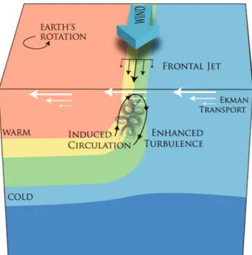
Figure 4: Sketches of surface frontogenesis (left) and cold filamentary in- tensification (right). On the right, a two-dimensional dense surface filament is undergoing frontogenesis in an external horizontal deformation flow (dot- ted–dash arrows) with uniform horizontal strain rate. Buoyancy contours (heavy solid lines) bulge up in the center, as labeled by ”light” and ”heavy”.
The approximately geostrophic longitudinal flow y (thin arrows) consists of a double jet. The ageostrophic secondary circulation (u, w) in the transverse plane (thick arrows) has central downwelling and peripheral upwelling, sur- face horizontal convergence, and subsurface horizontal divergence. Vortex stretching generates cyclonic vertical vorticity in the center and weaker an- ticyclonic vorticity on the edges. Figure is taken from (McWilliams et al., 2009, 2015) with modified text.
Filaments can be described as an elongated double frontal system which can be separated into warm and cold filaments. To better understand the dynamics involved in the development of cold filaments, it is helpful to re-
capitulate the mechanisms that are responsible for the strengthening of a density front by a confluent large scale flows, called frontogenesis.
Frontogenesis has been studied in the atmospheric context for decades (Hoskins, 1982) but also occurs in the upper ocean (Lapeyre et al., 2006;
Capet et al., 2008c). A sketch of this surface frontogenesis is shown in Figure 4a. Frontogenesis is caused by an external horizontal flow that deforms the flow field and yields strong horizontal density gradients. This deformation is responsible that the flow along the front has to accelerate. This accelera- tion drives an ageostrophic secondary circulation develops that restores the geostrophic balance of the front. Downwelling on the dense and upwelling on the light side of the front are typical characteristics of this secondary circulation (Fig. 4a). In the case of cold filamentary intensification (Fig.
4b), two fronts are aligned next to each other such that the center of this double front system is cold. Associated with these two fronts are two jets along each of the front resulting in large horizontal shear. Each of the two fronts contributes to the downwelling in the center of the front. This central downwelling is accompanied with a broader peripheral upwelling due to sur- face horizontal convergence and subsurface horizontal divergence. One open question is: Which factors ultimately limit the growth of frontogenesis when the straining deformation persists? This can be achieved by balanced insta- bilities as suggested by (McWilliams and Molemaker, 2011). Another more recent suggestion is that turbulence in the mixed layer and the associated momentum fluxes have to be taken into account when studying the arresting of frontogensis (Gula et al., 2014;McWilliams et al., 2015).
2.5 Internal waves and three-dimensional microscale turbulence
Surface waves found at the interface between the atmosphere and the ocean are a well known phenomenon for everyone looking at the ocean. However, also below the sea surface so-called internal waves are present, which lead to up- and downward motions in the water column. Internal waves propagate through the ocean interior and transport energy in the horizontal and vertical plane (Mueller and Briscoe, 2000).
Internal waves can be classified by their restoring forces, namely gravity or the Coriolis force. Gravity waves have a frequency close to the buoyancy frequency N and can only exist if a vertical density gradient is present.
If the Coriolis force is the main restoring force, internal waves are called near-inertial waves with a frequency near f. However, more common are so- called internal inertial-gravity waves, which are influenced both by gravity and the Coriolis force. The period of free internal gravity waves is limited
by the buoyancy period 2π/N, which has a typical range of 15 min in the upper ocean to several hours at greater depth, and by the inertial period 2π/f ≥12 h (Olbers et al., 2012).
Internal waves can have various wavelengths ranging from several thou- sand kilometers down to centimeters. Fluctuating wind stress, tides and flow-topography interactions can generate internal waves (Wunsch and Fer- rari, 2004). These propagate through the ocean where they interact with each other e.g. by resonant interaction (Mueller and Briscoe, 2000). Finally, small-scale internal waves can break, which results in turbulence and diapyc- nal mixing (Munk, 1966). Given that the internal waves provide an important energy source for the internal diapycnal mixing, they play an important role in the energy budget of the ocean circulation (Wunsch and Ferrari, 2004).
An important internal wave breaking mechanism is the so-called Kelvin- Helmholtz instability. It refers to the growth of small perturbations generated by the vertical shear of the horizontal velocity, which are not damped by the stratification. Mathematically the condition for Kelvin-Helmholtz instability to occur in a vertically sheared flow would be that Richardson numbers is below 1/4. This instability causes small-scale density overturns during the wave breaking which results in three-dimensional turbulence and diapycnal mixing (e.g. Smyth et al., 2001). This diapycnal mixing is important for tracer fluxes across isopycnals. Diapycnal mixing is crucial for the global ocean circulation as it results in a downward heat transport and allows the cold and dense water found in the deep ocean to upwell (Wunsch and Ferrari, 2004).
2.6 Submesoscale routes to dissipation
The ocean gains kinetic energy at large scales due to atmospheric and tidal forcing (Wunsch and Ferrari, 2004). Finally, this kinetic energy dissipates at molecular scales and is transferred into heat and potential energy (Wunsch and Ferrari, 2004). The processes that accomplish the transfer of energy are not well understood. One major question in understanding global ocean dynamics is: How is the kinetic energy gained by the large scale forcing transported towards the smaller scales where it can be dissipated?
The exchange of kinetic energy between different length scales is called an energy cascade. Mesoscale motion transfers energy to larger scales, a pro- cess known as an ’inverse cascade’ (Charney, 1971). Geostrophic turbulence therefore does not deliver an efficient pathway towards smaller scales (Mole- maker et al., 2010). However, breaking internal waves can transfer energy to small spatial scales into a regime of three-dimensional turbulence (Garrett and Munk, 1979). This regime of microscale turbulence is known to transfer
energy to even smaller scales called a ’forward cascade’ (Kolmogorov, 1941), where it is finally dissipated by molecular processes. Due to the inverse en- ergy cascade the mesoscale field plays an opposing role in energy transfer compared the internal waves and three-dimensional turbulent regime. How- ever, contrary to mesoscale motion, submesoscale frontal processes seem to be able to break the geostrophic balance resulting in a ’forward cascade’.
Recent studies show that submesoscale motion might deliver a pathway to extract energy from the geostrophic balanced state into the microscale tur- bulent regime (Molemaker et al., 2010; Brueggemann and Eden, 2015).
Molemaker et al.(2010) carried out two high-resolution numerical simula- tion to investigate the energy transfer between different scales. At first they studied an idealized Boussinesq flow, a flow system which allows ageostrophic motion, and found that a ’forward energy cascade’ directed towards small scale dissipation was established due to submesoscale frontal instabilities. As a second step the authors carried out a simulation with the same configura- tion but with a quasi-geostrophic model, which does not allow the advection by ageostrophic motion. This flow system was not able to establish a ’for- ward energy cascade’, which points to the importance of the unbalanced flow at frontal regions for this route to dissipation.
Submesoscale frontal instabilities occur along submesoscale fronts and are described in the following. Figure 5 illustrates the ongoing processes at a wind-forced symmetrically unstable front. At strong lateral density fronts, symmetric instability can occur due to the strong vertical shear of the geostrophic flow. When submesoscale fronts experience strong atmo- spheric wind forcing along the geostrophic frontal jet, the ageostrophic Ek- man flow destabilizes the water by bringing denser water over lighter water.
The stratification and the Ertel PV are reduced and the frontal structures are strengthened (Thomas and Lee, 2005a). Strong atmospheric cooling can also reduce the PV within the mixed layer. Symmetric instability takes its energy from the kinetic and potential energy of the front itself (Thomas and Taylor, 2010). Symmetric instability results in strong along-isopycnal shear which can drive secondary Kelvin-Helmholtz instabilities, which can lead to strong dissipation rates (Taylor and Ferrari, 2009). Symmetric instability can thus be seen as a mediator of dissipation. Thomas and Taylor (2010) carried out high-resolution numerical model simulations and demonstrated that winds blowing in the same direction as the frontal jet force symmetric instability.
These results are of particular importance as they present a new path- way to small scale dissipation via a forward energy cascade associated with submesoscale instabilities. These findings might help to solve the question of how the kinetic energy of the ocean gained by large scale forcing is trans-