1. Introduction
The Southern Ocean (south of 44°S, defined as in Lenton et al. 2013) plays a crucial role in the global car- bon cycle, acting as a major sink for modern anthropogenic CO2 and modulating, on longer time-scales, ocean-atmosphere CO2 partitioning through variations in the biological carbon pump, surface nutrient utilization, and deep-ocean ventilation (Gruber & Doney, 2019). Contemporary air-sea CO2 fluxes in the region reflect a combination of natural degassing to the atmosphere and anthropogenic CO2 uptake (Lenton
Abstract
The ocean coastal-shelf-slope ecosystem west of the Antarctic Peninsula (WAP) is a biologically productive region that could potentially act as a large sink of atmospheric carbon dioxide.The duration of the sea-ice season in the WAP shows large interannual variability. However, quantifying the mechanisms by which sea ice impacts biological productivity and surface dissolved inorganic carbon (DIC) remains a challenge due to the lack of data early in the phytoplankton growth season. In this study, we implemented a circulation, sea-ice, and biogeochemistry model (MITgcm-REcoM2) to study the effect of sea ice on phytoplankton blooms and surface DIC. Results were compared with satellite sea- ice and ocean color, and research ship surveys from the Palmer Long-Term Ecological Research (LTER) program. The simulations suggest that the annual sea-ice cycle has an important role in the seasonal DIC drawdown. In years of early sea-ice retreat, there is a longer growth season leading to larger seasonally integrated net primary production (NPP). Part of the biological uptake of DIC by phytoplankton, however, is counteracted by increased oceanic uptake of atmospheric CO2. Despite lower seasonal NPP, years of late sea-ice retreat show larger DIC drawdown, attributed to lower air-sea CO2 fluxes and increased dilution by sea-ice melt. The role of dissolved iron and iron limitation on WAP phytoplankton also remains a challenge due to the lack of data. The model results suggest sediments and glacial meltwater are the main sources in the coastal and shelf regions, with sediments being more influential in the northern coast.
Plain Language Summary
Some coastal ocean areas of Antarctica, like the West Antarctic Peninsula (WAP), have high biological productivity, which indicates they could absorb more atmospheric CO2. Studying these regions is hard since weather, clouds and sea ice make satellite and cruise data collection challenging. Using models is an alternative to fill in the gaps in the data. In this study, we used an ocean model that simulates circulation, sea ice, biological productivity, and the nutrient cycle in the WAP to study how much sea ice and biology influence the carbon cycle. We find that in years when the ice season is long there is a smaller flux of carbon between ocean and atmosphere, and more dilution of the surface waters by sea ice melt. Although the amount of inorganic carbon in the surface ocean is low by the end of the productive season, this does not reflect more CO2 being taken up or more biological productivity. In years of shorter sea ice season, in contrast, the ocean takes up more atmospheric CO2 and has a longer productive season. This is because the surface ocean is exposed for longer, so gas transfer happens more easily and there is more light available for photosynthesis.© 2021. The Authors.
This is an open access article under the terms of the Creative Commons Attribution-NonCommercial-NoDerivs License, which permits use and distribution in any medium, provided the original work is properly cited, the use is non-commercial and no modifications or adaptations are made.
Peninsula
C. Schultz1,2,3 , S. C. Doney1 , J. Hauck4 , M. T. Kavanaugh5, and O. Schofield6
1Department of Environmental Sciences, University of Virginia, Charlottesville, VA, USA, 2Department of Marine Chemistry and Geochemistry, Woods Hole Oceanographic Institution, Woods Hole, MA, USA, 3Department of Earth and Atmospheric Sciences, Massachusetts Institute of Technology, Cambridge, MA, USA, 4Marine Biogeoscience Division, Alfred-Wegener-Institut, Helmholtz-Zentrum für Polar und Meeresforschung, Bremerhaven, Germany,
5Ocean Ecology and Biogeochemistry, College of Earth, Ocean, and Atmospheric Sciences, Oregon State University, Corvallis, OR, USA, 6Department of Marine and Coastal Sciences, Center for Ocean Observing Leadership, School of Environmental and Biological Sciences, Rutgers University, New Brunswick, NJ, USA
Key Points:
• Longer growth season in years of early sea-ice retreat show higher seasonally integrated NPP, despite lower chlorophyll in January
• Sea ice is important for DIC drawdown as it influences the duration of phytoplankton bloom, air-sea CO2 fluxes, and dilution by meltwater
• In the WAP, sedimentary iron has a larger role in the northern coast and shelf, glacial meltwater likely the main source in the south
Supporting Information:
Supporting Information may be found in the online version of this article.
Correspondence to:
C. Schultz, cs3xm@virginia.edu
Citation:
Schultz, C., Doney, S. C., Hauck, J., Kavanaugh, M. T., & Schofield, O.
(2021). Modeling phytoplankton blooms and inorganic carbon responses to sea-ice variability in the West Antarctic Peninsula. Journal of Geophysical Research: Biogeosciences, 126, e2020JG006227. https://doi.
org/10.1029/2020JG006227 Received 18 DEC 2020 Accepted 18 MAR 2021
et al., 2013), with the southernmost latitudes representing only a small sink. However, large-scale estimates of air-sea CO2 fluxes do not adequately resolve the coastal regions of Antarctica, which can be highly pro- ductive biologically and act as strong sinks of anthropogenic carbon (Arrigo et al., 2008). Therefore, a better assessment of the role of the Southern Ocean in the global carbon cycle relies on improving the understand- ing of the air-sea fluxes and biological carbon cycling in the coastal areas of Antarctica and the fate of the excess carbon.
One of these productive coastal regions is the shelf-slope on the West Antarctic Peninsula (WAP), a sea- ice influenced marine ecosystem with relatively high primary production and net community production (NCP) during the summer season (Ducklow et al., 2013, 2018; Vernet et al., 2008), and air-sea CO2 fluxes indicate a strong sink of atmospheric carbon (Jones et al., 2017; Legge et al., 2015). Although the dissolved inorganic carbon (DIC) in the surface ocean is highly variable and controlled by a variety of physical and biological factors, such as respiration, freshwater inputs, brine rejection, and mixing with subsurface waters rich in DIC (Carrillo et al., 2004; Eveleth, Cassar, Doney, et al., 2017; Eveleth, Cassar, Sherrell, et al., 2017), primary production is estimated to have a large role in controlling DIC during the summer months (Legge et al., 2015).
Along the WAP, there are long-term trends in several physical variables. The period between the 1970s (when satellite measurements started) and the early 2000s exhibited a substantial shortening of the sea-ice season (Stammerjohn et al., 2008, 2012), and decades-long trends also showed an increase in the surface ocean temperature of the order of 1°C (Meredith & King, 2005), and melting of glaciers at an accelerating rate (Cook et al., 2005). Although a trend toward increasing atmospheric temperature was also observed, it leveled off and even reversed direction in some places since the late 1990s (Turner et al., 2016), impacting the cryosphere in the northern Antarctic Peninsula, where glacier recession has since slowed down (Oliva et al., 2017). Despite the long-term trends, the duration of the sea-ice season, as well as the intensity of the phytoplankton bloom and the surface carbon concentrations, show high interannual variability due to the influence of the Southern Annular Mode (SAM) and El Niño Southern Oscillation in the region (Ducklow et al., 2013; Hauri et al., 2015; Stammerjohn et al., 2008, 2012; Vernet et al., 2008). Positive phases of SAM and La Niña events lead to warmer conditions and less sea ice along the WAP, with colder years and a longer sea-ice season observed in negative SAM and El Niño years. These modes of climate variability also reinforce each other in this region, with years of associated + SAM/La Niña (-SAM/El Niño) showing even warmer (colder) conditions (Stammerjohn et al., 2008).
Understanding the mechanisms behind the variations in primary productivity and DIC in the WAP is im- portant not only to quantify its present contribution to the global carbon cycle, but also to predict the chang- es that will occur under increased glacial meltwater input and warmer conditions. Field sampling of the re- gion, however, is limited by the presence of sea ice and harsh weather during much of the year. The Palmer LTER (Long Term Ecological Research) project (Ducklow et al., 2012, 2013) provides a valuable data set that includes physical, biological, and chemical variables from cruises performed during the months of January and February each year since 1993, but the data is still limited in time to mid-summer conditions. While satellite chlorophyll data helps to fill in the gaps in assessing the strength of the phytoplankton blooms, the data is biased toward ice-free and noncloudy areas, making it hard to assess the timing of bloom initiation.
Although primary production in the WAP is patchy and can vary by an order of magnitude from year to year (Vernet et al., 2008), some characteristics are observed consistently. Phytoplankton blooms follow the retreat of sea ice, peaking first in the northern and offshore areas, and there is a consistent onshore-offshore gradient, with coastal and shelf waters being up to eight times more productive than offshore regions (Li et al., 2016). The blooms are dominated by diatoms with secondary contributions from cryptophytes (Brown et al., 2019; Schofield et al., 2017), and the main mechanism controlling its progression is thought to be light limitation. Macronutrients are abundant (Kim et al., 2016) and micronutrient iron limitation is not observed in the coastal areas (Carvalho et al., 2016), although it is expected in the offshore regions (Annett et al., 2017; Arrigo et al., 2008; Li et al., 2016). Summer DIC measurements show lower concentrations than would be expected from dilution due to meltwater and glacial input, indicating that they are influenced by biological net community production (Hauri et al., 2015; Legge et al., 2015).
Given the high interannual variability of the blooms and the patchiness observed during individual years, however, the importance of different processes in controlling the timing and intensity of the bloom, as well as long-term trends, remain unknown. The long-term trends in chlorophyll based on satellite ocean color observations were estimated to be negative in the northern part of the grid and positive in the southern part (Montes-Hugo et al., 2009), related to sea ice decrease, winds, and changes in mixed layer depth (MLD).
With less sea ice in the northern part of the WAP, where more light is available throughout the year, the region is more exposed to wind mixing, which deepens the MLD and lowers photosynthetically available radiation (PAR). In the southern WAP, areas that were previously completely covered by sea ice had an in- crease in PAR and higher productivity.
Kim et al. (2018), however, found a trend of increase in chlorophyll values for near-shore time-series sites at Palmer Station and Potter Cove (in the northern part of the WAP), and a decrease in Rothera Station, in the southern region, driven by a sea-ice rebound that started in 2009. A trend toward lower biomass at Rothera Station was also observed by Rozema et al. (2017), with summer biomass thought to be lower following winters with low sea ice concentration that lead to less stable water column (Rozema et al., 2017; Venables et al., 2013).
While macronutrients are known to be abundant in the WAP, the concentrations of dissolved iron (dFe) as well as their sources are not well constrained. It is unknown, therefore, the role dFe plays in controlling the intensity and patchiness of the bloom. This is due to the fact that collecting in situ seawater dFe data is a challenging process, and this micronutrient is undersampled in the WAP compared to macronutrients and biological data. Studies available, performed with relatively small data sets, reach conflicting conclusions regarding the source of dFe and how it limits primary production in different places and seasons.
During a cruise performed in the spring, Arrigo et al. (2017) observed a correlation between dFe and re- duced sea ice, indicating that ice melt could be a source of iron. One caveat, however, is that freshwater lenses were not linked to the higher dFe concentrations. Glacial freshwater appears to be a dominant source of dFe during the summer in parts of the shelf (Annett et al., 2017) and in Ryder Bay, a coastal area toward the south of the WAP (Annett et al., 2015; Bown et al., 2018). In Ryder Bay, dFe was also replenished over annual periods via vertical mixing with dFe-rich subsurface waters. Toward the north of the WAP near Palmer Station, Sherrell et al. (2018) found that high dFe was linked to sediment sources in coastal areas, which were transported to the shelf and fueled production near Palmer Deep Canyon. Sherrell et al. (2018) also found no connection between high dFe and glacial inputs. The studies available to date, therefore, indicate that there are temporal and spatial variations in which the source of dFe is dominant in the WAP.
It has been established that lower DIC concentrations are associated with higher primary production in the late summer (Hauri et al., 2015; Legge et al., 2017), but it is not clear how these two variables co-vary throughout the season. Although normalizing DIC to salinity helps to estimate the biological effect of draw- down by roughly correcting for dilution, variations in MLD change the expected end-member concentra- tions for DIC and salinity throughout the season through mixing with DIC-rich and more saline sub-surface waters.
In this study, we use a coupled ocean circulation, sea-ice, and biogeochemistry model to fill some of the gaps in the understanding of the mechanisms controlling phytoplankton bloom and its impact on the surface DIC concentration in the WAP. We compare the model results to cruise data from the Palmer LTER project and to satellite data to validate the model results, and discuss some of the limitations from each method due to the spatial and temporal coverage.
2. Methods
2.1. Model Description
The ocean circulation and sea-ice model used for this study (similar to the CTRL simulation described in Schultz et al. [2020]) is a regional domain version of the Massachusetts Institute of Technology General Circulation Model (MITgcm), with a hydrostatic setup that includes embedded sea-ice and ice-shelf mod- ules. The grid used, shown in Figure 1, covers the region extending from 74.7°S, 95°W in the southwest to 55°S, 55.6°W in the northeast, with a horizontal resolution of 0.2° of longitude and ranging from 0.0538° to
0.1147° latitude, corresponding to cells ranging from 5.98 km in the south of the domain to 12.75 km in the north. On the vertical, it uses z-level (fixed depth) with 50 layers spaced every 10 m for the first 120 m. The atmospheric forcings were obtained from the ERA-Interim reanalysis (Dee et al., 2011) with a horizontal resolution of 1.5° in latitude and longitude and a 6-h interval. Freshwater runoff representing melt of land- based ice and iceberg calving and melting is provided with monthly climatological estimates, using the values estimated by Van Wessem et al. (2016) distributed uniformly along the coast and linearly decreasing from land out to 100 km. Although the ice shelves include a freshwater component, they are not considered a source of dFe. The grid used is shown in Figure 1, and more details on the implementation of the ocean physical circulation and sea-ice models are described in Regan et al. (2018) and Schultz et al. (2020).
The biogeochemical model used is the Regulated Ecosystem Model version 2 (REcoM2), described in Hauck et al. (2013, 2016). REcoM2 has 21 components, including two phytoplankton groups (diatoms and small phytoplankton), one zooplankton group, and organic and inorganic forms of the main nutrients (iron, ni- trogen, silica, and carbon). Although not added as a group, bacteria functionality is represented via remin- eralization. Emphasis is given to phytoplankton physiology, with variable cellular stoichiometry and phys- iological rates that depend on the intracellular ratios of nitrogen to carbon (N:C), chlorophyll to carbon (Chl:C), and silica to carbon (Si:C). Phytoplankton chlorophyll is calculated as a function of irradiance and nitrogen assimilation, degraded at a constant rate, and lost by aggregation and grazing. A parameterization to include nonlinearities in PAR due to the influence of partial sea-ice coverage was added following Long et al. (2015).
The sources of DIC are respiration, remineralization of detritus, and dissolution of calcium carbonate, while sinks are fixation by primary production and formation of calcium carbonate. Alkalinity increases by nitrogen assimilation and dissolution of calcium carbonate and decreases by remineralization and calcifica- tion. Air-sea CO2 fluxes are calculated with code based on the Ocean Carbon-Cycle Model Intercomparison Project (OCMIP), which uses a quadratic relationship with wind based on Wanninkhof (1992). The surface CO2 concentration is calculated at every time-step using simulated DIC, alkalinity, temperature, and salini- ty, and the gas exchange is treated as a boundary condition for DIC.
Figure 1. (a) Map of model bathymetry for the full Southern Ocean sector for the West Antarctic Peninsula (WAP) with the region of Palmer-LTER cruises marked in the blue rectangle and Palmer Station marked in the red circle, and (b) a larger scale map of coastal-shelf-slope (WAP) overlain with locations of the Palmer-LTER cruise sampling stations. Blue dots represent the coastal points sampled, yellow dots represent the shelf points sampled, and red dots represent the slope points sampled. The transect lines in the southern region are lines 200 (southernmost) and 300, and the transect lines in the northern region are 400, 500, and 600 (northernmost). Sub-regions analyzed are named northern coastal (n_cs), northern shelf (n_sh), northern slope (n_sl), southern coastal (s_cs), southern shelf (s_sh), and southern slope (s_sl).
Total dissolved iron (dFe) is assumed to be the sum of inorganic bound and organic complexed (FeL, where L is a ligand) iron. These two forms are in equilibrium according to:
FeL
K Fe L
(1)FeL
where KFeL is the equilibrium constant and Feʹ is the concentration of free iron. Iron is added to the model via atmospheric deposition and as glacial input, and internal model sources include respiration, remineral- ization (including diagenetic sediment source), and heterotrophic excretion, while sinks are represented by scavenging (proportional to detritus concentration) and photosynthesis.
2.2. Initial and Boundary Conditions for REcoM2
Initial and boundary conditions for dissolved inorganic nitrogen and silicate (DIN and DSi) were obtained from the World Ocean Atlas 2013, version 2 (WOA13v2, Garcia et al., 2014). Monthly climatologies were used from the surface to 500 m, with annual climatology applied below this depth. DIC and alkalinity were obtained from the 1° resolution gridded Global Ocean Data Analysis Project version 2 (GLODAPv2, Key et al., 2015), with DIC representing contemporary concentrations centered in 2002 (Lauvseth et al., 2016).
Atmospheric CO2 remains constant, at 380 ppm. Since dFe data is scarce, the initial and boundary condi- tions for this nutrient were obtained from a version of MITgcm-REcoM2 configured globally without the Arctic region, described in Hauck et al. (2016).
Atmospheric deposition and glacial sources of dFe are also represented in the model. Dust deposition is derived from the Model of Atmospheric Transport and Chemistry (MATCH), detailed in (Luo et al., 2008).
Glacial inputs could be a significant source of iron to the region, but there is a lack of data on glacial concen- trations of this micronutrient. Annett et al. (2017) estimated meteoric concentrations of dFe of 102 nmol/
kg based on the difference of meteoric water (obtained from oxygen isotopes) and seawater dFe measure- ments performed between 2011 and 2012. The high concentrations are due to a source mechanism involv- ing dFe-enriching subglacial processes and glacial meltwater streams. To avoid modifying the code, and taking advantage of the fact that input of freshwater is done at the surface, the glacial input of dFe was calculated to scale to the surface runoff at a concentration of 100 nmol/kg, but added to the same file as the atmospheric deposition.
The largest atmospheric deposition value in the grid is in July, with values reaching 0.03 µmol/m2d in the northernmost latitudes of the model grid. Since glacial sources are much larger than atmospheric deposi- tion and do not depend on SIC, we opted not to scale the deposition by sea ice concentration, with the full amount of dFe being deposited even in the presence of sea ice. Although the glacial dFe sources include seasonal variation, one caveat of this approach is that neither glacial inputs of freshwater or dFe include interannual variability. Other caveats are that there is no latitudinal variability in the glacial dFe sources and that no dFe is present in ice shelf basal meltwater, which is expected to have a larger influence in the southern region and in Marguerite Bay.
2.3. Experiment Description
The historical physical-biogeochemical simulation builds upon an existing ocean-sea ice physical hindcast simulation with the WAP MITgcm (Schultz et al., 2020). The model physics is forced by atmospheric rea- nalysis at the surface, seasonally varying glacial freshwater input from the Peninsula, and simulated ocean physics and sea-ice climatologies at the lateral boundaries from a large-scale, low-resolution circumpolar MITgcm simulation (Holland et al., 2014). Schultz et al. (2020) present a detailed assessment of the physical model behavior and skill in terms of the geographic patterns, of seasonal cycle, and of interannual variabil- ity of the ocean MLD, sea-ice concentration (SIC), and freshwater dynamics for the WAP coastal-shelf-slope region.
Overall the model (similar to simulation CTRL in Schultz et al. [2020]) performs well in capturing region- al sea-ice variations from satellite observations, reflecting local thermodynamics of sea-ice formation and melt and wind-driven sea-ice advection and convergence. The model also does a credible job in simulating
summertime MLD patterns found in the Palmer LTER CTD data set, though the simulated MLDs tend to be biased somewhat shallow compared to the field data. Biases ranged from 8.9 m shallower in the southern slope region to 23.2 m shallower in the southern coastal region when comparing the simulated average January–February MLD to the Palmer-LTER cruise data. MLD reflects the complex interactions of wind-driven mixing (influenced by sea ice, which shields the surface ocean), seasonal heating and cooling, brine rejection and sea-ice melt, freshwater sources like glacial runoff and icebergs, and lateral circulation.
The MLD biases were improved to some extent with better model treatments of Langmuir circulation and air-sea ice drag.
The physical-biogeochemical model was integrated for 31 years, from 1984 until 2014, in a similar fashion to the physics-only simulation. The first 7 years of integration (1984–1990) are considered spin-up and the results are analyzed from 1993 (first year of the summer Palmer-LTER cruises) onward. Diagnostic outputs for simulated physics, nutrients, chlorophyll, net primary production (NPP), DIC, and air-sea CO2 fluxes were saved every 5 days.
Two passive tracer experiments were conducted to assess whether sediment diagenetic sources of dFe to the water column could impact the concentration in the mixed layer. For these experiments, the climatological monthly mean fluxes of dFe from sediment to the water column were calculated, and it was determined that in the coastal and shelf waters, there is a seasonal difference, with more iron being released late summer and less in the spring (Figure S1). This cycle reflects the phytoplankton bloom with an added lag, given it takes time for organic matter to reach the bottom and be remineralized. The first passive tracer experiment used a tracer that accounted for the total climatological amount of iron being released from the sea floor during the month of February. At every grid point, a diagenetic dFe concentration anomaly (μmol/m3) was computed for the bottom layer grid cell assuming that all of sediment Fe flux (μmol/m3/d) for the entire month of February accumulated in the bottom layer. The tracer was released at the bottom layer on the first day of February 1991, after the spin-up, and the concentration of the passive tracer was tracked during the next year. A second experiment used the same approach but using the diagenetic concentration of dFe of July, and released the tracer on the first day of July 1991.
2.4. Calculation of DIC-Derived Net Community Production
The metabolic balance of the whole ecosystem is determined by NCP, which also governs the potential for biomass accumulation and carbon storage in the system. NCP is used, in this study, to assess the influence of primary production in the DIC drawdown throughout the summer in the WAP. Since NCP is not a diag- nostic variable of the model, it was calculated from the DIC drawdown between September and January.
September was chosen as the start of the season since it is the earliest the phytoplankton bloom can start.
For each station, the total DIC inventory for each month was calculated as the vertically integrated DIC from the September MLD to the surface. Since the mixed layer shoals during the period considered, using the September MLD guarantees that vertical mixing effects will not influence the inventory calculations performed.
The total DIC drawdown was then corrected for air-sea CO2 fluxes and for dilution by sea-ice melt. The air-sea CO2 flux is a diagnostic of the model, and the dilution by sea-ice melt was calculated using a salinity mixing curve. The hypothetical DIC inventory (integrated from the September MLD to the surface) at the end of the season (January) in the case where melt was the only process affecting it would be:
Sep 0 Sep
Sep Sep Jan
_ dil MLD
MLD DIC
Int DIC
MLD melt ‐
(2)
where MLDSep is the September MLD, 0MLDDICSep is the vertically integrated DIC in September (from bot- tom of MLD to the surface), and meltSep Jan‐ is the total sea-ice melt during the season (September–January), given in meters. For this calculation, it is assumed that sea-ice had a DIC concentration of zero. The DIC drawdown due to sea-ice melt, then, would be:
0
_ Sep _ dil
Int DIC MLD DIC Int DIC
(3)
Although meteoric sources of freshwater (atmospheric and glacial runoff) are present in the model, sea ice melt represents a larger freshwater input and is responsible for most of the variability observed in the fresh- water content (Figure 7 in Schultz et al., 2020). The influence of glacial runoff also decreases significantly away from the coastal region. Dilution by glacial sources, therefore, was not calculated. Once corrected for atmospheric fluxes and melt, the remaining DIC drawdown is assumed to be due to biological activity and therefore can be equated to NCP. The seasonally integrated (September–January) NCP, therefore is calcu- lated as:
_ 2
SONDJ SONDJ CO
NCP DIC Int DIC F
(4) where DICSONDJ is the total DIC drawdown and FCO2 is the air-sea CO2 flux. The DIC-calculated NCP is then compared to NPP, which is a diagnostic variable from the model. These calculations were done for each station and averaged for each sub-region. The calculations were also performed for the period between September and March, and corrected NCP and total NPP are shown in the supplements (Figure S7) for ref- erence. Although the patterns observed are similar, the calculated NCP is less reliable given the mixed layer can deepen between January and March.
2.5. Data Used for Skill Assessment
The Palmer LTER started in 1991 and has collected physical, biological, and chemical data along the WAP since then (http://pal.lternet.edu/data). The data include semiweekly water-column sampling near Palmer Station on the southern end of Anvers Island from October through March and an oceanographic cruise in January–February each year since 1993 (Ducklow et al., 2013). The data collected during the cruises include CTD (conductivity, temperature, and depth) casts, chlorophyll-a concentration, zooplankton abun- dance, DIC, alkalinity, and nutrients. While Palmer Station has higher temporal resolution on the data, the station data is more affected by islands, near-shore bathymetry, and synoptic-scale phenomena that are not captured by the model. The cruise sampling grid is too coarse to resolve mesoscale features given the short Rossby radius on the shelf, a conclusion that is supported by studies using underway data from Palmer LTER cruises (Eveleth, Cassar, Doney, et al., 2017; Eveleth, Cassar, Sherrell, et al., 2017). Individual sam- pling stations can also be affected by phenomena such as the passage of icebergs, which will not be captured by the model. Clustering the cruise stations in sub-regions and calculating the climatological values and their anomalies makes it more likely that the data will represent the seasonal variations at a larger spatial scale; and could therefore be more accurately compared to the model data.
This study uses data from lines 200 to 600 of the Palmer LTER grid, spanning 500 km along the coast and 250 km across the shelf. As shown in Figure 1b, the across-shelf transects are separated by 100 km, with stations 20 km apart in each transect. All the data are available on the project web page (http://pal.lter.edu/
data/). Not all stations are sampled for all variables measured by the project each year, and each measure- ment does not necessarily reflect the mean state of the water column during the summer. To decrease the influence of short-term and small-scale processes, the cruise data were divided into north (lines 400–600) and south (lines 200 and 300) regions, and into coastal, shelf, and slope regions, based on bathymetry.
Six different regions are therefore analyzed: northern coastal (n_cs), northern shelf (n_sh), northern slope (n_sl), southern coastal (s_cs), southern shelf (s_sh), and southern slope (s_sl).
Level 2 remote sensing reflectances (Rrs) from Aqua-MODIS (v. 2018) and SeaWiFs (v.2018) spanning 1997–
2018 were downloaded from NASA Goddard and binned to a common 10 km grid (Kavanaugh et al., 2015).
Chlorophyll-a concentration was calculated per image using an algorithm tuned specifically for the WAP (Dierssen & Smith, 2000). While this algorithm was tested during SeaWiFs era, the superior skill has been confirmed with vicarious comparisons using 1 km Aqua-MODIS data and modern in situ chlorophyll-a from recent Palmer LTER station and cruise data (Kavanaugh et al., 2015). As the WAP can experience mul- tiple overflights per day, a daily composite was calculated over the grid, from which an 8-day and monthly averages were calculated using geometric means. SeaWiFs and MODIS time series were merged using the method of Kavanaugh et al. (2018), which applies a per-pixel seasonal correction to SeaWiFs data.
Sea-ice satellite images are obtained from GSFC (Goddard Space Flight Center) Bootstrap algorithm (Com- iso, 2017). Climatological and monthly mean SIC are calculated from binned 8-day means with horizontal
resolution of 0.2° in latitude and longitude. Onset time of sea-ice advance is chosen to be the day in which the average SIC of all the stations in each Palmer LTER sub-region reaches at least 0.15 (15% of the area covered by sea ice) for 5 days in a row. Sea-ice retreat is assumed to be the last day in which SIC is greater than 0.15 for the ice season. Further details are provided in Stammerjohn et al. (2008, 2012).
3. Results
3.1. Iron Sources in the Model
Given the low temporal and spatial coverage of available in situ dFe data, questions regarding the mecha- nisms that supply this micronutrient to different regions in the WAP, as well as how limiting iron is to pri- mary production, still persist. While Arrigo et al. (2017) argues that sea ice could be a major source during early spring, Annett et al. (2017) found that glacial meltwater was associated with higher dFe and Sherrell et al. (2018) found that dFe in coastal areas was supplied by sediment sources near Palmer Deep canyon.
In the model, atmospheric deposition of iron is negligible, and the sources of dFe to the mixed layer are glacial input, entrainment from below the mixed layer, or transport from other locations, including from the bottom layer which is enriched via sediment diagenetic processes. The glacial source of dFe is prescribed;
climatological estimates of freshwater runoff were uniformly distributed along the coast and decreasing linearly in volume from the shore out to 100 km from the coast, and a concentration of 100 nM of dFe was added to this runoff. The entrainment from below the mixed layer was calculated from the monthly clima- tology using the equation:
ent dMLD
F dFe
(5)dt
where dMLD/dt is the deepening of the MLD from month to month and dFe is the dFe concentration difference between the mixed layer and the layer below. The simulation (computes diapycnal diffusivities and vertical mixing using the K-Profile Parameterization [KPP; Large et al., 1994]) with a parameterization for Langmuir circulation added (Schultz et al., 2020). Mixing due to shear instability is calculated as a function of Richardson number, while internal wave activity is assumed constant. Equation 5 is only valid for periods of deepening mixed layer, since the subsurface dFe concentrations are consistently higher than the concentrations in the mixed layer. The fluxes during shoaling periods were set to zero, since no dFe was added to the mixed layer. Estimating the influence of sediment dFe at a certain location is more difficult given the role of circulation and transformation processes while iron makes its way from the sediment to the mixed layer. Using the concentration of the passive tracer experiments described in the Methods (Section 2.3) can give us an idea of where this source could be significant, but quantifying how much dFe comes from the sediment is not the goal of this experiment given that, unlike a passive tracer, iron could be consumed and transformed along the way from the sediment to the sub-regions of interest.
Figure 2 shows the flux of glacial and entrainment sources to the mixed layer (in orange, red), and the concentration of passive tracers in the ML during the year following their release (in black). Diagenetic dFe is a major source only in the northern coastal region, having a smaller impact in the southern coast and northern shelf, and no impact in the southern shelf and slope regions. Glacial sources, as expected from the design of the forcing files, have diminishing importance from the coast to the slope areas. Entrainment from below the mixed layer is a source of iron from late summer to early spring in the shelf and slope, but this mechanism of iron enrichment is halted from August through February while the mixed layer shoals.
This analysis shows that there is an (expected) difference in terms of iron supply between coastal, shelf, and slope areas, but also that there is a difference between the northern and southern regions, stronger in the coastal region. The model results indicate that in the northern coastal area, which is shallower and more influenced by circulation around the islands, sedimentary processes are a major source of dFe, while in the south glacial input is the dominant source of dFe. If shelf basal melt was included in the model, we suspect the importance of glacial melt in the south would be even larger. This difference validates the hypothesis suggested in Sherrell et al. (2018) that the discrepancies found between their study and the study of Annett et al. (2017) could be due to different sources having different impacts throughout the WAP. While Annett
et al. (2017) found the highest correlations between meteoric water and dFe in the southern part of the grid, the study of Sherrell et al. (2018) was aimed at understanding Palmer Deep, located near-shore and closest to line 600 (north).
While we suspect that the subsurface concentration of dFe in the model is higher offshore than would be observed due to the values used for the initial and boundary conditions, there is no data to validate this assumption. Other limitations concern significant uncertainties about the transformation and scavenging rates for dFe along the WAP, the absence in the model of dFe in sea ice and basal ice shelf melt, and the lack of temporal and spatial variability in the glacial dFe source used. It is possible, however, that the higher iron concentrations found in regions of low sea ice in the slope region, as found in Arrigo et al. (2008), could be at least partially explained by the fact that low sea ice concentration promotes mixing of surface waters with iron-rich subsurface waters by enhancing wind action. While surface mixing does not preclude the influ- ence of sea ice as a possible source of dFe, this mechanism would explain the absence of freshwater lenses in the low sea ice areas observed by Arrigo et al. (2008).
3.2. Model Skill in Reproducing Phytoplankton Bloom Climatology
To assess the model skill in reproducing the observed bloom climatology, we compared the monthly mean surface chlorophyll concentrations and SIC from the model with the monthly mean satellite data, shown for the period between November and February in Figure 3. Similar to observations, the simulated progression of the bloom follows the retreat of sea ice from offshore to onshore and from north to south. In parts of the grid, particularly the southern shelf and slope, however, the start of the bloom happens later in the model due to a delay in the modeled sea-ice retreat in this region, which leads to lower PAR at the beginning of the season.
The model also simulates the onshore-offshore gradient in surface chlorophyll seen in the observations, with higher concentration in the coastal and shelf areas. The simulated chlorophyll, however, has higher values in the coast and shelf regions in December and in the offshore areas throughout the season. It is thought that primary production offshore is limited by iron (Garibotti et al., 2005), which is not the case in the model as shown in the seasonal progression of the limitation terms, shown in Figure S2. Given the lack of iron data in the region, particularly farther from the coast, the understanding of the iron dynamics is limited and it is not possible to derive initial and boundary conditions from observations. Therefore, it Figure 2. MITgcm-REcoM simulated glacial fluxes of dFe (orange), dFe entrainment from below the ML (red) in nmol/m3d (y-axis scale on the left of plot).
Dotted lines in black and gray represent the concentration of passive tracers (January and July, respectively) released at the bottom in the mixed layer of each sub-region in the year following their release (y-axis scale on the right of plot). Notice the different y-axis scales for coastal regions compared to shelf and slope regions.
is possible that the model derived subsurface dFe, which reaches concentrations of 0.75 µmol/m3 in all sub-regions, is too high; leading to the higher chlorophyll values. The model also shows a sharper decrease in chlorophyll from January to February compared to the satellite data.
For each Palmer LTER survey cruise station, the data from the nearest model and satellite grid points were extracted, and the evolution of the surface chlorophyll concentrations and SIC are shown in Figure 4 along with the Palmer LTER surface chlorophyll data, assumed to be the January mean. Although the Palmer LTER data only has one data point per station each year, making it hard to assess whether each data point is representative of the regional values for that year, the climatological mean (calculated as the geometric mean of all the stations for each sub-region between 1993 and 2014) is comparable to the satellite climatol- ogy. The Palmer LTER and satellite data are similar in the northern region, while in the south, the satellite shows slightly higher surface chlorophyll concentrations.
Although the simulated bloom starts later than observed in the satellite data, the timing of the peak of the bloom coincides with the observations in much of the grid, with the exception of the southern slope. The model chlorophyll values also show the lowest summer values in February, with slightly increased concen- trations in March. Given that PAR availability in March is lower than in February, this can be attributed to iron limitation. The iron limitation terms are lowest in January, indicating high consumption during this month and leading to lower chlorophyll concentrations in early February before iron is replenished by deepening of the mixed layer.
3.3. Interannual Variability of the Phytoplankton Bloom
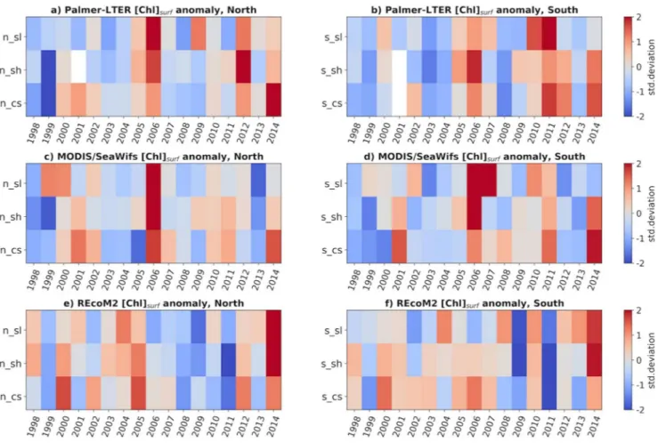
To analyze the interannual variability of the phytoplankton bloom, the anomalies (relative to the climatol- ogy) of surface chlorophyll concentration were calculated for each sub-region and for each data set (Fig- ure 5). For this comparison, the January monthly means were used for the satellite and model data, and the reference period from which the anomaly was calculated was from 1998, when satellite measurements Figure 3. MITgcm-REcoM2 (top) and MODIS/SeaWifs (bottom) climatological surface chlorophyll concentration for November, December, January, and February (left to right). Black dashed line shows SIC equal 0.5, and black full lines show SIC of 0.9.
Figure 4. MITgcm-REcoM2 (light blue dashed line) and GSFC (gray dashed line) climatological monthly sea ice concentration; MITgcm-REcoM2 (green) and MODIS/SeaWifs (black) log-transformed climatological monthly surface chlorophyll concentration; Palmer-LTER log10-transformed climatological surface chlorophyll concentration (red dot, plotted as January mean), during July–June, for regions n_cs (a), s_cs (b), n_sh (c), s_sh (d), n_sl (e), and s_sl (f). Vertical lines represent standard deviation.
Figure 5. Surface chlorophyll concentration anomalies, relative to the cruise climatology for Palmer-LTER data (a and b), and relative to January climatology for MODIS/SeaWifs (c and d) and MITgcm-REcoM2 (e and f); for northern region (a, c, and e) and southern region (b, d, and f).
started, until 2014. The figure shows discrepancies among the data sets, which could be attributed to the limited data collection and the patchiness of the bloom.
Retreat of sea-ice can be early during some sub-regions and late in others (Figure S3), depending on tem- perature and wind patterns throughout the season. Sea-ice ridging in the coastal areas can happen as sea- ice gets pushed from the slope and shelf areas. In the years in which sea-ice retreat happened consistently early in all sub-regions, such as 1999 and 2009, surface chlorophyll anomalies were mostly negative or close to neutral in all data sets, while years of consistent late sea-ice retreat like 2005 and 2014 showed mostly positive or low negative anomalies. The exception for this pattern is coastal chlorophyll anomalies from the MODIS/SeaWifs data set in 2005, which showed negative anomalies. In 2005, however, satellite images were scarce in the coastal region (1 in the northern coast and 4 in the southern coast), and it is possible that the satellite data missed the peak of the bloom during this season.
It is also worth noting that one of the limitations of the model is that it does not have interannual variability in the glacial discharge. This could be the cause of the lower chlorophyll concentrations simulated in some of the years in which satellite and cruise data show large blooms, such as 2006 and 2011. The year 2011 is one of the only years for which dFe data is available, and Annett et al. (2017) found that this year had much larger dFe and glacial meltwater concentrations compared to 2010 and 2012, particularly in the southern region, leading to an anomalously productive season. This was also a year of anomalously early sea-ice re- treat, which would otherwise lead to an early bloom and deeper MLD in January, usually indicative of lower chlorophyll concentrations during this month.
Although there are marked differences between the MODIS/SeaWifs and Palmer LTER data, the corre- lations in time (using the January means for satellite and model data, and cruise data) calculated for the surface chlorophyll for each sub-region range from 0.52 in the northern slope to 0.73 in the southern shelf and are larger than the correlations between these data sets and the model data (Table S1). The only sig- nificant correlation (at the 95% confidence level) for the simulated data was with the Palmer-LTER data in the northern coast (0.54). In years in which all sub-regions showed anomalous early or late sea-ice retreat (Figure S3), however, there was an agreement between the data sets on whether this was a high or low chlo- rophyll year in January. The seasons of 1998–1999 and 2008–2009 were chosen to represent years of early sea-ice retreat, with negative chlorophyll anomalies in all data sets; and 2004–2005 and 2013–2014 were chosen to represent years of late sea-ice retreat, with positive chlorophyll anomalies. Although 2011 also showed early sea-ice retreat, it was not considered in analyses in the next sections due to the anomalously high dFe observed, which would mean it does not necessarily represent the mechanisms that took place during the other low-ice years.
3.4. Phytoplankton Blooms in Seasons of Early and Late Sea-Ice Retreat
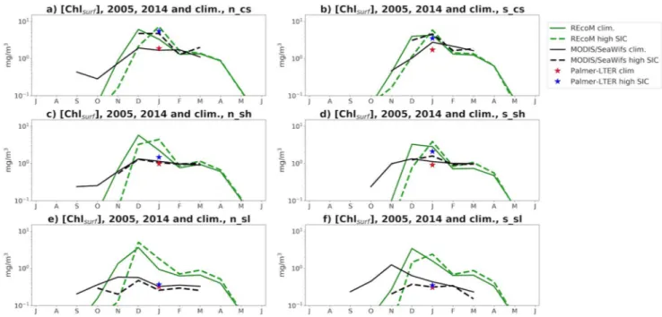
To compare the differences between years of early sea-ice retreat and the climatology, the monthly geomet- ric mean surface chlorophyll concentration for the early sea-ice retreat seasons (1998–1999, 2008–2009) were calculated for the satellite and model data and plotted against the monthly climatology (Figure 6).
The Palmer LTER data are considered as a January mean and is also plotted in the same figure. The model output suggests an earlier bloom compared to the climatology in the years of early sea-ice retreat. In the satellite data, this trend is observed in the slope region, and hard to determine in the coastal region given the lack of data during the spring and early summer.
By January, however, all data sets agree that surface chlorophyll concentrations are generally lower than the climatological values, with the exception being that Palmer LTER shows slightly higher concentrations in the northern slope and the satellite data has similar values to the climatology in the northern shelf. In the model, lower chlorophyll values in January can be attributed to iron limitation, given that an earlier bloom leads to earlier depletion (Figure S2). Although the model tends to underestimate MLD (Schultz et al., 2020), the time at which light limitation is lifted, associated with the sea-ice retreat, is well repre- sented. It is possible that the simulated shallower MLD contributes to less light limitation at the bottom of the mixed layer, contributing to the higher chlorophyll values compared to observations. In 2011, however, deeper than usual MLD due to very early sea-ice retreat was observed in the coastal and shelf areas during the Palmer LTER cruise (Schultz et al., 2020), associated with high chlorophyll and dFe concentrations
(Annett et al., 2017). The cruise data therefore indicates that although light limitation has a large role in controlling the timing of the bloom, there is enough PAR in mid-summer to fuel large primary production even in years of anomalously deep mixed layer, and iron limitation could be the reason for the lower con- centrations observed. While winter and spring data are not available from observations, simulated MLD (Figure S6) indicates that 2011 had anomalously high MLD throughout the winter and spring as well, even when compared to other early sea ice retreat years.
During the years of late sea-ice retreat (2004–2005, 2013–2014, Figure 7), it is hard to determine the time of the start of the bloom in the satellite data, given that chlorophyll cannot be observed earlier in the season due to sea-ice cover. During December and January, however, the satellite data shows that chlorophyll con- centrations are higher than their climatologies in the coastal region and southern shelf, with values similar to the climatology in the northern shelf and lower concentrations in the slope region. The Palmer-LTER and model data indicate higher chlorophyll in all sub-regions by January. In the model, this is due to a late start of the bloom, leading to a later peak.
Overall, despite disagreements in the mean chlorophyll values, all the data sets agree that the years with ear- ly sea-ice retreat had lower chlorophyll concentrations in January while late sea-ice retreat leads to higher chlorophyll concentrations. While difficult to assess the progression of the bloom in each set of years from the satellite and cruise data, the model indicates that less sea ice leads to an earlier bloom and less dFe avail- able by January, with the opposite happening in years of increased sea ice. While the timing of the bloom is dictated by PAR limitation, the summer concentrations depend on how much dFe has been consumed earlier in the season.
3.5. Spatial Distribution and Interannual Variability of DIC
January monthly mean surface DIC concentrations from the model output were compared to the Palmer LTER cruise data (Figure 8), with the anomalies relative to the climatology for each sub-region also shown.
The model is able to capture the onshore-offshore DIC gradient seen in the observations, with lower con- centrations toward the coast (Hauri et al., 2015). However, the simulated values have a bias toward lower concentrations compared to the cruise data. There are a few limitations in the model that could explain the Figure 6. MITgcm-REcoM2 (green) and MODIS/SeaWifs (black) log10-transformed climatological monthly surface chlorophyll concentration (full line) and mean concentration for years of early sea ice retreat (dashed line); Palmer-LTER log-transformed climatological surface chlorophyll concentration (red star, plotted as January mean) and mean for years of early sea ice retreat (blue star), during July–June, for regions n_cs (a), s_cs (b), n_sh (c), s_sh (d), n_sl (e), and s_sl (f).
low bias, one of them being that freshwater inputs are added at the surface, which could lead to less mixing and lower DIC from dilution. Also, the initial and boundary conditions are based on gridded data sets that are derived from observations mostly collected in open-ocean locations, and Jones et al. (2017) found that DIC concentrations in Antarctic Circumpolar Water (ACC) derived water masses were higher in the shelf due to respiration and remineralization as the water mass makes its way from the slope to the coast. When compared to observations, the model shows a bias toward higher NPP, which could lead to more carbon uptake and contribute to the lower DIC values in the simulation.
Despite a bias toward lower concentrations, the interannual variability of simulated DIC is similar to the variability observed in the Palmer LTER cruise data in most regions, with the exception of the southern slope (Table S2). DIC variations throughout the season are influenced by a series of physical and biological mechanisms (Ducklow et al., 2018). The variability of the physical mechanisms that affect DIC concentra- tions, which are deepening of the MLD (which leads to entrainment of high-DIC sub-surface waters) and sea ice melt (which leads to dilution), are well represented in the model (Schultz et al., 2020). Although the phytoplankton bloom is patchy and chlorophyll concentration varies throughout the season at individual locations, the biological signature of net community production carbon uptake lasts throughout the growth season (September to the Palmer LTER survey cruise in January). Therefore, the better agreement between simulated and cruise DIC values compared to the chlorophyll concentration adds to the evidence that part of the disagreement between the chlorophyll data sets is due to the patchiness of the data, and that integrat- ed over the season, the biological processes are better represented in the model.
Some of the discrepancies between simulated and cruise DIC are likely to be due to the same mechanisms as the discrepancies in the chlorophyll values. In 2011, the model was not capable of capturing the large bloom observed, leading to positive DIC anomalies in the southern region while the cruise data shows neg- ative anomalies. For the years of early sea-ice retreat analyzed, both REcoM2 and Palmer-LTER data show positive DIC anomalies, while for the years of late sea-ice retreat the anomalies are mostly negative with the exception of the slope region.
Figure 7. MITgcm-REcoM2 (green) and MODIS/SeaWifs (black) log10-transformed climatological monthly surface chlorophyll concentration (full line) and mean concentration for years of late sea-ice retreat (dashed line); Palmer-LTER log10-transformed climatological surface chlorophyll concentration (red star, plotted as January mean) and mean for years of early sea-ice retreat (blue star), during July-June, for regions n_cs (a), s_cs (b), n_sh (c), s_sh (d), n_sl (e), and s_sl (f). Vertical lines represent standard deviation.
3.6. DIC-Derived Net Community Production
Although the DIC anomalies provide an indication of the physical and biological processes that took place throughout the growth season, further quantification is needed to assess how much of the DIC drawdown is due to net biological uptake, air-sea fluxes, and sea ice melt. The calculations described in Section 2.4 provide an estimate of the influence of each of these processes in the DIC, and the total DIC drawdown, air- sea CO2 fluxes, DIC dilution due to sea ice melt, NCP and seasonally integrated NPP (a diagnostic variable) are shown, for each sub-region, on Figure 9. January NPP is shown in Figure S4. All these figures include the calculations for the climatology and for the years of early and late sea-ice retreat described in previous sections.
In a study using Palmer LTER cruise data, Ducklow et al. (2018) find that NCP is significantly higher than measured export flux, a conclusion that is also reached by other studies (Buessler et al., 2010; Stukel et al., 2015; Weston et al., 2013). Within each year sampled, the variability of each rate process measured, including NCP, was moderately high in both space and time and production likely being higher in sunny Figure 8. Palmer-LTER (left) and MITgcm-REcoM2 (right) January surface DIC concentrations (a, b, e, and f) for north (a and b) and south (e and f) regions;
and anomalies relative to the mean (January mean for simulated, and cruise mean for Palmer-LTER, c, d, g, and h).
days (vs. cloudy conditions). The authors also point out that one of the big uncertainties in trying to assess the relative magnitude of each estimate is the difficulty in specifying the start of the growing season after sea-ice retreats.
Total DIC drawdown is highest in the shelf and coastal areas during years of late sea-ice retreat, compared to the climatology and to years of early sea-ice retreat (Figures 9a and 9b). This happens despite NCP being higher in years of early sea-ice retreat throughout the whole grid (Figures 9g and 9h). The largest drawdown was observed in the northern coast, with a climatological decrease of 4.86 molC/m2 during the season that reached 5.65 molC/m2 during years of late sea-ice retreat. Higher NCP in years of low SIC is consistent with the satellite estimates of Li et al. (2016), who found that variations in NCP were linked to sea ice, and that annually integrated NCP was higher with higher sea surface temperature and longer bloom season. The larger DIC drawdown despite lower NCP indicates a strong influence of physics in the inorganic carbon cy- cle. With increased sea ice throughout the season, there is less air-sea transfers (which are a source of DIC) and more dilution by late summer. It is worth noting that in Ryder Bay, Rozema et al. (2017) observed lower phytoplankton biomass following years of low sea ice concentration during the winter. Coastal stations such as Ryder Bay, however, are more influenced by phenomena that are not captured by the model (such Figure 9. Seasonally integrated (between September and January) total vertically integrated DIC drawdown (a and b), air-sea CO2 flux (c and d), effect of sea-ice melt on DIC concentration (e and f), DIC-derived NCP corrected for air-sea flux, and sea ice melt (g and h) and NPP (i and j) for the northern (left) and southern (right) regions. The sign reflects the effect on the DIC inventory, so that positive FCO2 reflects a flux into the ocean and negative meltwater influence reflects dilution. Shown for climatology (black), years of early sea-ice retreat (red, 1998–1999, 2008–2009), and years of late sea-ice retreat (blue, 2004–2005, 2013–2014).
as the passage of icebergs and the strong stratification near sea ice), and can have different responses than the observed in the shelf and even in the coastal regions as defined in this study.
In previous studies using Palmer LTER cruise data, Hauri et al. (2015) found that DIC spatial variability dur- ing the summer was driven by increased biological activity in the south of the WAP and by increased melt- water toward the north, and Eveleth, Cassar, Doney, et al. (2017) and Eveleth, Cassar, Sherrell, et al. (2017) found that physical processes had a more pronounced influence in the southern onshore region where active sea-ice melt was still happening. The model results show that although climatological summer melt- water values (December–February) are higher in the southern part of the grid (Schultz et al., 2020), inte- grated over spring and summer sea-ice melt has a larger influence in the northern WAP in years of late sea-ice retreat, and larger influence in the southern part in years of early sea ice retreat (Figures 9e and 9f).
The calculation performed to account for the influence of meltwater takes into account the depth of the MLD, which is shallower in the northern part of the grid (Schultz et al., 2020), increasing the effect of melt.
Both sea-ice melt and primary production tend to be higher in the southern part of the grid by January and February when the Palmer LTER cruise takes place, but the relative importance of each process varies from year to year.
Evidence that both biological and physical processes can lead to anomalously high DIC drawdown is seen in the shelf sub-regions, where both years of early and late sea-ice retreat show more DIC drawdown than the climatological values. In years of early retreat, the low dilution by meltwater and increased DIC input by air-sea CO2 fluxes is compensated by the higher NCP, which reaches values as high as 6.52 molC/m2 in the northern shelf. In years of high SIC, however, low air-sea fluxes and higher meltwater content keep the DIC drawdown below climatological values despite the low NCP. The WAP is a sink of atmospheric carbon throughout the season in all years, but the amount of carbon the ocean uptakes depends on the duration of the ice-free season.
Years of high SIC show higher productivity in January, and overall higher DIC drawdown. If NPP and NCP are integrated over the spring and summer seasons, however, it is seen that this is because of the timing of the bloom associated with the effect of physics in the DIC drawdown, not because of higher productivity.
While January high chlorophyll values are accompanied by larger DIC drawdowns, these effects are not directly linked, although they are both driven by the timing and magnitude of sea-ice melt. Years of low SIC also show more DIC drawdown than the climatology, driven by the higher NCP throughout the season.
Despite the high NCP, years of early sea-ice retreat still show positive DIC anomalies in January. The anom- alies, however, reflect the positive anomalies that are observed at the beginning of the season (Figure S5), which are also positive possibly due to increased mixing with DIC-rich subsurface waters under lower SIC.
4. Discussion and Conclusions
The MITgcm-REcoM2 model implemented for the WAP is able to represent the main patterns observed in the phytoplankton bloom, such as higher concentrations onshore and progression of the bloom from north to south and offshore to onshore. The onshore-offshore chlorophyll gradient seen in the observations, however, is not as pronounced in the model simulation. Li et al. (2016) find that the annually integrated net community production (NCP) in the coastal areas is up to 8 times higher than what is observed offshore, and Vernet et al. (2008) finds that primary production ranges from 500 to 750 mgC/m2d shoreward of the continental slope and from 250 to 400 mgC/m2d over the slope region. In the model, January NPP is 3.05 times higher in the coastal region (compared to the slope) in the northern region, and 2.62 times higher in the southern region. Integrated over September–January, however, the whole grid shows comparable NPP.
Comparing chlorophyll values among the different data sets (cruise, satellite, and model) is challenging given that the phytoplankton bloom in the WAP is highly variable and patchy, and there are gaps in the temporal and spatial coverage of the observations. Some of the discrepancies observed between data sets in the chlorophyll anomalies, therefore, are likely attributable to timing of the sampling. DIC anomalies in mid-summer, on the other hand, are the result of the cumulative effect of processes that took place throughout the season. The model captures well the climatological spatial pattern in the summer surface DIC field with larger seasonal drawdown and dilution onshore, and the model is able to reproduce much of the interannual variability seen in the DIC measurements from the Palmer LTER cruises. While in the
model, MLD variability is not well represented in the southern slope and northern coast, it is reasonably well represented in most of the grid, especially in the shelf region (Schultz et al., 2020). The model also has a good representation of sea ice variability and correctly predicts higher seasonally integrated productivity in years of low SIC. We therefore use the model results to estimate the importance of biological and physical processes in driving DIC drawdown each year.
In years of early sea-ice retreat, both observations (satellite and cruise) and model data show lower chloro- phyll concentrations in January compared to the climatology. While January NPP is also lower than clima- tology, seasonally integrated NPP (September to January) is higher, with a longer productive season due to light limitation being lifted earlier. Surface DIC drawdown during the same period, however, is lower de- spite the increased NPP. This can be attributed to the increased air-sea CO2 fluxes and to decreased dilution by sea ice melt. Years of late sea-ice retreat, on the other hand, show higher than climatological chlorophyll concentrations in January in all the data sets analyzed. The model results indicate that these years exhibit NPP higher than the climatology for January, but overall less seasonally integrated NPP. The longer sea-ice season also leads to a smaller sink of atmospheric CO2 and increased influence of sea-ice melt, resulting in larger DIC drawdown between September and January.
Although it is hard to estimate when the bloom starts in the satellite data due to cloud and sea-ice cover, in the model results, the January chlorophyll concentration anomalies are a result of the timing of the bloom;
with late sea-ice retreat, the light limitation is lifted later in the year and the bloom is closer to its peak in January, while early sea-ice retreat leads to an earlier bloom and a weaker phytoplankton bloom in January, with the productivity decreasing due to lower iron concentrations. The model results are consistent with DIC concentrations deviating from the dilution curve, with lower concentrations than expected, in January during years of high chlorophyll concentrations as found in Hauri et al. (2015), but our results suggest that sea-ice melt also plays an important role in driving the seasonal DIC drawdown. Air-sea CO2 fluxes have a much larger influence in counteracting the drawdown by biological activity in years of early sea-ice retreat, due to longer ice-free season.
Since ocean dissolved iron (dFe) data is scarce, building initial and boundary conditions for this micronutri- ent is a challenge. Given that iron is thought to be the limiting factor offshore, and that complete iron lim- itation is not encountered in the model, we suspect that the initial and boundary conditions overestimate dFe, which is supplied in excess in the offshore region due to mixing with iron-rich subsurface waters. The lack of iron data is not only a limitation to build reliable forcings for the model, but also to understand the mechanisms governing the phytoplankton spatial and temporal variability in the WAP. The role of differ- ent sources of dFe in the WAP biogeochemistry, therefore, is a question that requires future research and increased field sampling.
Interannual variability of glacial sources of freshwater and dFe are also missing. Although there is substan- tial melting of glacial waters on the continent, most of it freeze before reaching the ocean (Van Wessem et al., 2016). The re-freezing of glacial melt impedes the estimation of yearly runoff to the ocean, although a climatology can be obtained using the mass balance over a larger time scale. Some of the discrepancies in chlorophyll concentration between model and data are attributed to the lack of interannual variability in the glacial dFe input. In 2011, Annett et al. (2017) found anomalously high dFe concentrations linked to increased glacial meltwater, which in turn led to large and positive chlorophyll anomalies. This was a warm year with very early sea-ice retreat, and the high chlorophyll concentration differs from what is observed in other years of early SIC retreat (decreasing bloom by January). It seems likely, therefore, that 2011 was indeed an anomalous year with high glacial input leading to a large sustained bloom, and that the lack of interannual variability in the glacial inputs in the model prevented it from representing the high bloom.
Sherrell et al. (2018) found that dFe near Palmer Deep (on the northern, coastal part of the grid) is provided by sediment sources in coastal, shallower areas, which is then advected to the shelf region. The authors also argue that the difference from the hypothesis proposed by Annett et al. (2017), that dFe is mostly from glacial origin, could be due to regional differences or due to errors in the data interpretation of Annett et al. (2017), which would be caused by vertical mixing weakening the 18O isotope signature used to estimate the origin of the freshwater in that study. The model results suggest that sediment sources of dFe are impor- tant in the coastal regions, and that part of the dFe in the northern shelf is also of sedimentary origin. In the