Supporting Information for ’Phytoplankton blooms at
1
increasing levels of atmospheric carbon dioxide:
2
experimental evidence for negative effects on
3
prymnesiophytes and positive on small
4
picoeukaryotes’
5
S-3 Methods
6
S-3.1 pH dye preparation, measurements and corrections
7
Determination of seawater pH followed in principle the spectrophotometrical approach of
8
Clayton and Byrne (1993) described in Dickson, A. G. and Sabine, C. L. and Christian, J.R.
9
(Eds.) (2007) making use of the dye m-cresol purple (Acros Organics, CAS 62625-31-4, Lot
10
A026431) at 25◦C in a 10 cm thermostated cuvette on a Cary 100 (Varian). Concerning the
11
dye, 300 ml of an about 2 mM solution was prepared in Milli-Q, the ionic strength brought to
12
0.66 with NaCl (matching that of seawater with a salinity of ∼32) and the pHT (pH on the
13
total scale) adjusted to about 7.6 (at 25◦C). After that the solution was sterile filtered (0.2µm)
14
into a gas and light impermeable sampling bag (Supelco), filled without air.
15
For measurements, 5 ml of sample water was pumped from the bottom of a 100 ml bottle,
16
brought to 25◦C in a thermostated water bath, into a 25 ml syringe pump (Tecan, Cavro XLP
17
6000), followed by about 50 µl of m-cresol purple dye solution, and then mixed within the
18
syringe with an additional 15 ml of sample water. This mixture was then injected into the
19
10 cm flow-through cuvette (with a capacity of about 8 ml), which had been previously filled
20
carefully whiteout air bubbles with filtered (0.2µm) fjord water, or already contained sample
21
water. Samples were measured from low to high fCO2, and potential carry-over from a previ-
22
ous sample was usually below detection limit. Each seawater sample was measured in triplic-
23
ates and precision of replicate measurements was typically 0.001 or better for the higher and
24
0.002 or better for the lower pH treatments (with the threshold at an in situ pH of about 7.700).
25
Measured absorption spectra (780 to 380 nm at 1nm resolution and a scan rate of 600 nm per
26
minute) were corrected for tiny air bubble entrainment by comparison to an absorption mean
27
between 735 and 725 nm, wavelengths at which the dye is non-absorbent, of a baseline in
28
Milli-Q. The resulting absorption ratio at 578 and 434 nm was then used to calculatepHT us-
29
ing the acid dissociation constant and extinction coefficient ratios of m-cresol purple reported
30
in Dickson, A. G. and Sabine, C. L. and Christian, J.R. (Eds.) (2007). Furthermore, absorb-
31
ance at 578 nm, the isosbestic point, was used to correct the calculated pH by accounting for
32
inevitable changes due to dye addition (about -0.005 pH units at the highest and +0.014 at
33
the lowest pH), similar to the method described in Clayton and Byrne (1993). For that pur-
34
pose five seawater batches of different pH, one liter each, covering the entire measurement
35
range, were prepared, and in each pH was determined as described above, but with increasing
36
amounts of dye (six levels). At each pH level a linear correlation between the change in pH in
37
relation to the absorbance at the isosbestic point (a measure for the amount of dye added) was
38
constructed. The combination of all six correlations at each pH level then led to an uniform
39
linear relation describing the change in measured pH in response to a certain amount of dye
40
added at a certain pH.
41
To assess the accuracy of pH measurements, and to account for potential impurities in the
42
m-cresol purple sodium salt, pHT was measured and corrected as described above on five
43
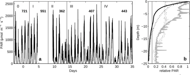
replicates of CRM batch 108 (freshly opened). However, no further corrections were applied
44
as measuredpHT (7.8791±0.0002) was off less then 0.001 units the theoretical one of 7.8786,
45
calculated from known DIC (2022.7 µmol kg−1), total alkalinity, TA (2218.0 µmol kg−1),
46
salinity (33.224), phosphate (0.41 µmol kg−1) and silicate (2.9 µmol kg−1) concentrations
47
using the dissociation constants for carbonic acid from Mehrbach et al. (1973) as refitted by
48
Lueker et al. (2000).
49
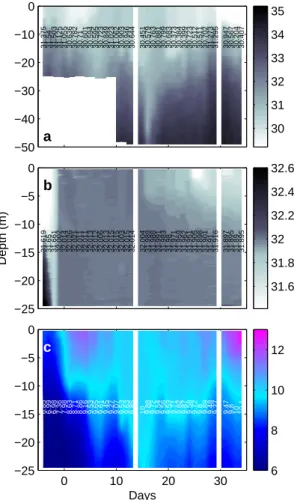
S-3.2 pH sample filtration
50
Prior to analysis samples for pH were transferred from the 500 ml glass stoppered bottles
51
(Schott Duran) with a membrane pump to 100 ml glass stoppered bottles (Schott Duran) at a
52
flow rate of about 50 ml per minute, passing a sterile 0.2µm filter (Sarstedt Filtropur, PES
53
membrane). For that the sample water was pumped from the bottom of the 500 ml bottles,
54
filling the 100 ml bottles through a serological needle from bottom to top with about 100 ml
55
of additional overflow. Since about 300 ml of sample water always remained in the larger
56
bottles, tubing was Tygon and the smaller bottles were filled from bottom to top with consider-
57
able overflow, potentialCO2 gas exchange with the atmosphere, impacting seawater pH, was
58
minimized. Filtration removed all particulate organic matter which, at relatively high concen-
59
trations, can influence the precision of spectrophotometric measurements. Furthermore, the
60
close to sterile seawater samples are relatively stable as potential biological activity by phyto-
61
plankton or bacteria, otherwise impacting pH, is minimized. The 100 ml bottles were closed
62
without headspace and, if not measured within the next couple of hours, stored at4◦C in the
63
dark.
64
S-3.3 Carbonate chemistry calculations
65
In a first step measuredpHT (at 25◦C) and DIC was used to calculate practical alkalinity (PA).
66
The second step involved calculatingpHT and all the other carbonate chemistry components
67
such as the fugacity of carbon dioxide, fCO2, at in-situ temperature and salinity conditions
68
from measured DIC and calculated PA, using the dissociation constants for carbonic acid
69
from Mehrbach et al. (1973) as refitted by Lueker et al. (2000). Since there were no DIC and
70
spectrophotometric pH measurements on the first three (t-3 to t-1) and last six days (28 to 34),
71
carbonate chemistry speciation had to be estimated using CTD-derived mean water column
72
pH measurements, brought to the total scale with CTD to spectrophotometric pH relations
73
for day 0 and 27 (compare section 3.5), and salinity based estimates of PA. For that purpose,
74
mean water column salinity changes were considered a proxy for changes in PA, taking a mean
75
initial PA of 2180 µmol kg−1 and a mean initial salinity of 31.95. The assumption that the
76
sole drivers of TA changes are freshwater input by rain and evaporation obviously ignores the
77
impact of phosphate and nitrate assimilation and calcium carbonate production on TA. Never-
78
theless, here estimates of carbonate chemistry speciation will hardly be affected as 1) changes
79
in alkalinity due to nutrient assimilation (about +5µmol kg−1) and calcification (maximum
80
of -2µmol kg−1), which furthermore work in opposite directions, were smaller than those by
81
freshwater input (about -9µmol kg−1) and 2) the estimates are based on measured pH, ren-
82
dering the carbonate system practically insensitive to even relatively large PA uncertainties
83
(depending on actualCO2 level, 10µmol kg−1 correspond to only a fewµatm).
84
S-4 Results
85
S-4.1 Changes in light, salinity and temperature
86
Average incident photosynthetic active radiation (PAR) measured in air was similar during all
87
phases, although slightly higher during the first two weeks (Fig. S-3). Light profiles taken
88
within and outside the mesocosms were generally very similar, with marginally higher atten-
89
uation in the upper 10 m of the mesocosms, possibly due to shading by the floating structures,
90
and potentially higher particulate biomass (Fig. S-3b). Nevertheless, no significant differ-
91
ences were observed between mesocosms and through time (data not shown), while attenu-
92
ation coefficients were similar in comparison to a previous KOSMOS study, with typicalkd
93
values between 0.3 and 0.4 (Schulz et al., 2013). Using an average incident PAR intensity
94
of 450µmol m−2s−1 during daylight, depth-averaged (0.3-23 m) light conditions were about
95
56µmol m−2s−1. This is probably at least three times lower then in two previous mesocosm
96
experiments at the same location in bags of only 5 (Engel et al., 2005) and 10 meters depth
97
Schulz et al. (2008).
98
Depth-averaged salinity in the fjord ranged from 30.20 to 31.54, thus being more variable
99
than in the mesocosms (Fig. S-2a). Ignoring the initial salt addition for volume determinations,
100
depth-integrated variability within the mesocosms was about 0.15 salinity units, and while
101
being relatively stable throughout the first 2 weeks, constantly decreased towards the end of
102
the experiment. This decrease was most likely due to rain water input as most pronounced
103
in the upper 5-10 m of the mesocosms (Fig. S-2b). Overall dilution by rainwater was on the
104
order of 5h.
105
Average water column temperatures steadily increased within the mesocosms and the fjord,
106
from initially about 7 to 10◦C half way through the experiment (Fig S-2c). Although surface
107
waters continued to warm, upwelling of colder deeper waters in the fjord to up to 15 m depth,
108
also mirrored in salinity changes (Fig S-2a), kept average temperatures relatively constant
109
until the end of the experiment. Average temperatures did not significantly exceed 10◦C, and
110
reached up to 13◦C in the upper meter by the end of the experiment Fig S-2c).
111
References
112
Clayton, T. D. and Byrne, R. H. (1993). Spectrophotometric seawater pH measurements: total
113
hydrogen ion concentration scale calibrations of m-cresol purple and at-sea results. Deep-
114
Sea Res. 40, 2115–2129
115
Dickson, A. G. and Sabine, C. L. and Christian, J.R. (Eds.) (2007). Guide to Best Practices for
116
OceanCO2 Measurements. PICES Special Publication 3
117
Engel, A., Zondervan, I., Aerts, K., Beaufort, L., Benthien, A., Chou, L., et al. (2005). Testing
118
the direct effect ofCO2 concentration on a bloom of the coccolithophorid Emiliania huxleyi
119
in mesocosm experiments. Limnol. Oceanogr. 50, 493–507
120
Lueker, T. J., Dickson, A. G., and Keeling, C. D. (2000). Ocean pCO2calculated from dissolved
121
inorganic carbon, alkalinity, and equations for K1 and K2: validation based on laboratory
122
measurements ofCO2 in gas and seawater at equilibrium . Mar. Chem. 70, 105–119
123
Mehrbach, C., Culberson, C. H., Hawley, J. E., and Pytkowicz, R. M. (1973). Measurements
124
of the apparent dissociation constants of carbonic acid in seawater at atmospheric pressure.
125
Limnol. Oceanogr. 18, 897–907
126
Schulz, K. G., Bellerby, R. G. J., Brussaard, C. P. D., B¨udenebnder, J., Czerny, J., Engel, A., et al.
127
(2013). Temporal biomass dynamics of an Arctic plankton bloom in response to increasing
128
levels of atmospheric carbon dioxide. Biogeosci. 10, 161–180
129
Schulz, K. G., Riebesell, U., Bellerby, R. G. J., Biswas, H., Meyer¨ofer, M., M¨uller, M. N., et al.
130
(2008). Build-up and decline of organic matter during PeECE III. Biogeosci. 5, 707–718
131
TableS-1:R2 ,Fandpvaluesforstatisticallysignificantcorrelations(p<0.05)betweenthemeanofameasurementparameter andfCO2duringacertainphaseoftheexperiment.Fordetailsseesection3.8.Positivecorrelationsareshowninbold, negativeinitalic(intotal60outof160).Superscriptsa ,b ,c ,d ,andf refertodatashowninFigs.3,S-5,4,5,S-6, respectively PhaseIPhaseIIPhaseIIIPhaseIV adj.R2 Fpadj.R2 Fpadj.R2 Fpadj.R2 Fp a,d Chla0.759823.140.0030.673415.430.008 b POC0.700215.020.012 b PON0.51208.340.028 b POP0.758322.960.0030.756122.700.003 b BSi b DOC0.50418.120.029 b DON b DOP0.52688.790.0250.52608.770.025 a Nitrate0.41996.070.049 a Ammonia0.763323.570.0030.803729.660.002 a Phosphate0.55799.8350.020 a Silicate a ∆[O2]0.602711.620.0140.736020.510.004
ab.continued PhaseIPhaseIIPhaseIIIPhaseIV adj.R2 Fpadj.R2 Fpadj.R2 Fpadj.R2 Fp c ChlaHapto0.821533.230.0010.44516.620.0420.803229.560.002 c ChlaChryso0.52878.850.025 c ChlaDino c ChlaDiatom0.699817.310.006 c ChlaChloro0.905568.06<0.0010.845439.27<0.0010.665614.930.0080.52388.700.026 c ChlaCrypto0.764623.740.003 c ChlaCyano0.46136.990.0380.773924.970.0030.9391108.9<0.0010.798428.730.002 d SynFCM0.563310.030.0190.48207.520.0340.921282.81<0.0010.729219.850.004 d PicoFCM0.859043.63<0.0010.9560153.15<0.0010.894860.56<0.0010.687916.430.007 d EhuxFCM0.680515.920.0070.46317.040.0380.44126.530.043 d NanosmallFCM0.51378.390.030 d NanobigFCM0.593611.230.0150.870247.93<0.001 d CryptoFCM0.661414.670.009 e HaptoMicro0.695216.960.0060.587410.960.016n.a.n.a.n.a. e DinoNTMicro0.636613.260.011n.a.n.a.n.a. e DinoTMicron.a.n.a.n.a. f DiatomMicro0.770724.520.003n.a.n.a.n.a. e ChloroMicro0.624612.650.012n.a.n.a.n.a. e CryptoMicron.a.n.a.n.a. e DinoHTMicro0.51718.500.027n.a.n.a.n.a. e Tot.autoMicro0.842236.36<0.001n.a.n.a.n.a.
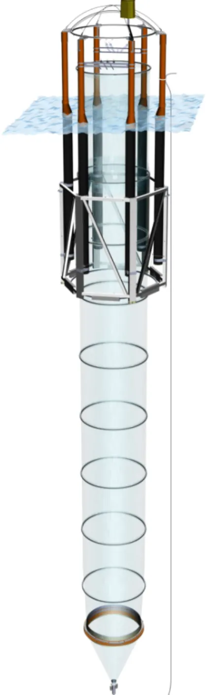
Figure S-1: Schematic drawing of a KOSMOS mesocosm deployed in Raunefjorden, Nor- way. The orange flanges at depth connect the funnel-shaped sediment trap to the rest of the bag.
−25
−20
−15
−10
−5 0
31.619 31.65 31.661 32.002 32.014 32.026 32.021 32.011 32.011 32.013 32.012 32.006 32.013 32.015 32.015 32.003 32.015 32.014 32.004 31.989 31.988 31.991 31.983 31.98 31.971 31.959 31.962 31.951 31.905 31.898 31.901 31.91 31.916 31.897 31.895 31.89 31.895
b
Depth (m)
31.6 31.8 32 32.2 32.4 32.6
−50
−40
−30
−20
−10 0
31.375 31.54 31.503 31.125 31.055 30.636 30.782 30.71 30.601 30.594 30.595 30.723 30.849 31.023 31.062 30.903 30.946 30.644 30.451 30.579 30.763 30.881 30.799 30.683 30.373 30.384 30.399 30.723 30.512 30.511 30.702 31.273 31.295 30.947 30.567 30.204 30.407
a 30
31 32 33 34 35
0 10 20 30
−25
−20
−15
−10
−5 0
6.85 6.99 6.98 7.36 7.98 8.63 8.71 8.86 9.16 9.53 9.65 9.61 9.45 9.27 9.07 9.53 9.63 9.85 10 9.88 9.72 9.54 9.56 9.53 9.71 9.82 9.87 9.58 9.72 9.8 9.89 9.48 9.27 9.47 9.8 10 10.1
c
Days
6 8 10 12
Figure S-2: Vertical distribution and dynamics of salinity measured in the fjord (a) and meso- cosm M9 (b) together with those of temperature (c), given in degrees Celsius.
Note that with the exception of mesocosm M2 which had a hole right from the beginning, allowing fjord and mesocosm water to exchange, temperature and sa- linity dynamics in all other mesocosms were practically identical. Numbers rep- resent depth-averaged (0.3-23 m) values.
0 5 10 15 20 25 30 35 0
500 1000 1500 2000 2500
Days PAR (µmol m−2 s−1 )
0 I II III IV
721 551 362 407 443
a
0 0.2 0.4 0.6 0.8 1
−25
−20
−15
−10
−5 0
relative PAR
Depth (m)
b
Turbidity (kg m−3)
Figure S-3: (a) Changes in photosynthetic active radiation (PAR) in air, and (b) a typical ver- tical light (black) and turbidity (grey) profile in a mesocosm (solid lines) and the fjord (dotted lines). Numbers in (a) denote average daily PAR levels during a cer- tain phase, indicated by vertical lines and Roman numbers. In (b) the vertical line marks the 10% level of incident light. For details on measurements see section 3.5.
−25
−20
−15
−10
−5 0
M1
8.11 8.09 8.07 8.09 8.12 7.97 7.8 7.75 7.76 7.72 7.7 7.73 7.76 7.76 NaN 7.75 7.78 7.79 7.78 7.78 7.81 7.81 7.84 7.86 7.86 7.85 7.86 7.87 7.87 7.85 7.86 7.87 7.87 7.89 7.87 7.87 7.88 8.16 8.1 8.06 8.08 8.11 7.96 7.78 7.74 7.77 7.73 7.72 7.77 7.79 7.79 7.82 7.81 7.82 7.82 7.82 7.85 7.91 7.93 7.95 7.95 7.96 7.95 7.97 7.96 7.95 7.94 7.94 7.97 7.97 8 7.99 7.98 7.99
8.06 8.07 8.07 8.09 8.12 8 7.83 7.76 7.76 7.71 7.69 7.7 7.73 7.73 NaN 7.71 7.75 7.75 7.75 7.75 7.76 7.75 7.76 7.78 7.77 7.76 7.78 7.79 7.81 7.79 7.8 7.81 7.81 7.81 7.8 7.8 7.79
Depth (m)
−25
−20
−15
−10
−5 0
M2
8.11 8.1 8.07 8.09 8.13 8.12 8.13 8.14 8.13 8.13 8.13 8.12 8.13 8.14 8.13 8.12 8.12 8.14 8.11 8.12 8.12 8.12 8.15 8.15 8.15 8.15 8.15 8.15 8.14 8.15 8.14 8.15 8.13 8.14 8.15 8.13 NaN 8.15 8.11 8.06 8.08 8.13 8.13 8.14 8.15 8.15 8.15 8.15 8.14 8.14 8.16 8.15 8.15 8.13 8.16 8.13 8.14 8.15 8.17 8.2 8.2 8.2 8.2 8.2 8.19 8.18 8.19 8.17 8.21 8.17 8.19 8.2 8.19 NaN
8.07 8.07 8.07 8.08 8.13 8.11 8.12 8.12 8.11 8.11 8.1 8.1 8.11 8.12 8.12 8.1 8.1 8.11 8.1 8.11 8.1 8.1 8.11 8.11 8.1 8.1 8.11 8.11 8.11 8.11 8.1 8.11 8.09 8.11 8.11 8.09 NaN
M3
8.12 8.1 8.08 8.06 8.12 7.98 7.8 7.68 7.69 7.61 7.62 7.62 7.66 7.65 7.66 7.65 7.67 7.68 7.69 7.71 7.73 7.73 7.75 7.78 7.77 7.78 7.8 7.81 7.81 7.82 7.81 7.8 7.78 7.79 7.81 7.79 7.79 8.16 8.12 8.07 8.06 8.12 7.97 7.78 7.66 7.69 7.61 7.64 7.67 7.7 7.69 7.72 7.73 7.72 7.73 7.75 7.81 7.84 7.86 7.87 7.88 7.9 7.92 7.94 7.94 7.93 7.92 7.94 7.95 7.92 7.95 7.95 7.93 7.94
8.07 8.08 8.09 8.06 8.12 7.99 7.84 7.7 7.69 7.61 7.6 7.6 7.63 7.62 7.62 7.61 7.62 7.63 7.66 7.66 7.67 7.65 7.67 7.69 7.67 7.67 7.69 7.72 7.73 7.76 7.72 7.71 7.7 7.7 7.71 7.69 7.69
M4
8.09 8.07 8.06 8.06 8.13 8.1 8.11 8.13 8.12 8.12 8.12 8.12 8.12 8.14 8.13 8.12 8.12 8.11 8.1 8.13 8.11 8.13 8.13 8.13 8.13 8.14 8.15 8.15 8.14 8.13 8.14 8.15 8.13 8.14 8.14 8.13 8.13 8.15 8.08 8.05 8.06 8.13 8.1 8.12 8.14 8.14 8.14 8.15 8.14 8.13 8.15 8.14 8.14 8.12 8.12 8.1 8.14 8.12 8.16 8.17 8.16 8.18 8.18 8.2 8.19 8.18 8.18 8.17 8.19 8.15 8.18 8.17 8.16 8.17
8.05 8.06 8.06 8.07 8.13 8.09 8.1 8.11 8.1 8.1 8.1 8.1 8.1 8.12 8.12 8.11 8.11 8.1 8.09 8.12 8.1 8.12 8.11 8.1 8.1 8.11 8.12 8.12 8.11 8.11 8.11 8.12 8.1 8.11 8.11 8.1 8.1
M5
8.1 8.08 8.06 8.05 8.11 7.97 7.8 7.63 7.56 7.51 7.54 7.55 7.59 7.58 7.6 7.6 7.62 7.62 7.64 7.68 7.68 7.69 7.7 7.72 7.71 7.72 7.74 7.75 7.77 7.74 7.75 7.77 7.75 7.77 7.76 7.75 7.76 8.16 8.1 8.05 8.05 8.11 7.96 7.77 7.6 7.55 7.52 7.56 7.62 7.65 7.64 7.67 7.72 7.69 7.7 7.73 7.82 7.83 7.85 7.85 7.84 7.87 7.9 7.93 7.93 7.93 7.92 7.92 7.96 7.93 7.95 7.94 7.92 7.94
8.05 8.05 8.06 8.06 8.12 7.98 7.84 7.66 7.58 7.52 NaN 7.52 7.55 7.54 7.55 7.54 7.56 7.55 7.59 7.62 7.6 7.6 7.61 7.63 7.6 7.6 7.62 7.63 7.66 7.63 7.64 7.65 7.64 7.65 7.64 7.63 7.64
M6
8.09 8.07 8.06 8.05 8.12 8.05 8.06 8.07 8.07 8.03 8.03 8.03 8.04 8.04 8.05 8.04 8.03 8.01 8.02 8.05 8.04 8.06 8.06 8.06 8.07 8.07 8.07 8.09 8.08 8.07 8.08 8.09 8.07 8.08 8.07 8.06 8.07 8.13 8.07 8.04 8.05 8.12 8.04 8.07 8.08 8.08 8.03 8.04 8.04 8.05 8.05 8.06 8.06 8.04 8.03 8.03 8.06 8.07 8.11 8.11 8.1 8.12 8.12 8.12 8.13 8.11 8.11 8.11 8.14 8.12 8.14 8.13 8.12 8.12
8.04 8.07 8.06 8.05 8.12 8.05 8.06 8.06 8.05 8.02 8.02 8.02 8.03 8.04 8.04 8.03 8.02 8 8.01 8.04 8.03 8.04 8.03 8.03 8.03 8.02 8.04 8.06 8.05 8.04 8.05 8.05 8.04 8.04 8.03 8.02 8.02
M7
8.09 8.08 8.05 8.06 8.13 7.99 7.84 7.59 7.41 7.36 7.38 7.4 7.44 7.43 7.46 7.45 7.49 7.5 7.52 7.56 7.57 7.57 7.62 7.63 7.63 7.64 7.65 7.65 7.68 7.65 7.66 7.67 7.66 7.65 7.66 7.64 7.65 8.14 8.1 8.05 8.06 8.13 7.98 7.83 7.58 7.4 7.38 7.41 7.48 7.5 7.51 7.53 7.57 7.56 7.57 7.62 7.73 7.76 7.78 7.81 7.78 7.82 7.83 7.83 7.82 7.84 7.83 7.84 7.88 7.85 7.83 7.84 7.82 7.85
8.04 8.06 8.05 8.06 8.13 8 7.86 7.6 7.42 7.37 7.38 7.37 7.4 7.39 7.41 7.39 7.42 7.43 7.47 7.48 7.47 7.47 7.5 7.51 7.5 7.5 7.51 7.53 7.56 7.52 7.55 7.54 7.55 7.54 7.54 7.52 7.53
M8
8.1 8.08 8.05 8.06 8.12 7.97 7.87 7.89 7.88 7.87 7.87 7.88 7.88 7.9 7.89 7.89 7.89 7.88 7.89 7.9 7.9 7.93 7.94 7.95 7.95 7.96 7.97 7.96 7.98 7.95 7.96 7.99 7.97 7.97 7.97 7.95 7.93 8.15 8.1 8.05 8.05 8.12 7.97 7.86 7.89 7.89 7.88 7.89 7.9 7.9 7.92 7.92 7.92 7.9 7.91 7.93 7.95 7.97 8.03 8.03 8.03 8.05 8.04 8.05 8.04 8.05 8.03 8.04 8.07 8.05 8.06 8.05 8.03 7.92
8.04 8.05 8.06 8.06 8.12 7.99 7.89 7.89 7.88 7.86 7.86 7.86 7.86 7.88 7.86 7.87 7.87 7.86 7.87 7.88 7.87 7.89 7.88 7.89 7.88 7.88 7.9 7.9 7.92 7.89 7.91 7.92 7.91 7.92 7.91 7.89 7.94
0 10 20 30
−25
−20
−15
−10
−5 0
M9
8.1 8.08 8.07 8.05 8.12 7.97 7.8 7.42 7.21 7.2 7.22 7.25 7.29 7.29 7.32 7.32 7.35 7.36 7.4 7.44 7.46 7.48 7.47 7.52 7.49 7.51 7.53 7.54 7.57 7.53 7.55 7.57 7.54 7.55 7.53 7.53 7.55 8.15 8.09 8.06 8.04 8.12 7.97 7.77 7.41 7.22 7.23 7.28 7.37 7.39 7.4 7.43 7.49 7.43 7.46 7.55 7.67 7.72 7.75 7.7 7.69 7.7 7.73 7.77 7.75 7.78 7.76 7.78 7.84 7.8 7.79 7.77 7.77 7.81
8.05 8.06 8.07 8.05 8.12 7.97 7.83 7.45 7.22 7.19 7.19 7.19 7.23 7.22 7.25 7.23 7.27 7.27 7.33 7.33 7.34 7.34 7.33 7.38 7.35 7.35 7.38 7.39 7.44 7.39 7.41 7.41 7.4 7.4 7.39 7.39 7.39
Days
0 10 20 30
−50
−40
−30
−20
−10 0
Fjord
8.1 8.1 8.09 8.15 8.18 8.17 8.17 8.17 8.18 8.18 8.15 8.16 8.16 8.17 8.17 8.17 8.16 8.16 8.16 8.12 8.15 8.13 8.15 8.15 8.16 8.15 8.13 8.14 8.14 8.15 8.13 8.09 8.06 8.09 8.1 8.11 8.1
Days 7.2
7.4 7.6 7.8 8 8.2
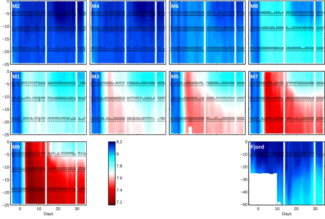
Figure S-4: Temporal development of pH (corrected to the total scale) in the mesocosms and the fjord as measured by a hand-operated CTD. Numbers at -5, -11 and -19 m depth denote daily averages representative for 0.3-5 m, 0.3-23 m and 15-23 m, respectively. For details on pH corrections applied see section 3.5.
10 15 20 25
30 0 I II III IV
a
1 2 3 4 5 6
b
0 0.1 0.2 0.3 c
0 5 10 15 20 25 30 35
0 0.2 0.4 0.6 0.8
Days
d
80 100 120
140 0 I II III IV
e
2 4 6 8 10 12 14
f
0 5 10 15 20 25 30 35
0 0.1 0.2 0.3 0.4
Days
g
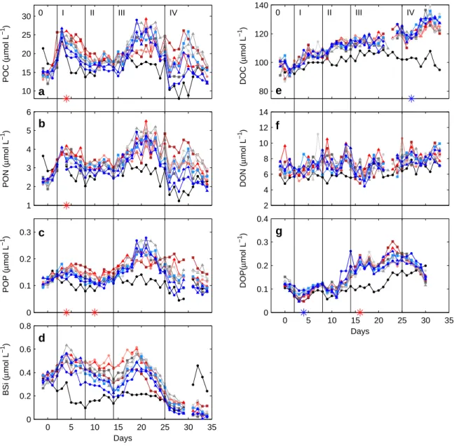
BSi (µmol L−1 )POP (µmol L−1 )PON (µmol L−1 )POC (µmol L−1 ) DOP(µmol L−1 )DON (µmol L−1 )DOC (µmol L−1 )
Figure S-5: Temporal dynamics of depth-integrated (0-23 m) POC (a), PON (b), POP (c), BSi (d), DOC (e), DON (f) and DOP (g) inside the fjord and the mesocosms. Note that concentrations for DOP have been smoothed by applying a three day running mean. Style and color coding follow that of Fig. 2.
0 0.2 0.4 0.6
a
Hapto (µmol C L−1 )
0 0.2 0.4 0.6
−1 Dino (µmol C L) NT b
0 0.2 0.4 0.6
c
Dino T (µmol C L−1 )
0 10 20 30
0 0.2 0.4 0.6
−1 Diatoms (µmol C L) d
Days
0 0.2 0.4 0.6
−1Chloro (µmol C L) e
0 0.5 1 1.5 2 2.5
−1Crypto (µmol C L) f
0 0.2 0.4 0.6
−1 Dino (µmol C L) HT g
0 10 20 30
0 0.5 1 1.5 2 2.5
−1 Total (µmol C L) autotroph h
Days
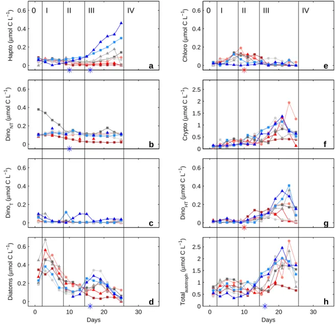
0 I II III IV 0 I II III IV
Figure S-6: Temporal dynamics of depth-integrated (0-23 m) organic carbon biomass of haptophytes (a), non-toxic dinoflagellates (b), toxic dinoflagellates (c), diatoms (d), chlorophytes (e), cryptophytes (f) and heterotrophic dinoflagellates (g) in side the fjord and the mesocosms, as determined by microscopy (see section 3.6 for details). The sum of the total autotrophic biomass is also shown (h). Style and color coding follow that of Fig. 2.