Exploring biogeochemical and ecological redundancy in phytoplankton communities in the global ocean

(1)

1196

|

wileyonlinelibrary.com/journal/gcb Glob Change Biol. 2021;27:1196–1213.

DOI: 10.1111/gcb.15493

P R I M A R Y R E S E A R C H A R T I C L E

Exploring biogeochemical and ecological redundancy in phytoplankton communities in the global ocean

Stephanie Dutkiewicz

^1,2

| Philip W. Boyd

³

| Ulf Riebesell

⁴

This is an open access article under the terms of the Creative Commons Attribution-NonCommercial License, which permits use, distribution and reproduction in any medium, provided the original work is properly cited and is not used for commercial purposes.

1Department of Earth, Atmospheric and Planetary Sciences, Massachusetts Institute of Technology, Cambridge, MA, USA

2Center for Global Change Science, Massachusetts Institute of Technology, Cambridge, MA, USA

3Institute for Marine and Antarctic Studies, University of Tasmania, Hobart, Tas., Australia

4GEOMAR Helmholtz Centre for Ocean Research Kiel, Kiel, Germany

Correspondence

Stephanie Dutkiewicz, Department of Earth, Atmospheric and Planetary Sciences, Massachusetts Institute of Technology, 54-1514 MIT, 77 Massachusetts Ave, Cambridge, MA 02139, USA.

Email: stephd@mit.edu Funding information

Simons Foundation, Grant/Award Number: 549931; Laureate, Grant/Award Number: FL160100131; NASA, Grant/

Award Number: 80NSSC17K0561

Abstract

Climate-change-induced alterations of oceanic conditions will lead to the ecological niches of some marine phytoplankton species disappearing, at least regionally. How will such losses affect the ecosystem and the coupled biogeochemical cycles? Here, we couch this question in terms of ecological redundancy (will other species be able to fill the ecological roles of the extinct species) and biogeochemical redundancy (can other species replace their biogeochemical roles). Prior laboratory and field studies point to a spectrum in the degree of redundancy. We use a global three-dimensional computer model with diverse planktonic communities to explore these questions further. The model includes 35 phytoplankton types that differ in size, biogeochemical function and trophic strategy. We run two series of experiments in which single phytoplankton types are either partially or fully eliminated. The niches of the targeted types were not completely reoccupied, often with a reduction in the transfer of matter from autotrophs to heterotrophs. Primary production was often decreased, but sometimes increased due to reduction in grazing pressure. Complex trophic interactions (such as a decrease in the stocks of a predator's grazer) led to unexpected reshuffling of the community structure. Alterations in resource utilization may cause impacts beyond the regions where the type went extinct. Our results suggest a lack of redundancy, especially in the ‘knock on’ effects on higher trophic levels. Redundancy appeared lowest for types on the edges of trait space (e.g. smallest) or with unique competitive strategies. Though highly idealized, our modelling findings suggest that the results from laboratory or field studies often do not adequately capture the ramifications of functional redundancy. The modelled, often counterintuitive, responses—

via complex food web interactions and bottom-up versus top-down controls—indicate that changes in planktonic community will be key determinants of future ocean global change ecology and biogeochemistry.

K E Y W O R D S

global change, marine biogeochemistry, marine ecology, phytoplankton, redundancy, trophic interactions

(2)

1 | INTRODUCTION

Climate change in terms of ocean warming, altered nutrient supply and acidification (Doney et al., 2012; Pörtner et al., 2014) could lead to significant re-arrangement of phytoplankton communities, with the potential for some species to become (at least regionally) extinct (e.g. Dutkiewicz, Morris, et al., 2015; Dutkiewicz et al., 2013; Litchman et al., 2015). Many modelling studies have targeted how phytoplankton communities will respond to changes in nutrient supply in a future ocean: changes in circulation and stratification will lead to lower supply of inorganic nutrients into the sunlight surface layer, favour- ing smaller species with higher nutrient affinity (Bopp et al., 2005;

Dutkiewicz et al., 2013; Dutkiewicz, Morris et al., 2015; Marinov et al., 2010). However, differing responses/sensitivity of phytoplankton species and strains to stressors other than nutrient supply (e.g.

direct impact of warming, ocean acidification) will likely also result in shifts in their relative competitiveness (Dutkiewicz, Morris, et al., 2015; Fu et al., 2014). Furthermore, it is an open question whether phytoplankton adaptation to ocean global change will occur fast enough (Collins et al., 2020; Ward et al., 2019), and whether a species will adapt in pace with their competitors, or with new invading competitors. Thus, such alteration in relative competitiveness (e.g. due to decreased growth rates, or higher susceptibility to grazing or viral infection) could result in some species losing their distinct niches and becoming extinct, at least regionally. This sequence of events raises questions regarding possible cascading effects within the planktonic community. Is there sufficient functional overlap in phytoplankton communities to buffer the loss of phytoplankton species due to ocean change? How will losses of phytoplankton species affect ecosystem functioning (termed here ecological redundancy) and the coupled oceanic biogeochemical cycles (termed here biogeochemical redundancy)? To address these questions, in this introduction, we first explore theoretical approaches to functional redundancy across disciplines including the terrestrial biosphere. Then we target evidence from laboratory and field studies to examine these concepts within oceanic settings. These ideas are then background for the suite of model experiments we discuss in the rest of the manuscript.

The topic of organismal function, in the context of diversity and hence redundancy, has been debated for several decades (Lavorel &

Garnier, 2002; Tilman, 1996), and has received considerable attention recently across a range of organisms, such as fish (Rice et al., 2013), corals (Bellwood et al., 2019), and birds and terrestrial mammals (Cooke et al., 2019). Conceptual advances, which have come largely from non-marine fields, are helpful to frame the issue of whether functional redundancy can offset the biogeochemical and ecological ramifications of ocean global change. Lavorel and Garnier (2002) con- flated concepts from Keddy (1992) and Chapin et al. (2000) to devise a multi-faceted structure—termed the response-effect-framework—

to probe the relationships between the influence of the environment (i.e. functional response) on diversity and ecosystem functioning (i.e.

ecosystem redundancy) of terrestrial plant communities. This concept has been discussed in the context of marine pelagic systems by Litchman et al. (2015), who pointed out the unique role of size as a

‘master trait’ in ocean systems where phytoplankton cell volume var- ies over nine orders of magnitude.

Another useful concept that informs functional redundancy is the relationship between multiple functions and biodiversity, termed ‘the multifunctionality context of biodiversity’ (Gamfeldt et al., 2008). This relationship dictates that there will be a decrease in redundancy (unless it is sustained by an increase in biodiversity) with an increase in the number of ecosystem functions and their degree of environmental control. Multifunctionality and its interactions with diversity have been investigated in microbial systems (Miki et al., 2014) and for soil fungal communities (Mori et al., 2015).

In contrast, aquatic systems have received less attention on this topic (Daam et al., 2019), with the major impasses thought to include incorporation of the many functions underpinned by ecosystems, the complexity associated with multiple trophic interactions, and the importance of spatial scales.

A major issue for the examination of functional redundancy in the open ocean is whether sufficient information is available on biodiversity, especially in relation to functionality. Daam et al. (2019) point out the potential utility of observational/experimental studies to better understand ecological function and biodiversity. Functional redundancy, in the context of ocean biogeochemistry, has previously been defined as the ‘ability of one microbial taxon to carry out a process [i.e. a function] at the same rate as another under the same environmental conditions’ (Allison & Martiny, 2008). In an oceanic context, ecological redundancy could similarly be defined as ‘ability of one taxon to fill the ecological niche of another’. However, such definitions might be too strict. The concept of redundancy is unlikely to be binary, there will more likely be a range or degree of redundancy: some species less redundant and some more. Similarly, it is unlikely that a single taxon will replace any extinct species. But could several taxa fulfil the biogeochemical function of a lost species? This leads to the question of how much will an ecosystem competition and trophic interactions be impacted by such losses?

In the ocean, we can probe and explore the concepts of functional redundancy (Tilman, 1996), functional responses (Lavorel &

Garnier, 2002), in both an ecological and biogeochemical context using illustrative examples from field observations, and laboratory and field environmental manipulation studies across different phytoplankton functional groups (Figure 1). The examples we found straddled high and low latitude provinces and nearshore and off- shore waters, and pointed to the likelihood of both high and low functional redundancy. For instance, in a manipulation study (Hoppe et al., 2017) using Arctic phytoplankton, there was a shift in diatom species composition in response to high CO₂ and irradiance conditions (partially mimicking year 2100 conditions), and both species were reported to have similar biogeochemical and ecological characteristics such as size and silicification (Figure 1b) and hence to have high redundancy. However, there are in fact considerable differences in the two species that might actually have led to low functional redundancy (c.f. Queguiner, 2013). In contrast, a high CO₂ mesocosm study in a high latitude fjord revealed a loss of competitive fitness of a key bloom-forming coccolithophore species with

(3)

multiple biogeochemical ramifications (Figure 1d; Riebesell et al., 2017). Other examples from the low latitude ocean point to different functional responses to environmental forcing (Figure 1a,c; Fu et al., 2014). Might replacement of Prochlorococcus with Synechococcus (or vice versa), two related picocyanobacteria, have minimal ecological and biogeochemical implications (Figure 1a), while a shift between large and small diazotrophs could have higher functional consequences on the fate of the new nitrogen (Figure 1c)?

These ‘thought experiments’ using published laboratory and field manipulation studies (Figure 1) are experimental ‘snapshots’ which leave many unknowns, and thus cannot permit full examination of potential feedbacks and ramifications within the marine system.

Thus, in this study to more broadly explore the concept of functional redundancy we use a global marine ecosystem model containing a complex planktonic community. The advantage of using a model is that idealized experiments can be undertaken to consider these concepts. Here, in particular, we consider the response of the model ocean to the loss, or partial loss, of single phytoplankton types and ask what consequences this will have on the plankton ecology (i.e.

influence on pelagic ecosystem at large) and biogeochemistry (i.e.

impact on rates with which energy and matter are transformed in the pelagic system). Though highly idealized, the model results en- able us to explore aspects of how the marine system might respond

to any species or group of species losing their niche or local competitiveness. The experiments provide us with insights into (the lack of) functional redundancy within the phytoplankton community.

2 | METHODS

2.1 | Model setup

The model follows from Dutkiewicz, Hickman, et al. (2015), Dutkiewicz et al. (2020) in terms of biogeochemistry, plankton interactions and transmission of light. Here we briefly provide an overview of the model and in particular its ecosystem structure. For more details, see supplemental material, and equations, values of pertinent parameters can be found in Dutkiewicz, Hickman, et al.

(2015), Dutkiewicz et al. (2020) and supplemental material.

The biogeochemical/ecosystem model resolves the cycling of carbon, phosphorus, nitrogen, silica, iron and oxygen through inorganic, living, dissolved and particulate organic phases. The biogeochemical and biological tracers are transported and mixed by the MIT general circulation model (MITgcm, Marshall et al., 1997) constrained to be consistent with altimetric and hydrographic observations (the ECCO-GODAE state estimates; Wunsch & Heimbach, 2007).

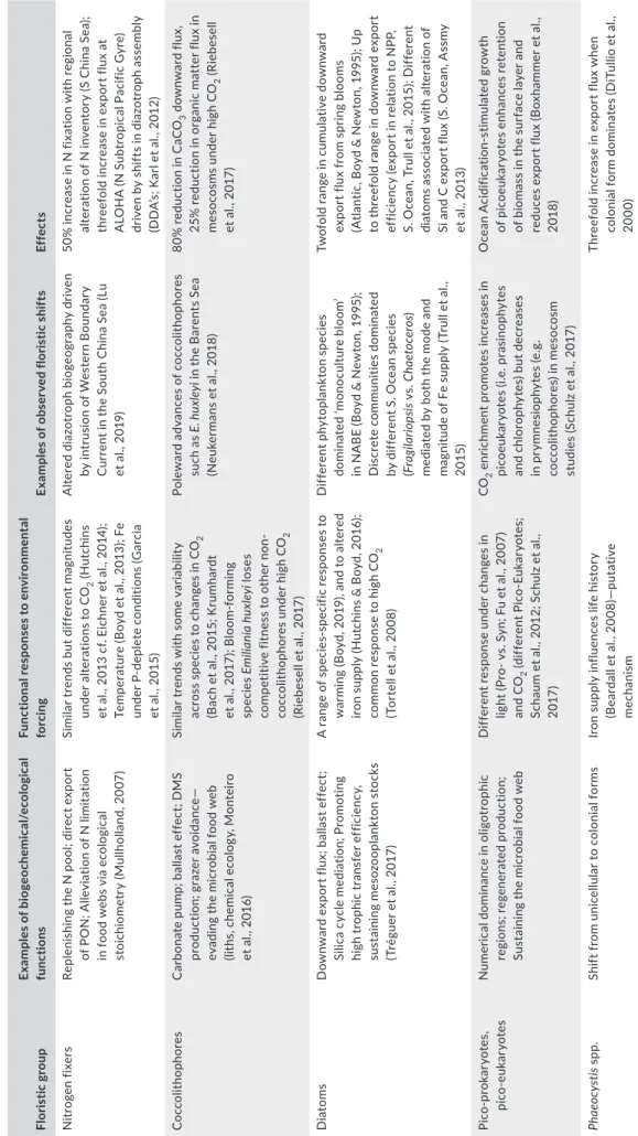
F I G U R E 1 Published examples for exploring redundancy. Schematics show functional response (left of each panel), and the wider future ramifications of such responses (right of each panel). These examples show differing degrees of functional redundancy, functional response to altered environmental forcing and the biogeochemical and/or ecological consequences. (a) Displays Synechococcus (blue symbols) and Prochlorococcus (green symbols), picocyanobacteriawhich are numerically dominant in the surface mixed layer and DCM (deep chlorophyll maximum) in oligotrophic regions. They have similar functions—but based on lab perturbation studies have different functional responses to future ocean conditions (Fu et al., 2007); (b) summarizes floristic shifts in Arctic pennate diatom communities between low and high CO₂ conditions (both under Iow and high light) that the authors (Hoppe et al., 2017) report are indicative of high functional redundancy, as depicted by the floristic and grazer schematics (though see Queguiner, 2013). Similar trends are recorded with Southern Ocean diatoms (Tortell et al., 2008); (c) focuses on diazotrophs in the low latitude ocean, which have similar functions (N fixation) but different biogeochemical and/or ecological consequences due to the different fates of the fixed N. Their different functional responses to warming (Fu et al., 2014) may result in altered partitioning of fixed N in a future ocean; (d) shows a shift in the bloom-forming abilities of coccolithophores (Emiliania huxleyi)—under high CO₂ conditions in a mesocosm study—along with altered biogeochemical functions (reduced downward export flux and DMS production; Riebesell et al., 2017). This shift in bloom-forming abilities under altered environmental conditions (high CO₂) in a mesocosm differs from the interpretation of time-series observations from the N Atlantic that showed an increase in coccolithophore abundances over 50 years; the authors linked this trend to increasing CO₂ concentrations (Rivero-Calle et al., 2015)

(4)

This three-dimensional configuration has coarse resolution (1° × 1°

horizontally) and 23 levels ranging from 10 m in the surface to 500 m at depth. At this horizontal resolution, the model does not capture mesoscale features such as eddies and sharp fronts.

We use a marine ecosystem that incorporates 35 phytoplankton types (Figure 2). These include several biogeochemical functional groups: diatoms (that utilize silicic acid), coccolithophores (that cal- cify), mixotrophs (that photosynthesize and graze on other plankton), nitrogen fixing cyanobacteria (diazotrophs) and pico-phytoplankton.

We resolve four size classes of pico-phytoplankton (from 0.6 to 2 µm equivalent spherical diameter, ESD), five size classes of coccolithophores and diazotrophs (from 3 to 15 µm ESD), 11 size classes of diatoms (3 to 155 µm ESD) and 10 of mixotrophic dinoflagellates (from 7 to 228 µm ESD).

Following the concept of size as a ‘master trait’ (Litchman et al., 2015; Ward et al., 2012), phytoplankton parameters influencing maximum growth rate, nutrient affinity and sinking are parameterized as a function of cell volume, though with distinct differences between functional groups as suggested by observations (see Buitenhuis et al., 2008; Dutkiewicz et al., 2020; Sommer et al., 2017). Following empirical evidence, mixotrophic dinoflagellates are assumed to have lower maximum photosynthetic growth rates than other phytoplankton of the same size (Tang, 1995).

To incorporate multiple trophic interactions, we resolve 16 size classes of zooplankton (from ESD 6.6 to 2,425 μm) that graze on plankton (phyto- or zoo-) 5–20 times smaller than themselves, but preferentially 10 times smaller (Hansen et al., 1997; Kiorboe, 2008;

Schartau et al., 2010). Mixotrophic dinoflagellates also graze on plankton in a similar fashion. Maximum grazing rate is a function of size (as in Dutkiewicz et al., 2020; following Hanson et al., 1997) with

mixotrophic dinoflagellates having a lower maximum grazing rates than other zooplankton of the same size (Jeong et al., 2010).

Almost all phytoplankton follow the allometric ‘rules’ as described above: growth, sinking and grazing pressure within any functional group are dictated by their size. The only ‘rule breaker’ captured in this model setup is the largest diazotroph (see Mulholland, 2007).

Growth and nutrient affinity are based on a single cell; however, since Trichodesmium exists in trichomes and most commonly in large colo- nies, we parameterize this diazotroph to be grazed much less heavily than other plankton the same size (see e.g. Bonnet et al., 2016; Hunt et al., 2016). We explore how the exact parameterization affects these results, see Supplemental text S3.2. Though potentially important for the concept of redundancy, we do not parameterize other ways to break the allometric rules, such as symbioses, multi-morphism, etc.

We will refer to each of the 35 phytoplankton as ‘types’ as they do not fit neatly into the definition of ‘species’. Though we can call the smallest type an analogue of Prochlorococcus, we note that we are combining many ecotypes into one category. And, for instance, our classification of the smallest diatom class encompasses many diatom species that are 3 μm ESD.

2.2 | Default simulation

We perform a ‘default’ simulation (EXP-0) for 20 years. The ecosystem quickly (within 2 years) reaches a quasi-steady state. Here, we show biomass of the plankton (Figure 2) and primary production and export flux, herbivory and nitrogen fixation rates (Figure 3) from the last 5 years of the simulation. The model captures the patterns of high and low productivity observed in the real ocean. The

F I G U R E 2 Model annual mean plankton biomass (mg C m⁻³) over the top 50 m of the model. Results for default experiment (EXP-0). Plankton are arranged by biogeochemical/

trophic functional group in columns.

Rows indicate the equivalent spherical diameter (ESD) in μm of the plankton, labelled on the left for phytoplankton (and mixotrophs) and on the right for zooplankton

(5)

distribution and abundances of size classes (Figure S1) and functional groups (Figure S2) also compare well to observations (e.g. Buitenhuis et al., 2013; Ward, 2015). Similar versions of this ecosystem model have been run with a variety of physical frameworks (e.g. Dutkiewicz et al., 2020; Kuhn et al., 2019; Sonnewald et al., 2020; Tréguer et al., 2017) and evaluated against several in situ and satellite products.

Additional evaluations of this exact default simulation are discussed in the supplemental material.

To explore the concept of redundancy, we conducted two series of sensitivity experiments. In one set, we instantaneously eliminate a single phytoplankton type and explore the ecological and biogeochemical consequences. In this series (‘Full Elimination’ Experiments), we are agnostic as to the driver of the extinction, loss of competitiveness could come from reduced ability to take up nutrients, decreased growth rates, higher susceptibility to grazing or viral infection among others. In these holistic experiments, we can examine the relative level of redundancy between all 35 model phytoplankton types. In the second series of experiments, we consider how various degrees of reduction in growth rate lead to partial or regional loss of single phytoplankton types. We refer to these as ‘Partial Elimination’ Experiments.

2.3 | Full Elimination Experimental Setup

Starting at the end of year 10 of the default experiment, we instantaneously and completely eliminate a single phytoplankton type (e.g.

the smallest type, an analogue of Prochlorococcus) and run the ex- periment out for another 10 years. To conserve matter, we take the biomass of the extinct phytoplankton type and add it to the detrital matter pool. A stable new community structure is reached within a couple of years and longer experiments (i.e. >10 years from the start of these sensitivity experiments) do not show substantially different results. Biogeochemical changes that affect the inventory of deep water nutrients would take several hundred to thousands of years to manifest and are beyond the scope of this study. We conduct 35 experiments where we eliminate each of the phytoplankton types individually. These experiments are labelled EXP-XY, where X represents which functional group (X = P,C,Z,T,M for pico, coc- colithophore, diazotroph, diatom and mixotrophic dinoflagellate, respectively), and Y which size class (Y = 1–11) within the functional group is eliminated. For example, the experiment where the smallest

pico-phytoplankton is eliminated is labelled EXP-P1, and for the second smallest diatoms being eliminated: EXP-T2.

2.4 | Partial Elimination Experimental Setup

In this set of experiments, we focus on three phytoplankton types:

Prochlorococcus-analogues, Trichodesmium-analogues and the small- est diatoms. For each of these types, we ran seven different sensitivity experiments where we instantaneously reduce the maximum growth rate of that type at the end of year 10 and ran the simu- lations for another 10 years. We decreased the maximum growth rate by different amounts for each of the seven experiments: from a 10% reduction to a 70% reduction. The reduced growth rate led to a decline in the globally integrated biomass of the targeted type (i.e.

‘partially eliminated’). As in the Full Elimination Experiments, a stable new community structure is reached within a couple of years.

2.5 | Diagnostics

Results shown in the remainder of the study consider the annual mean from the last year of each of the sensitivity experiments and compare them to the last year from the default simulation (EXP-0). To explore the ecological impacts of the loss of a phytoplankton type, we consider the changes in biomass of the remaining phytoplankton types relative to the default experiment (labelled EXP-0). To explore which types are replacing or being affected by the loss of the eliminated (or partially eliminated) type, we consider the changes to total global biomass. To explore how much of the ecosystem is affected, we calcu- late how many phytoplankton types have a significant change in each location. Here we assume ‘significant’ is a change in local biomass of any type to more than double or less than half of its biomass in EXP-0.

The values we chose (>50% decrease or >100% increase) are relatively arbitrary, but we conduct the same diagnostics with different values (>33% decrease or >50% increase; >10% decrease or >10% increase) and, though the numbers change, the patterns and insight do not.

To explore the biogeochemical impacts, we consider the local percentage difference of the depth integrated rates (primary production, grazing and nitrogen fixation) and carbon export through 100 m depth between each experiment and EXP-0.

F I G U R E 3 Annual mean default model biogeochemical rates. Depth integrate (a) primary production (g C m⁻² year⁻¹);

(b) export of carbon through 100 m (g C m⁻² year⁻¹); (c) herbivorous grazing rates (gC m⁻² year⁻¹); (d) nitrogen fixation rates (μmol N m⁻² day⁻¹)

(6)

2.6 | Caveats

This study was by design highly simplistic, but provides insights into potential consequences of losses of phytoplankton species in a future ocean. However, the results should be interpreted within the limitation of the model parameterizations. The highly restrictive grazing kernel (5-to-15:1 predator to prey ratio, and especially the 10:1 preference) and the simplistic parameterization of mixotrophy are two such parameterizations that should be kept in mind.

Additionally, we are considering ‘types’ of phytoplankton (e.g. a group of diatoms with ESD 3 µm) rather than ‘species’. Thus, the results we present below are more extreme than might occur in the real ocean when niches are lost in the future. In the following, we focus on and distinguish those results we believe are insightful, and add caveats where we consider that results are potentially compro- mised by model limitations.

3 | RESULTS

3.1 | Full elimination experiments

We show detailed results from four of the 35 experiments (EXP- P1, EXP-Z5, EXP-T1, EXP-M1), and otherwise summarize the other experiments. We describe the results for EXP-P1 in some detail to introduce the reader to the metrics employed.

3.1.1 | EXP-P1

In EXP-P1, the smallest type (model analogue of Prochlorococcus) is excluded from the system. The model results suggest that, as expected, the next smallest type (the model analogue of Synechococcus) increases in biomass (Figure 4b), replacing the small- est type, at least to some degree. However, there are other, potentially not as immediately intuitive, responses from other plankton.

We find that the 6.6 μm coccolithophore has an increase in biomass that almost matches the increase in Synechococcus globally.

This result is explained by links through the trophic levels: the loss of Prochlorococcus leads to a decrease in the smallest zooplankton (6.6 μm) which preferentially preyed on Prochlorococcus. This, in turn, leads to a reduction in the zooplankton class that is 10 times larger than the smallest zooplankton (i.e. because stocks of its prey were reduced). But this zooplankton also preyed on the 6.6 μm coccolithophore. With lower grazing pressure, this coccolithophore had an increase in biomass in some regions in the sensitivity experiment.

The model's parameterization of grazers preferentially targeting plankton 10 times smaller than themselves probably leads to this trophic-linked response being too strong relative to what might occur in the (more complex) real ocean. However, it has been docu- mented that there is some degree of size specific grazing in the real world (Hansen et al., 1997; Kiorboe, 2008; Schartau et al., 2010) as well as studies indicating that some grazers prefer specific prey (e.g. Prochlorococcus over other potential prey, Frais-Lopez et al.,

F I G U R E 4 Full Elimination Experiments: Global plankton biomass. (a) Annual mean globally integrated biomass (TgC) for each of the 51 plankton types in the default experiment (EXP-0). The plankton types are separated by colour of bar into function/trophic groups, and arranged within groups from smallest to largest in terms of ESD (μm). (b–e) Change in global plankton biomass (TgC) relative to default experiment (as seen in a) for four (of the 35) example experiments. Large cross indicates the extinct phytoplankton type. Panels indicate difference between default experiment and experiments where the eliminated type is (b) smallest phytoplankton (analogue of Prochlorococcus; EXP-P1), (c) largest diazotroph (the ‘rule breaker’, analogue of Trichodesmium; EXP-Z5), (d) smallest diatom (EXP-T1), (e) smallest mixotrophic dinoflagellates (EXP-M1). Positive values indicate an increase relative to the default. In (b–e) the y-axis is limited to +-25 TgC for clarity, where the changes are greater, the number is added to at the end of the bar

(7)

2009; Ribalet et al., 2015). We posit that this study indicates the complex trophic structures that could be altered by loss of any species/size class. In this experiment, it is not just these two phytoplankton types that are impacted by the loss of Prochlorococcus. We find that many other model phytoplankton types are substantially influenced (Figure 5, left column). Some types (e.g. Synechococcus and some size classes such as coccolithophores) have an increase in biomass (Figure 5, second row), but some types also have a decrease in biomass in some regions (Figure 5, bottom row). The demise of this smallest type leads to a substantial reconfiguration of the ecosystem, with some regions seeing substantial changes in as many as 12 (of the 35) phytoplankton types. Thus, from the terms of ecological redundancy (‘ability of one taxon to fill the ecological niche of another’), we can state that the model suggests that Prochlorococcus is not redundant.

In most regions where Prochlorococcus made up a substantial portion of the biomass (Figure 6, left column) there is a reduction in primary production. This suggests that the replacement types do not grow as well as Prochlorococcus in these regions of very low nutrient supply: they are not as well adapted to these conditions and their growth rates are subsequently lower. The local decreases in primary production can be as high as 20%. Though the responses in the regions where Prochlorococcus has a substantial biomass in EXP-0 are mostly negative for primary production, we find some regions just downstream (i.e. an adjacent region towards which the water flows) can have very slight positive responses (difficult to see with the colour bar in Figure 6). Some of the nutrients not efficiently consumed within the areas of reduced primary production are advected into downstream regions which then lead to an increase in primary production there. Thus, in terms of biogeochemical redundancy (‘ability of one microbial

taxon to carry out a process at the same rate as another’), the model results suggest that Prochlorococcus is also not redundant.

Primary production is reduced: no other taxon or combination of taxa can fully refill the functional role. Moreover, the impacts are not just local, but the functioning of downstream regions is also impacted.

This lack of biogeochemical redundancy is also seen in other rates. Export flux is greatly reduced in many regions where the primary production is reduced (Figure 6, second row). However, switching to larger species can lead to increased export efficiency, and even in some regions increased downward export flux, especially in the downstream regions where there is a slight increase in primary production. In the low biomass regions, a small change in primary productivity led to a larger response in the next trophic level seen by looking at the total herbivory rates (Figure 6, third row).

Another potentially surprising response is the large increase in nitrogen fixation rates in some regions (Figure 6, bottom row). In regions where the phytoplankton are nitrogen limited, slower con- sumption of iron and phosphate by the non-diazotroph replacement species (relative to Prochlorococcus) leads to additional excess of these nutrients (see e.g. Dutkiewicz et al., 2012; Ward et al., 2013) resulting in higher diazotroph biomass and higher nitrogen fixation.

This trend in nitrogen fixation generally occurred due to increase in larger diazotroph types (Figure 4b). This increase in nitrogen fixation can act to partially compensate for the decrease of primary production from the loss of Prochlorococcus.

We summarize these results of the ecological and biogeochemical responses in Figure 7. The first set of symbols in Figure 7a shows the maximum/median number of types significantly impacted by the loss of Prochlorococcus (as deduced from Figure 5, left column). We show total (black), as well as how many increase (red) and decrease

F I G U R E 5 Full Elimination Experiments: Ecological impacts—Phytoplankton types significantly impacted. (Top row) Total number of types

‘significantly’ affected between experiment and EXP-0; (second row) number of types whose biomass more than doubled in the sensitivity experiment; (third row) number of types whose biomass more than halved in the sensitivity experiment. Top row is the sum of second and third rows. Different values of cut-off (i.e. doubled/halved) were also considered (see Section 2): values change, but patterns and insight remained the same. Left column is experiment where smallest picophytoplankton (analogue of Prochlorococcus) is eliminated (EXP-P1);

second column for largest diazotroph (analogue of Trichodesmium), (EXP-Z5); third column for smallest diatom (EXP-T1); fourth column for smallest mixotrophic dinoflagellate (EXP-M1). White area is where the community was not impacted (mostly regions where the eliminated type was not in existence in the default experiment, see Figure 2)

(8)

(blue) their locally existing biomass. The median number of types/

species that increase is the same as decrease, though note these do not necessary occur in the same location (Figure 5). This leads to

some regional reshuffling of the communities. The biogeochemical results are summarized in the first set of bars in Figure 7b,c. The first green bar shows the range of local (i.e. in any model 1^o × 1^o F I G U R E 6 Full Elimination Experiments: Biogeochemical impacts relative to default. Colour shows percentage difference calculated as result from the sensitivity experiment minus EXP-0, divided by EXP-0 and multiplied by 100. (top row) Primary production; (second row) Export through 100 m; (third row) Total herbivorous grazing rate; (bottom row) Nitrogen fixation. Contours indicate where the lost type was >5% of the total phytoplankton biomass in EXP-0. Left column is experiment where smallest picophytoplankton (analogue of Prochlorococcus) is eliminated (EXP-P1); second column for largest diazotroph (analogue of Trichodesmium), (EXP-Z5); third column for smallest diatom (EXP-T1); fourth column for smallest mixotrophic dinoflagellate (EXP-M1)

F I G U R E 7 Full Elimination Experiments: Summary. Bars/symbols for each experiment where a single phytoplankton type was eliminated;

experiments separated by vertical dashed lines and arranged within functional groups from smallest to largest with number on x-axis showing the ESD of the eliminated type. Experiment designator (e.g. P1 etc., see Section 2) is also shown on x-axis. (a) Ecological impact, defined here as the number of phytoplankton types significantly impacted in the sensitivity experiment (see Figure 5, and caption); shown is the maximum number impacted at any location (top symbol) and the median number of types (lower symbol) in areas >1 (i.e. coloured areas in Figure 5a), red is the number with increasing biomass, blue for decreasing and black for total. (b, c) Biogeochemical impact (see Figure 6).

(b) Range of the local % change in primary production (green), export flux (red), herbivorous grazing rate (blue). When local values extend beyond the bounds of the y-axis, numbers are noted just inside of the graph. (c) % area of the ocean with more than 1% change (positively upward from centre line, and negatively down from centre line), same colour as in (b). For clarity of the figure, we do not show results for experiments where eliminated phytoplankton were larger than 32 μm, as these had more minor responses as they existed in less regions and lower biomass (see supplemental for caveat). See Figure S3 to see % area for area affected more than ±5% and >10% changes

(9)

grid cell) response in primary production in EXP-P1 (Figure 7b, from

−20% to +3%). A larger area of the ocean had decreased production than the area with increased (Figure 7c). The red bar indicates the range of local responses in export flux (Figure 7b, from −18% to +5%), with substantial parts of the ocean having an increase in export flux (Figure 7c). The blue bar indicates the range in local grazing responses (Figure 7b, −31% to +16%). This range is larger than for primary production, and a much larger area (>40%) has a decrease in grazing rate than had an increase (8%, Figure 7c). This indicates the trophic amplification. We do not show the change in local nitrogen fixation in the same way in this summary bar of Figure 7b as shifts in regions of where diazotrophy can exist lead to ±100% changes.

3.1.2 | Summary of other full elimination sensitivity experiments

The remaining sets of symbols/bars in Figure 7 summarizes the response from most of the rest of the 35 experiments. The largest diatoms and dinoflagellates only survived with very small biomass (see supplemental text), in the default model and thus, for clarity, results from the experiments that eliminate these types are not shown in Figure 7. In most experiments, there was substantial regional changes, both ecologically and biogeochemically. In general, similar number of phytoplankton types had decreases in biomass as increases in response to the loss of a single type (Figure 7a).

Biogeochemical responses ranged across both positive and negative in all experiments (Figure 7b). Some of the largest local changes occurred for the elimination of the smaller diatoms (Figure 7a,b). In terms of local changes to biogeochemical rates, the largest changes came from the largest diazotroph (EXP-Z5). The modelled mixotrophs had some of the smallest responses both ecologically and biogeochemically. Responses in export flux had smaller ranges locally than for primary production, suggesting that shifts in both phytoplankton and zooplankton size classes could compensate for changes in primary production. This trend could occur in particular when larger size classes dominated the replacement types in regions with reduced primary production (as seen in EXP-P1). In almost all experiments, there was a larger reduction in grazing (blue bars in Figure 7c) and the range of local response was amplified relative to primary production. To explore these differing biogeochemical responses in detail, and scrutinize the ecological consequences, we provide more details of the results from EXP-Z5, EXP-T1 and EXP- M1 (Figures 4–6).

EXP-Z5: One of the largest local responses in primary production (Figures 6 [second column] and 7b) occurs for the loss of the largest diazotroph (analogue of Trichodesmium). As mentioned earlier, this is the only type in the model that broke the allometric ‘rules’ in terms of grazing pressure: Given that Trichodesmium is usually found in large colonies and is thought to have few predators, we modelled the palatability of this phytoplankton type as being less than others. The reduced grazing pressure allowed this large diazotroph to expand is biogeographical range, and the amount of biomass it could

accumulate, more than in an experiment without this advantage. This concurs with suggestions based on observations (e.g. Mulholland, 2007; Turk-Kubo et al., 2018). In the sensitivity experiment where this type was eliminated (EXP-Z5), there were changes in the other four unicellular diazotroph biomasses (Figure 4c) suggesting these other types were trying to fill its niche; however, there were never- theless other significant shifts in community structure as seen in the Indian Ocean for instance (Figures 5 [second column] and 7a). Large regional biogeochemical responses occurred (Figure 6, second column), though they were limited in areal extent since the diazotrophs only exist in a limited region of the ocean (see Figure 2). Where the Trichodesmium-analogue was the only diazotroph that could survive, or where it was strongly the dominant type, (see Figure 2) there was a large reduction in nitrogen fixation. In most of these regions, there was also a reduction in primary production and export flux:

the nitrogen that the Trichodesimium-analogue fixed supported substantial productivity. However also notably, there are surrounding regions with an increase in nitrogen fixation and productivity with the loss of the Trichodesmium-analogue. Rearrangement of nutrient supply from the loss of this diazotroph type (in particular, the excess in iron and phosphate that was consumed by Trichodesmium) is now consumed elsewhere, spurring the increase in some of the other diazotrophs’ biomass. These shifts in biogeochemical rates led to other types (i.e. not only diazotrophs) being affected (i.e. Figure 7a shows that in some regions as many as 10 types were affected significantly).

In the model, the Trichodesmium-analogue biogeography, and the strong response to its elimination is a result of its reduced grazing pressure. We conducted an additional series of sensitivity experiments to test the robustness of the results to the specific method of parameterizing of this reduced grazing pressure and found our results qualitatively similar (see supplemental text S3.2; Figures S11 and S12).

EXP-T1: The largest re-arrangement of the ecosystem and largest biogeochemical response comes from the experiment where the smallest (fastest growing) diatom was removed (Figures 4d, 5 [third column], 6 [third column] and 7). In this experiment, there was a substantial increase in the biomass of the replacement types:

in this case, the second smallest diatom and a similar sized coccolithophore were the main types to respond (Figure 4d). However, there were many other types (e.g. larger diatoms, other coccolithophores) that had significant changes in biomass, both positive and negative (Figure 5). The growth rates of the replacement types are lower than for the smallest diatom (i.e. it is parameterized to have the fastest growth under nutrient replete conditions, see supplemental text). Even though the replacement types grow slower, primary production increases in some regions (Figure 6). This apparent incon- sistency is a consequence of concomitant even larger decrease in grazing pressure (Figure 6), allowing a larger phytoplankton standing stock (biomass) of the slower growing types. Grazing becomes more dominated by larger zooplankton types (Figure 4d) which are parameterized to have a lower maximum grazing rate (following Hansen et al., 1997). This larger standing stock of phytoplankton compen- sates for the lower growth rates such that some regions have an

(10)

increase in primary production and export flux. As with the two pre- vious experiments detailed here, there are compensatory responses in some regions (i.e. a decrease in productivity downstream) due to changes to the nutrient supply due to altered primary production and community structure.

EXP-M1: In the model, mixotrophic dinoflagellates are parameterized to photosynthesize and graze slower than similar sized specialists (as suggested by observations, Jeong et al., 2010; Tang, 1995). The modelled mixotrophs survived in regions where there was sufficient supply of both nutrients and prey. In EXP-M1, where the smallest mixotroph was removed, its niche was jointly filled by a similar sized phytoplankton (the 6.6 μm coccolithophore) and a 6.6 μm zooplankton, though also with Prochlorococcus (Figure 4e).

This trend is in contrast to most other experiments where the main replacement type was from within the same functional group as the extinct type (see Figure 4b–d). The replacement types in EXP-M1 were at least as efficient (or more) as the removed mixotroph type in either growth rate (in the case of the coccolithophore) or grazing (as in the zooplankton), thus due to this dual action the local responses were somewhat muted relative to other sensitivity experiments (Figures 5 and 6, 4th columns). There was also less impact on the rest of the ecosystem (Figure 5). We caution that the level of this muted response might be to some extent an artefact of the simplic- ity of how we parameterize these mixotrophic organisms. However, it does suggest that if a combination of replacement types (in this

case, a phytoplankton and a zooplankton) took over different roles of an extinct species, then there was potentially redundancy.

3.2 | Partial elimination sensitivity experiments

In the ‘Full Elimination’ Experiments, the explanation for the extinction of any phytoplankton type was not explored. Given that in all experiments there was a total loss of the selected phytoplankton type we could compare the experiments as done in Figure 7 to explore relative redundancy among the eliminated types. However, these experiments are highly artificial with respect to the immediate loss of phytoplankton types. In the real world, species losses are likely to be gradual (Pörtner et al., 2014). It is beyond the scope of this study to explore the temporal trajectory of extinctions and the gradual changes in ecological and biogeochemical consequences.

However, in this series of sensitivity experiments, we assess whether a partial loss of a phytoplankton type had significant ecological and biogeochemical impacts, and how these related to those from the full elimination experiments. We highlight only one mechanism for the loss of competitiveness leading to the lower biomass: reduction in maximum growth rate. We note that a more in-depth study (also outside the scope of this paper) would consider other reasons for loss of competitiveness, such as higher susceptibility to grazing or viral infection. We explore three cases: the partial elimination of

F I G U R E 8 Partial Elimination Experiments: Ecological Impacts. Change in annual mean globally integrated plankton biomass (Tg C) relative to default experiment (EXP-0, as seen in Figure 4a) where partially eliminated types’ global biomass was approximately half that in the default.

The amount reduction in maximum growth rate was different for the different types. Experiments where (a) smallest phytoplankton (analogue of Prochlorococcus) had growth rate reduced 60% (compare to Figure 4b), (b) largest diazotroph (the ‘rule breaker’, analogue of Trichodesmium) had growth rate reduced 20% (compare to Figure 4c) and (c) smallest diatom (EXP-T1) had growth rate reduced 20% (compare to Figure 4d).

The plankton types are separated by colour of bar into function/trophic groups, and arranged within groups from smallest to largest in terms of ESD (μm). Large cross indicates the partially extinct phytoplankton type, % number show the exact amount of the reduced biomass. Positive values indicate an increase relative to the default. The y-axis is limited to +-25 Tg C for clarity, where the changes are greater, the number is added to at the end of the bar. Similar results for full set of experiments are shown in Figures S5–S7

(11)

Prochlorococcus-analogue, Trichodesmium-analogue and the smallest diatoms.

Here, we show results where each of these types has its global integrated biomass reduced by about half (Figures 8 and 9) while all results from all experiments are shown in the Figures S4–S10 (additional text on these results is available in Supplemental S3.1).

The Prochlorococcus-analogue as the smallest autotroph is difficult to outcompeted in oligotrophic conditions. It required a 60% decrease in its growth rate before the global biomass was reduced to about 50% relative to EXP-0 (see values in Figure 8). It only required a 20% decrease in growth rate of the Trichodesmium-analogue, and the smallest diatoms to reach 50% of their original global biomass.

The phytoplankton types went locally extinct on the edges of their biogeographic domain (see bluest areas in Figure 9a–c). These were usually regions where their biomass was lower relative to the total community biomass originally. For instance, Prochlorococcus- analogue went locally extinct at higher latitudes and diatoms in the subtropical gyres. We found significant ecological and biogeochemical impacts at 50% reduction (Figures 8 and 9), and in fact even for lower reductions in biomass (Figures S5–S10). The replacement types, or those influenced through predator interaction, were vir- tually identical as for full elimination (EXP-P1, EXP-Z5 and EXP-1, compare Figure 8 to Figure 4b–d). However, not surprisingly, the magnitude of some of these altered biomasses were lower than in the Full Elimination Experiment, especially when the alteration of growth rates was less, but are never-the-less substantial even for modest changes in biomass (see Figures S7–S10).

The biogeochemical consequences could be more different than the ecological consequences between full and partial elimination, particularly for primary production (compare Figure 9d,f to Figure 6).

For instance, while primary production was largely reduced in EXP- P1 (Figure 6, top left panel) in the 50% partial elimination experiment

(Figure 9d), there are regions of increased primary production. This trend is seen even more when maximum growth rate had smaller reduction (see Figure S7). The explanation is similar to that for EXP-T1 described above: Strong reduction in grazing due to shifts to slower growing grazers allows a larger standing stock of phytoplankton.

This nonlinear result changes as the Procholococcus-analogues are progressively eliminated (see Figure S7).

Crucially, this series of experiments suggest that even a relatively small reduction in a species’ abundance (e.g. as might happen as it is slowly outcompeted in an environment) can lead to significant ecological and biogeochemical impacts.

4 | DISCUSSION

Our study uses a highly idealized set of numerical experiments to help us explore how loss of niches and relative competitiveness of some phytoplankton species in the future ocean might impact the ecology and biogeochemistry of the oceans. The model experiments undertaken in this study showcase that the ecological and biogeochemical responses are complex with potentially unexpected trophic interactions and feedbacks, as well as non-local impacts.

The model results suggest there is a range of redundancy, especially in terms of (relatively) unique life strategies and multifunctionality (sensu, Gamfeldt et al., 2008).

This model study was by design highly simplistic but does begin to address the impasses in the marine field raised by Daam et al.

(2019) regarding the complexity associated with multiple trophic interactions, and the importance of spatial scales. Thus, the simu- lations provide insights into potential consequences of the loss of species in a future ocean. However, we remind the reader of some important limitations of this study. The loss of types, or reduction F I G U R E 9 Partial Elimination Experiments: Biogeochemical impacts. (a–c) Percent decrease in partially eliminated types’ biomass relative to EXP-0, % number is the exact globally integrated biomass decrease. Percentage difference to EXP-0 in (d–f) primary production; (g–i) Total herbivorous grazing rate. Left column is experiment where smallest picophytoplankton (analogue of Prochlorococcus) growth rate is decreased by 60%; second column for largest diazotroph (analogue of Trichodesmium) growth rate is reduced 20%; third column for smallest diatom growth rate reduced 20%. Percentage change is calculated as result from the sensitivity experiment minus EXP-0, divided by EXP-0 and multiplied by 100. Compare to results from full elimination in Figure 6. Contours indicate where the biomass of the partially eliminated types was >5% of the total phytoplankton biomass in EXP-0. Similar results for full set of experiments are shown in Figures S8–S10

(12)

in growth, in each experiment was immediate and only tracked for a short time period (a decade). In the real world, extinctions will take years (or longer; Neukermans et al., 2018). Likely longer-term (many decades) shifts in nutrient supply will lead to additional, more distant, downstream responses that are not captured in our study.

Additional caveats are as follows: the highly restrictive grazing kernel potentially leads to over-simplified trophic interactions; the sim- plicity in the parameterization of mixotrophy, and colony formation;

and that the model, though more complex than most, still only encompasses a small amount of the actual large diversity in the real world. The model does not incorporate evolutionary adaptation, intraspecific diversity and trait plasticity (e.g. Henn et al., 2018) which could substantially alter the risk of species to become extinct in the first place. However, if some species are better able to adapt to a changing environment, this could also lead to the extinction of other less adaptable species.

None of the individual experiments should be considered as a prediction of ecological or biogeochemical status of the future oceans. Moreover, extrapolating these results to any specific species in the real ocean is unwise. Instead, the results should be understood as providing insight into the relative redundancy to the ocean ecosystems and productivity, and processes and feedbacks that might otherwise not be expected from, or which could be tested within, laboratory and field experiments.

4.1 | Changes in functional responses

Numerous laboratory studies have suggested a variety of responses of different species to changes to the environment predicted by the end of this century: warming, acidification, alteration of the under- water light fields, as well as changes in nutrient supplies. We provide some examples in Table 1, third column. For instance, though most diazotrophs (unicellullar and colonies) had increased growth rates under high CO₂ conditions (Hutchins et al., 2013; Walworth et al., 2016), some species (unicellular) had larger responses than others.

This could lead to reduced fitness in the colonial species (akin to the Trichodesmium-analogue in the model) relative to others. Reduction in fitness of some species relative to others outside their functional group has also been seen in mesocosm experiments targeting coccolithophores (Riebesell et al., 2017). Such responses will likely lead to the reduction or termination of some species niches with subse- quent shifts in local planktonic community structure.

4.2 | Effects of shifts in community structure

Ocean acidification experiments in the field suggest shifts in phytoplankton community composition, succession and productivity (Bach et al., 2016), thereby increasing the transfer to higher trophic levels (Sswat et al., 2018), prolonging the retention of biomass in the surface layer and reducing export flux of C, N and P (Boxhammer et al., 2018). The illustrative examples from

experimental manipulation studies of shifts in community structure (e.g. Figure 1) in some cases have parallels in the ocean. For example, there was widespread evidence across a range of oceanic provinces, including the Bering Sea (Tyrrell & Merico, 2004), North East Atlantic (Rivero-Calle et al., 2015) and South China Sea (Lu et al., 2019) that substitution of one phytoplankton type for another resulted in altered biogeochemical and ecological signatures (Table 1). For instance, shifts in diazotroph populations driven by intrusions of a Western boundary current in the South China Sea led to a 50% increase in nitrogen fixation (Lu et al., 2019). In other examples, shifts in the dominant species during the diatom spring bloom in the North East Atlantic between years resulted in a twofold enhanced export flux to depth when a larger sized species was prevalent (Table 1). Other floristics shifts within diatom (in the Southern Ocean, Assmy et al., 2013) or diazotroph (to diatom- diazotroph assemblages in the North Subtropical Pacific Gyre, Karl et al., 2012) resulted in altered biogeochemical signatures of downward export flux (Table 1).

4.3 | Interlinked ecological and

biogeochemical redundancy

How much of the ecological and the biogeochemical change with the loss of a species can be couched in terms of the degree of redundancy? Here we have explored two, but explicitly intertwined, concepts of redundancy. By ecological redundancy, we contemplated how the loss of a phytoplankton type impacted the rest of the pelagic ecosystem. By biogeochemical redundancy, we asked if other type(s) could fulfil the biogeochemical functional role, such as primary production, as efficiently as a lost type. The answers to these two redundancy questions were however strongly dependent on each other. For instance, replacement type(s) did not transfer matter to higher trophic levels (as defined here as a biogeochemical impact) as efficiently as the lost species, with consequences for the grazing pressure on the phytoplankton, and hence impacting the community structure (ecological impact). For ease in the discussion, in this manuscript, we separate the two concepts, but this interlinking of the two concepts should be kept in mind.

4.4 | A range of ecological redundancy

Main replacements for the partial or full eliminated types are plankton that are next best suited to the environment (e.g. Synechococcus re- placing Prochlorococcus, or the next smallest diatom when the smallest diatom was eliminated), and are in general of the same functional group as the eliminated type. These responses echo the insight suggested by the laboratory experiments showcased in Figure 1. However, the model results suggest trophic interactions allowed for other less intuitive ecological responses. Impacts on the grazers with the reduction or loss of their preferred prey could lead to higher trophic responses, that, in turn, will lead to additional restructuring in the phytoplankton

(13)

TABLE 1 Illustrative examples from ocean field observations, and laboratory and field environmental manipulation studies. We show examples of several different floristic groups and highlight their biogeochemical and ecological functions. We synthesize (third column) some of the observed responses to environmental change that might lead to alterations or disappearance of their regional niches, (fourth column) some observed shifts in communities with alterations in environment, and (fifth column) the potential biogeochemical or ecological effects of such shifts Floristic groupExamples of biogeochemical/ecological functionsFunctional responses to environmental forcingExamples of observed floristic shiftsEffects Nitrogen fixersReplenishing the N pool; direct export of PON; Alleviation of N limitation in food webs via ecological stoichiometry (Mullholland, 2007) Similar trends but different magnitudes under alterations to CO2 (Hutchins et al., 2013 cf. Eichner et al., 2014); Temperature (Boyd et al., 2013); Fe under P-deplete conditions (Garcia et al., 2015) Altered diazotroph biogeography driven by intrusion of Western Boundary Current in the South China Sea (Lu et al., 2019)

50% increase in N fixation with regional alteration of N inventory (S China Sea); threefold increase in export flux at ALOHA (N Subtropical Pacific Gyre) driven by shifts in diazotroph assembly (DDA’s; Karl et al., 2012) CoccolithophoresCarbonate pump; ballast effect; DMS production; grazer avoidance— evading the microbial food web (liths, chemical ecology, Monteiro et al., 2016)

Similar trends with some variability across species to changes in CO2 (Bach et al., 2015; Krumhardt et al., 2017); Bloom-forming speciesEmiliania huxleyi loses competitive fitness to other non- coccolithophores under high CO2 (Riebesell et al., 2017) Poleward advances of coccolithophores such as E. huxleyi in the Barents Sea (Neukermans et al., 2018)

80% reduction in CaCO3 downward flux, 25% reduction in organic matter flux in mesocosms under high CO2 (Riebesell et al., 2017) DiatomsDownward export flux; ballast effect; Silica cycle mediation; Promoting high trophic transfer efficiency, sustaining mesozooplankton stocks (Tréguer et al., 2017)

A range of species-specific responses to warming (Boyd, 2019), and to altered iron supply (Hutchins & Boyd, 2016); common response to high CO2 (Tortell et al., 2008)

Different phytoplankton species dominated ‘monoculture bloom’ in NABE (Boyd & Newton, 1995); Discrete communities dominated by different S. Ocean species (Fragilariopsis vs. Chaetoceros) mediated by both the mode and magnitude of Fe supply (Trull et al., 2015)

Twofold range in cumulative downward export flux from spring blooms (Atlantic, Boyd & Newton, 1995); Up to threefold range in downward export efficiency (export in relation to NPP, S. Ocean, Trull et al., 2015); Different diatoms associated with alteration of Si and C export flux (S. Ocean, Assmy et al., 2013) Pico-prokaryotes, pico-eukaryotesNumerical dominance in oligotrophic regions; regenerated production; Sustaining the microbial food web

Different response under changes in light (Pro- vs. Syn; Fu et al., 2007) and CO2 (different Pico-Eukaryotes; Schaum et al., 2012; Schulz et al., 2017) CO2 enrichment promotes increases in picoeukaryotes (i.e. prasinophytes and chlorophytes) but decreases in prymnesiophytes (e.g. coccolithophores) in mesocosm studies (Schulz et al., 2017)

Ocean Acidification-stimulated growth of picoeukaryotes enhances retention of biomass in the surface layer and reduces export flux (Boxhammer et al., 2018) Phaeocystis spp.Shift from unicellular to colonial formsIron supply influences life history (Beardall et al., 2008)—putative mechanism Threefold increase in export flux when colonial form dominates (DiTullio et al., 2000)

(14)

communities (‘ripples’ through the food chain). This reduction in redundancy due to multiple trophic level effects concurs with the ecosystem multi-functionality concept of Gamfeldt et al. (2008).

Redistribution of nutrients due to shifts in biogeochemistry (discussed more below) also led to ecological impacts. For instance, another unexpected result was the increase in diazotrophs with the elimination of their competitor species such as picophytoplankton that freed up limiting resources. This again suggests the lower redundancy with multiple functioning ecosystems.

The model suggests that types with more complex trophic link- ages and especially those that dominate in highly productive regions supporting longer food chains (e.g. small diatoms) are less ecological redundant. Loss of such types will lead to substantial ripples up and back down the trophic chains. Types which had similar sized replacements (e.g. mixotrophs) appeared more redundant, though this result may be overstated because of the strong size-based parameterization of the grazing. Never-the-less, this result provides a unique and not necessarily intuitive insight into how multi-functionality at the species level might fit into the functionality/redundancy debate (e.g.

Gamfeldt et al., 2008).

4.5 | A range in degree of

biogeochemical redundancy

The model suggests that biogeochemical redundancy may also be lower for types (species) that are on the edges of trait spaces, for instance being the smallest or types that have unique strategies (e.g. Trichodesmium). Other phytoplankton with unique strategies, such as chain and colony formation (see e.g. Abada & Segev, 2018;

Beardall et al., 2008) and bi-morphism (e.g. Phaeocystis, not modelled here) are also likely to have low redundancy. It is probable that in the real ocean there are many more species that will have filled specific niches with other unique strategies and we might anticipate there being significant non-redundancy. Though clearly more research on this question is warranted.

The model results suggest that replacement types (at least without strong adaptation) will not grow as well in the same environment, leading to substantial biogeochemical responses. In the model, this manifested as a strong decrease in transfer to higher trophic levels, a trophic amplification. But the response for primary production was more varied depending on the nonlinear interactions between decreased predation and slower growth rates.

This complex bottom-up versus top-down response could shift as species were slowly eliminated (as seen in the partial elimination experiments).

The model only captures ‘groups’ (here called ‘types’) of phytoplankton (e.g. 3 μm ESD diatoms), with each group differing substantially from another in terms of nutrient requirements, nutrient uptake affinity and types of grazers. More ‘fine-grained’ shifts in species that may be more similar might have less impact. In the example of the Arctic diatom species shifts (Figure 1b, Hoppe et al., 2017), the authors interpreted their results as having little

biogeochemical change (i.e. high redundancy). However, another interpretation of this observed floristic shift (using broad categories employed by Queguiner, 2013) is that it could result in changes to both trophic transfer and export flux (i.e. influencing ecological and biogeochemical redundancy). Thus, we caution that even what may appear to be a minor difference in species could be amplified, caus- ing long-term effects in both ecology and biogeochemistry. There are also examples of even finer-grained intraspecific diversity in diatoms (e.g. Anderson & Rynearson, 2020; Rynearson et al., 2020) and in Prochlorococcus (e.g. Kashtan et al., 2014), differentiated often by temperature and light requirements. Understanding how intraspecific differences impact functional redundancy would be an inter- esting future study.

The biogeochemical impact of removing diazotrophs extended further than just changes in rates of nitrogen fixation but also impacted primary production, and in turn export flux and grazing rates.

This knock-on effect has a larger impact on carbon export flux than the anticipated (and modelled) lower export of diazotroph carbon with the removal of the Trichodesmium-analogue as anticipated from Figure 1c. So, although the ‘thought experiment’ gained from laboratory studies (Figure 1c) was correct, it missed the much larger impacts that were captured by feedbacks found in the model. But changes in diazotrophy could also occur due to elimination of their competitors (smaller phytoplankton). This resulted in local increases in nitrogen fixation allowing for compensatory supply of fixed nitrogen to the system in these experiments. These cross-functional/

trophic group feedbacks would also not a priori be anticipated from examination of laboratory and field experiments.

4.6 | Remote impacts

A potentially surprising result not anticipated from the field and laboratory examples was how many impacts were found beyond the area where the eliminated types had been major components of the ecosystem. In many experiments, there were regions with opposite responses in biogeochemical rates just downstream of the regions where the eliminated types had a larger population (Figure 6).

Subtle changes in nutrient supplies to these downstream regions in response to ecological/biogeochemical changes upstream led to this opposite response in productivity. In the experiments where the Trichodesmium-analogue was eliminated (EXP-Z5) we found that lower nutrient uptake in regions where this type had dominated the diazotroph biomass led to higher nitrogen fixation downstream, impacting primary production, and, in turn, export and grazing rates.

4.7 | Implications to climate change

Many model studies have examined shifts in communities from pro- jected reduction of nutrient supplies, specifically to favour smaller phytoplankton over larger types such as diatoms (e.g. Bopp et al., 2005; Dutkiewicz et al., 2013; Marinov et al., 2010). Modelling studies