Evaluation of the transport matrix method for simulation of ocean biogeochemical tracers

(1)

Evaluation of the transport matrix method for simulation of ocean biogeochemical tracers

Karin F. Kvale¹, Samar Khatiwala², Heiner Dietze¹, Iris Kriest¹, and Andreas Oschlies¹

1GEOMAR Helmholtz-Zentrum für Ozeanforschung Kiel, Düsternbrooker Weg 20, 24105 Kiel, Germany

2Department of Earth Sciences, University of Oxford, South Parks Road, Oxford OX1 3AN, UK Correspondence to:Karin F. Kvale (kkvale@geomar.de)

Received: 2 February 2017 – Discussion started: 6 February 2017

Revised: 3 May 2017 – Accepted: 23 May 2017 – Published: 29 June 2017

Abstract. Conventional integration of Earth system and ocean models can accrue considerable computational ex- penses, particularly for marine biogeochemical applications.

“Offline” numerical schemes in which only the biogeochemical tracers are time stepped and transported using a pre- computed circulation field can substantially reduce the bur- den and are thus an attractive alternative. One such scheme is the “transport matrix method” (TMM), which represents tracer transport as a sequence of sparse matrix–vector products that can be performed efficiently on distributed-memory computers. While the TMM has been used for a variety of geochemical and biogeochemical studies, to date the resulting solutions have not been comprehensively assessed against their “online” counterparts. Here, we present a detailed comparison of the two. It is based on simulations of the state-of-the-art biogeochemical sub-model embedded within the widely used coarse-resolution University of Vic- toria Earth System Climate Model (UVic ESCM). The default, non-linear advection scheme was first replaced with a linear, third-order upwind-biased advection scheme to sat- isfy the linearity requirement of the TMM. Transport matrices were extracted from an equilibrium run of the physical model and subsequently used to integrate the biogeochemical model offline to equilibrium. The identical biogeochemical model was also run online. Our simulations show that offline integration introduces some bias to biogeochemical quantities through the omission of the polar filtering used in UVic ESCM and in the offline application of time-dependent forcing fields, with high latitudes showing the largest differences with respect to the online model. Differences in other regions and in the seasonality of nutrients and phytoplankton distributions are found to be relatively minor, giving confi-

dence that the TMM is a reliable tool for offline integration of complex biogeochemical models. Moreover, while UVic ESCM is a serial code, the TMM can be run on a parallel machine with no change to the underlying biogeochemical code, thus providing orders of magnitude speed-up over the online model.

1 Introduction

The transport matrix method (TMM) (Khatiwala et al., 2005;

Khatiwala, 2007) is a numerical scheme for efficient simulation of ocean biological and chemical tracers. It is based on the idea that the advective–diffusive transport of a passive tracer is a linear operator, which, when spatially discretized, can be generically represented as a sparse matrix.

Time stepping of such tracers is thus reduced to a sequence of sparse matrix–vector multiplications, operations that can be carried out efficiently on modern, distributed-memory computers. While conventional ocean general circulation models (GCMs) do not typically represent transport in this manner, for many GCMs is it is possible to extract the corresponding matrix representation of the ocean’s tracer transport scheme, including sub-grid-scale parameterizations, by

“probing” it with patterns of 1’s and 0’s (Khatiwala et al., 2005). The transport matrix approach is also amenable to di- rect computation of equilibrium solutions, including period- ically (seasonally) repeating ones (Khatiwala, 2008). This is especially useful for “spin-up” of complex biogeochemical models, which requires several thousand year-long integrations.

(2)

2426 K. F. Kvale et al.: Online–offline comparison The TMM has been applied to a wide range of problems,

including simulating anthropogenic carbon uptake and radiocarbon by the ocean (Graven et al., 2012), simulating noble gases to improve the parameterization of air–sea gas transfer (Nicholson et al., 2011; Liang et al., 2013) and investigate ocean ventilation (Nicholson et al., 2016), studying ocean proxy (Siberlin and Wunsch, 2011) and radiocarbon (Koeve et al., 2015) timescales, investigating the mechanisms con- trolling nutrient ratios (Weber and Deutsch, 2010), modeling the cycling of particle reactive geochemical tracers (Jones et al., 2008; Siddall et al., 2008; Vance et al., 2017), estimating respiration in the ocean from oxygen utilization rates (Duteil et al., 2013; Koeve and Kähler, 2016), demonstrating the utility of atmospheric potential oxygen measurements to constrain ocean heat transport (Resplandy et al., 2016), modeling the ocean’s CaCO3 (Koeve et al., 2014) and nitrogen (Kriest and Oschlies, 2015) cycles; studying the impact of the Southern Ocean on global ocean oxygen (Keller et al., 2016), estimating the flux of organic matter (Wilson et al., 2015), and biogeochemical parameter sensitivity (Khatiwala, 2007;

Kriest et al., 2010, 2012) and optimization (Priess et al., 2013b, a; Kriest et al., 2017).

Despite these varied applications, a comprehensive evaluation of the TMM viz a vis results produced by the corresponding online model has not yet appeared in the published literature. Khatiwala et al. (2005) and Khatiwala (2007) provided a limited comparison between online and offline TMM simulations of a simple passive tracer and biogeochemical model using transport matrices extracted from the MITgcm (Marshall et al., 1997). For problems that use information gleaned from offline simulations to inform online simulations it is especially important that the offline simulations faithfully reproduce the online ones. Here, we provide the first such comprehensive assessment of the TMM based on version 2.9 of the University of Victoria Earth System Cli- mate Model (UVic ESCM Weaver et al., 2001; Eby et al., 2009), a coarse-resolution (1.8^◦×3.6^◦×19 ocean depth layers) ocean–atmosphere–biosphere–cryosphere–geosphere model. The marine nutrients–phytoplankton–zooplankton–

detritus (NPZD) biogeochemistry has increased in complexity since Eby et al. (2009), with the addition of iron limitation and revisions to zooplankton grazing (Keller et al., 2012), and subsequent minor updates. The NPZD model contains two phytoplankton types (a general type and diazotrophs) and a single zooplankton type, dissolved inorganic carbon (DIC), alkalinity, nitrate, phosphate (the base unit), and oxygen. Iron limitation is prescribed using a seasonally varying, three-dimensional (3-D) iron concentration field. Full model details can be found in Keller et al. (2012) and associated references. We describe the procedure to extract TMs (transport matrices) from the UVic ESCM ocean model and couple the biogeochemical model to the TMM framework. An equilibrium simulation of the biogeochemical model with the TMM is then compared with a conventional online simulation. We

discuss some of the compromises needed and their impact on the offline simulations.

2 Methods

2.1 Transport matrix extraction in UVic ESCM The TMM relies on the fact that the underlying partial differ- ential equation for transport of a passive tracer is linear with respect to advection and diffusion. If the discrete (numerical) implementation is also linear, the tracer time-stepping equation can be generally written in matrix form as (Khatiwala, 2007)

cⁿ⁺¹=A_i(A_ecⁿ+qⁿ), (1) wherenis the time step;cis a vector of tracer concentrations (the 3-D model grid mapped onto a vector);A_e is the “explicit” transport matrix representing horizontal advection–

diffusion (and, commonly, vertical advection) that is generally time stepped using an explicit, forward-in-time scheme;

A_iis the “implicit” transport matrix representing vertical diffusion (and, less commonly, vertical advection) that is typically time stepped using an implicit method; andqis a vector representing the sources and sinks of the tracer. Note thatA_i can be thought of as the inverse of the tridiagonal matrix arising in the implicit solution of the diffusion equation.

The procedure for extracting the TMs is described in de- tail in Khatiwala (2007). In essence it involves (1) initializ- ing the tracer field at the start of each time step with a “1” at a single grid point and “0” everywhere else; (2) computing the explicit tracer tendency, which in effect gives the corresponding column of the explicit matrix A_e; (3) resetting the tracer field to its initial pattern; and (4) applying implicit vertical diffusion, the result of which is the corresponding column ofA_i. The TMs are generally averaged over a number of time steps to give a time–mean matrix representation of the transport. In practice, the extraction can be consider- ably sped up by noting that many columns of the TMs are

“structurally independent” since tracer spreads only a finite (known) distance in a single time step. Multiple columns of Ae andAican thus be simultaneously computed by a judi- cious choice of the pattern of 1’s and 0’s. Such an optimal set of “basis functions” can be computed by combining knowl- edge of the model bathymetry and stencil of the advection–

diffusion scheme with graph coloring methods (Curtis et al., 1974; Coleman and Moré, 1983).

It is quite straightforward to implement the above procedure in an ocean model with only minor modifications to the code, and we have done so with UVic ESCM. How- ever, in practice a number of complications can arise. For example, ocean models sometimes use a non-linear advection scheme so as to avoid over- and undershoots arising from sharp gradients in the tracer field. In fact, UVic ESCM uses such a scheme, “flux-corrected transport” (FCT; Weaver

(3)

and Eby, 1997), by default. To reconcile this with the linearity requirement of the TMM, we instead use a third-order, upwind-biased scheme (Holland et al., 1998; Griffies et al., 2008) (hereafter “UW3”) that significantly reduces potential over/undershoots but is also much less diffusive than conventional first-order upwind. This scheme has already been implemented in UVic ESCM, but switching it on caused the strength of the meridional overturning circulation (MOC) in the model to decrease significantly. To obtain a MOC strength consistent with observations, we increased the vertical diffusion coefficient from 0.15 to 0.43 cm²s⁻¹. However, it is important to note that other parameters in the model, such as the atmospheric moisture diffusivity field, also have an impact on ocean circulation. These parameters were tuned for the FCT scheme but were left unchanged when switching to the UW3 scheme.

A second complication is from the time-stepping scheme, which in UVic ESCM is leapfrog. The explicit horizontal advection and diffusion terms are also sometimes stag- gered with respect to each other for stability. Both require storing the tracer field at odd and even time steps. While this can be replicated offline, in order to use a common scheme for all ocean models from which TMs have been extracted (e.g. MITgcm variously uses Adams–Bashforth, di- rect space–time discretization and other schemes), we com- bine horizontal advection and diffusion into a single explicit transport matrix, Ae, which is time stepped with a simple, forward Euler method. Specifically, to extract the explicit matrix, we only store the (passive) tracer field at the current time step. This field, which is reset to a pattern of 1’s and 0’s at the beginning of each time step, is then stepped forward by UVic ESCM like any other tracer. The change in the tracer field divided by the time step is the explicit tendency matrix.

With this procedure, which does not require changes to the underlying code, the usual leapfrog scheme is side stepped.

Lastly, UVic ESCM applies Fourier filtering in the zonal direction at high latitudes to remove grid-scale noise. The efficiency of the TMM arises from the fact that the discretized advection–diffusion operator has a limited stencil, i.e. only couples nearby points, giving rise to a sparse matrix. Fourier filtering on the other hand couples all points in the zonal direction, greatly reducing the sparsity of the transport matrix and hence the computational efficiency of the sparse matrix–

vector products at the heart of the TMM. While the cost of a sparse matrix–vector product is implementation- and hardware-dependent and non-trivial to analyze (e.g. Gropp et al., 2000), it roughly scales with the number of non-zero elements per row. With a third-order upwind scheme, there are a maximum of 5×5×5=125 non-zero elements per row.

With Fourier filtering that becomesnx×5×5, wherenxis the number of zonal grid points. In UVic ESCMnx=100, implying that the TMM would be roughlynx/5=20 times slower with Fourier filtering turned on. We therefore turn off polar filtering for the passive tracers used to extract the TMs.

The numerical treatment of temperature and salinity by the model is not altered.

The neglect of polar filtering and staggering of advection and diffusion terms necessitates using, for stability, a slightly smaller time step in offline simulations with the TMM compared with the online model. In the latter, the default time step for ocean dynamics and tracer transport is 1.25 days, a choice dictated by the need to synchronize the ocean model with the atmospheric one (which takes two time steps per ocean time step). (The biogeochemical terms in UVic ESCM are time stepped internally within the biogeochemical mod- ule using a much smaller time step such that there are three biogeochemical steps per ocean step.) No change was made to this during extraction of the TMs; i.e. the model physics and active tracers were integrated using the default time step.

Since the explicit TM is extracted as a tendency, the time step for offline explicit advection–diffusion can be subsequently set to any desired value. However, the implicit TM has a time step embedded within it. By default it would also be 1.25 days, but embedding a different time step is quite straightforward: during extraction of the implicit TM, we simply pass the desired time step as an argument to the sub- routine that solves for implicit diffusion. We have found an offline time step of 8 h (28 800 s) to be a good compromise between stability and accuracy. It is also very similar to the biogeochemical time step of the online model (27 000 s).

Using the linear UW3 advection scheme, the coupled physical–biogeochemical model was spun-up to equilibrium for 13 000 years with a fixed, pre-industrial atmospheric CO2

concentration of 277.4 ppm. The model was run for 1 additional year with the transport matrix extraction switched on.

During this run, explicit and implicit TMs were computed at each time step, and accumulated over the course of a month before being averaged and written out. These monthly mean TMs were subsequently used for the offline simulations. For comparison, we also carried out a similar spin-up of the physical and biogeochemical model using the default FCT advection scheme (see Appendix A).

2.2 Interfacing the UVic ESCM biogeochemical model to the TMM

Once the TMs have been extracted, biogeochemical tracers can be simulated offline via Eq. (1) using any convenient software. However, to facilitate use of the TMM for global simulations of complex biogeochemical models, Eq. (1) has been implemented using the open-source PETSc scientific library from Argonne National Laboratories (Balay et al., 2003). PETSc is a suite of data structures and routines de- veloped for large-scale linear and non-linear problems. In particular, it provides state-of-the-art, distributed-memory routines for operating on vectors and sparse matrices. The TMM driver code implementing Eq. (1) is freely available from https://github.com/samarkhatiwala/tmm. The code can be run without modification on most computers, serial or par-

(4)

2428 K. F. Kvale et al.: Online–offline comparison

(a) (b) (c)

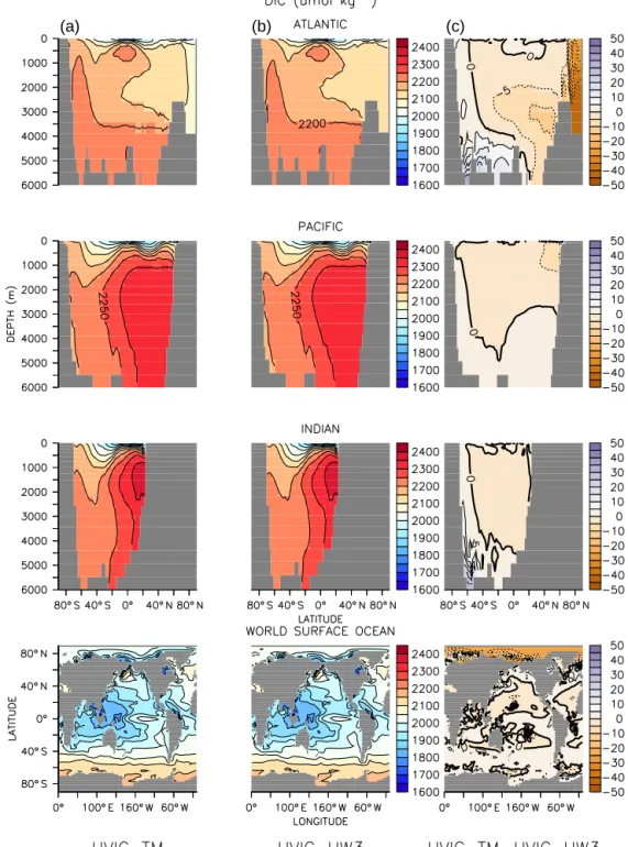
Figure 1.Dissolved inorganic carbon in the offline simulation(a), online simulation(b)and difference between the two(c). Basin profiles are zonal averages.

allel, with details of the parallelism handled by PETSc and

“hidden” from the end user. Additionally, the interface is implemented in a generic fashion, with the potential to “mix- and-match” circulation (transport matrices) and biogeochemical models.

To apply the TMM code to a particular biogeochemical problem essentially requires providing a routine that takes as

input vertical “profiles” of tracer concentrations at a horizontal location at the current time step (along with corresponding variables such as layer thickness, temperature, wind speed, etc., at that location), and returns profiles of the biogeochemical tendency term,q. In practice, coupling an existing biogeochemical model such as the one in UVic ESCM to the TMM framework involves writing a “wrapper” routine that

(5)

(a) (b) (c)

(d) (e) (f)

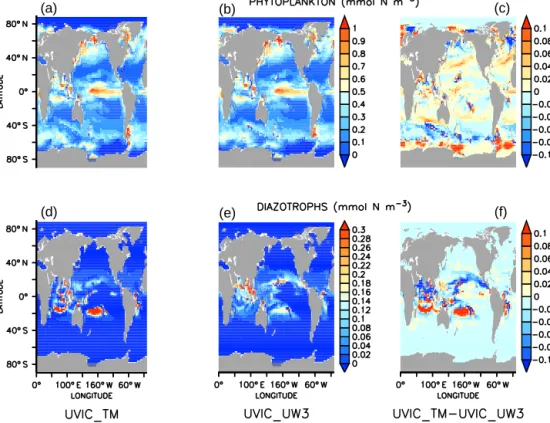
Figure 2.Annually averaged surface phytoplankton (top) and diazotroph (bottom) biomass in mmol N m⁻³. Rightmost plots are differences between offline and online biomass.

serves as an interface between the TMM driver (written in C) and the biogeochemical code (typically written in some dialect of Fortran).

While the specific implementation of the wrapper will de- pend on the details of the biogeochemical model, in general it performs three main tasks. First, it copies required data from TMM arrays (that are passed as input arguments to the wrapper routine) to those of the biogeochemical model. Sec- ond, it calls the actual routine that computes biogeochemical source/sink terms (q). Normally, this routine would be called from the time-stepping loop of the model in which the biogeochemical model is embedded. Third, as these tendency terms are stored in arrays in the biogeochemical model, the wrapper copies them to arrays that are passed back to the TMM driver (as output arguments to the wrapper routine).

To simplify this exchange of data, the horizontal grid, on the biogeochemical model (and ocean model in which it is embedded), is declared to have a size of 1×1. In essence, the biogeochemical model is treated as a 1-D column model. In the case of UVic ESCM, where the code for physical and biogeochemical models are deeply intertwined, a few minor, additional changes to the original code were also necessary.

Most of these changes were required in order to make available the full set of diagnostics accumulated by UVic ESCM.

See code availability at the end of the article for information on where to download the code.

The offline biogeochemical model is forced with the rele- vant physical and biogeochemical fields taken from the equilibrated online model. In the present case, these are monthly mean wind speed, insolation, sea ice concentration, temperature, salinity, freshwater flux (evaporation, precipitation and runoff), and iron concentration. All fields, including the previously extracted transport matrices (also at monthly mean resolution), are linearly interpolated to the current time step before being applied. The offline model was integrated with a time step of 8 h for 5000 years to equilibrium, with monthly averages of various fields from the final year of this run used for comparison with the equilibrated online simulation.

3 Results and discussion

3.1 Comparison of online and offline simulations 3.1.1 Mean state

We first compare the annual-mean state of the online (UVIC_UW3) and offline (UVIC_TM) simulations, taken from the final year of the corresponding spin-up. A fully stable UVic ESCM simulation with annually repeating seasonal forcing has no inter-annual variability. The surface DIC distribution (Fig. 1) typically differs by less than 5 µmol kg⁻³, although isolated grid points in the Arctic are

(6)

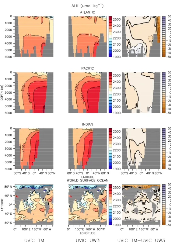
Figure 3.Same as Fig. 1 but for alkalinity.

up to 20 µmol kg⁻³lower in UVIC_TM. In the low latitudes there are grid points with differences of up to 10 µmol kg⁻³ due to minor differences in the phytoplankton distribution between UVIC_TM and UVIC_UW3 (Fig. 2). Diazotroph populations in the Indian and western Pacific oceans are more concentrated in UVIC_TM, with annual average concentrations exceeding 0.3 mmol N m⁻³ at some locations.

Differences in the diazotroph distribution can influence DIC

and alkalinity (Fig. 3) because diazotrophs do not contribute to carbonate export in the model. Diazotrophs are dispro- portionately sensitive to low oxygen levels as oxygen defi- ciency can trigger denitrification, which increases their relative fitness over the general phytoplankton type in our model.

While the global annual average rate of denitrification is higher in the online model (5.63×10⁻¹³mol N m⁻³s⁻¹) than in the offline model (5.55×10⁻¹³mol N m⁻³s⁻¹), the

(7)

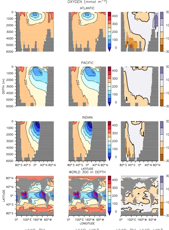
Figure 4.Same as Fig. 1 but for oxygen. Note the maps are plotted at 300 m depth. Suboxic regions (less than 5 mmol m⁻³) are denoted with red boundaries.

offline model has more grid points with very high values (not shown). Small spatial and temporal differences in suboxic conditions in the online and offline models can therefore affect diazotrophs in this region where oxygen levels are already fairly low (Fig. 4). Thus, the distribution of carbon and alkalinity is slightly affected. Note, though, that online–

offline differences in these quantities are restricted to the near-surface and do not extend into the deep ocean.

Similar to DIC, differences in surface alkalinity values rarely exceed 5 µmol kg⁻³ (Fig. 3). Sub-surface alkalinity values in the Arctic are up to 50 µmol kg⁻³ too high in UVIC_TM, likely because of the absence of polar filtering.

(8)

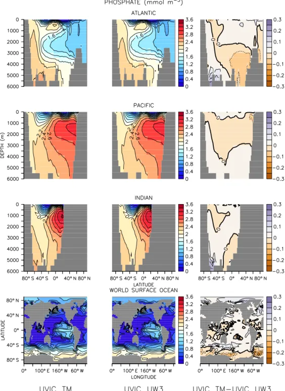
Figure 5.Same as Fig. 1 but for phosphate.

Zonally averaged sections show that alkalinity is otherwise in close agreement between online and offline integrations.

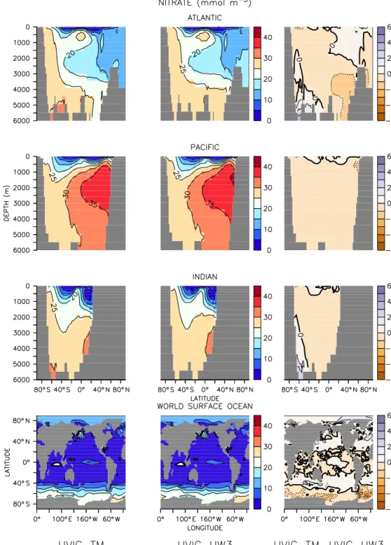
Phosphate and nitrate distributions likewise show negligi- ble differences between models with the exception of polar regions and the water masses closely associated with those regions (Figs. 5 and 6). The UVIC_TM phosphate concentrations are up to 0.2 mmol m⁻³ higher in the deep sub- polar Atlantic and abyssal Southern Ocean, while UVIC_TM

nitrate concentrations are up to 5 mmol m⁻³ higher than UVIC_UW3 in the abyssal Southern Ocean, but up to 5 mmol m⁻³ lower in the deep sub-polar Atlantic. The absence of polar filtering in the offline model is contributing to these differences, as is slightly higher primary production in the offline Southern Ocean, which enhances the biological pump (Fig. 2). This higher primary production may be due to slight differences in the application of external forc-

(9)

Figure 6.Same as Fig. 1 but for nitrate.

ing, which is expected to introduce some bias to regions with strong seasonality. All of the above biases are small relative to discrepancies between the models and observations (see below).

Oxygen distributions in UVIC_TM are up to 50 mmol m⁻³ higher in the deep sub-polar Atlantic and in parts of the surface Arctic compared with UVIC_UW3 (Fig. 4). Aside from

the minor differences at lower latitudes mentioned earlier, these are the only notable mismatches between the offline and online integrations for oxygen.

The above results are summarized in a spatially integrated manner via the Taylor plots and associated tables shown in Fig. 7. Evidently, the root mean square (RMS) difference between the offline and online runs for most variables is quite

(10)

Figure 7. Taylor diagrams for various simulated biogeochemical quantities in the offline model compared with the online one. Different symbols and colors correspond to different ocean basins. For each symbol plotted, the azimuthal angle is the correlation coefficient between the offline and online field, with a correlation coefficient of “1” lying on thexaxis, and the radial distance from the origin is the spatial standard deviation of the field in the offline model. To avoid cluttering the diagram, we plot the standard deviation of the online field as a colored, dashed line so that the online model is the intersection of that line with thexaxis. The distance between that intersection point and any plotted symbol is the centered RMS difference between the offline and online models. The RMS differences are also shown in a table next to each plot along with, for context, the centered RMS difference between the online model and observations (where available).

(11)

(a) (b) (c)

(d) (e) (f)

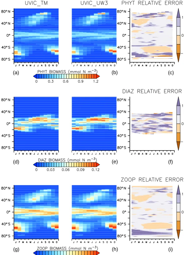
(g) (h) (i)

Figure 8.Zonally averaged surface biomass for phytoplankton (top), diazotrophs (middle), and zooplankton (bottom) as a function of month and latitude in the offline simulation (left column), online simulation (center), and relative difference between the two (right). Relative error is calculated as (UVIC_TM - UVIC_UW3)/UVIC_UW3. Units are mmol N m⁻³.

(12)

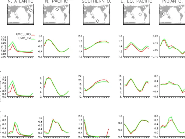
Figure 9.Monthly mean surface phosphate, nitrate, and phytoplankton biomass as a function of calendar month for selected points. The map view indicates the location of the points as diamonds. Models are shown with colors: red is UVIC_UW3, green is UVIC_TM.

small. To put those differences into perspective, also tabulated is the RMS difference between the online simulation and observations, which is seen to be over 10 times larger than the corresponding RMS difference between offline and online runs.

3.1.2 Seasonal cycle

In addition to the time–mean state it is important for any offline approach to capture the seasonal cycle. Figure 8 shows that this is indeed the case for the zonally averaged biomass at the surface. The relative error resulting from small differences in small concentrations can be large, so this comparison is limited to noting that the relative error in biomass generally increases towards the poles, as would be expected based on the discrepancies in annually averaged biogeochemical quantities described earlier.

The timing of seasonal maxima also appear well aligned between offline and online runs when examined at several locations (Fig. 9). The North Pacific, North Atlantic, and Southern Ocean locations in particular display synchronous seasonal timing in nutrients and phytoplankton, although there are small differences in the amplitude at a few locations. This may in part be due to differences in how the bio-

geochemical component of the online and offline models are forced. In the former, instantaneous fields from the ocean and atmosphere are used to drive the biogeochemistry. By con- trast, and similar to other offline schemes, in the TMM time- averaged circulation and forcing fields (insolation, sea ice, wind speed, etc.) are linearly interpolated in time to the current time step before being applied. This averaging, the degree of which (monthly in these experiments) is arbitrary, has the potential to introduce biases, especially in rapidly varying variables such as phytoplankton that are sensitive to non- linearities in the population equations.

3.2 Computational performance of the TMM versus online model

UVic ESCM is a serial code and thus unable to exploit more than one computational core. With the biogeochemical component switched on the model throughput on a typical Linux machine (ours has a 2.6 GHz Sandy Bridge-EP processor) is about∼250 model years per day. (It should be noted that the model was run with the atmospheric energy balance model (EBM) switched on. This adds roughly 20 % to the computational cost of running the model. However, as currently implemented, it is not possible to switch off the EBM in UVic

(13)

ESCM and drive the ocean GCM with prescribed fluxes.) A 5000-year spin-up of the online biogeochemical model thus takes∼3 weeks. On the other hand, the PETSc-based TMM version can run in parallel, even though the underlying biogeochemical code is identical. While we have not carried out a detailed scaling analysis of the TMM version’s performance, a similar 5000-year spin-up can be accomplished in 3.8 h with 256 cores on NCAR’s Yellowstone IBM iDataPlex cluster, and in 5.2 h with 160 cores on GEOMAR/Kiel Uni- versity’s NEC HPC machine.

4 Conclusions

This study investigates the extent to which the transport matrix method, a scheme for offline simulation of ocean biogeochemical tracers, can reproduce the corresponding online model, specifically an NPZD-type biogeochemical model embedded into UVic ESCM. While the focus is on a detailed comparison of the offline run with the online one, we also describe the mechanics of extracting transport matrices from UVic ESCM and coupling its biogeochemical model to the TMM framework. As the steps required for both aspects are quite general, this may be useful for researchers interested in applying the TMM to other ocean and biogeochemical models.

We show that the TMM version captures reasonably well both the time–mean state and seasonal cycle of biogeochemical tracers of the online model. Small discrepancies arise at high latitudes due to the absence of polar filtering in the offline model. Differences also arise from the time averaging (monthly in these experiments) of forcing fields and the circulation embedded in the transport matrices, although the degree of averaging can be varied to suit the situation. Phyto- plankton are especially sensitive to this time averaging, with the impact on most biogeochemical tracers being limited to the surface ocean. These differences are generally much smaller than biases in the models with respect to observations.

While UVic ESCM is a serial model, the TMM version can be run in parallel without any modifications to the underlying code. Simulations performed with the TMM are thus orders of magnitude faster making it possible to routinely perform long spin-ups of UVic ESCM biogeochemistry in a few hours rather than weeks. A recent study (Séférian et al., 2016) highlighting the importance of adequate spin-ups sug- gests that this could be beneficial even for earth system models that are already parallelized, especially with the advent of many-core hardware architectures, such as general purpose graphics processing units (GPGPUs) to which the TMM has been recently ported (Siewertsen et al., 2013). Moreover, the speed-up opens up the possibility of systematically testing different parameterizations in complex, global biogeochemical models, or even optimizing such models against data as has been recently accomplished for a slightly simpler model by Kriest et al. (2017). While the results presented here are for a particular model, they should be broadly applicable to other global models of similar complexity.

Code availability. The specific version of the offline biogeochemical model code, transport matrices and other data used for the simulations described in this paper are available from https://thredds.geomar.de/thredds/catalog/open_access/kvale_

et_al_2017_gmdd/catalog.html or http://kelvin.earth.ox.ac.uk/spk/

Research/TMM/Kvale_etal_2017_GMDD.tar.gz. (The most recent version of the code and transport matrices from various circulation models are distributed from https://github.com/samarkhatiwala/

tmm.) The archive also contains model output and scripts used to create the figures in this manuscript.

(14)

2438 K. F. Kvale et al.: Online–offline comparison Appendix A: Comparison of third-order upwind and

flux-corrected transport online runs

Here we discuss the changes due to switching from UVic ESCM’s default, non-linear flux-corrected transport scheme (UVIC_FCT) to the third-order linear advection scheme (UVIC_UW3). As noted in Sect. 2.1, only the vertical diffusivity was increased when switching to the UW3 scheme to bring the MOC strength back closer to observations; all other parameters were left at values previously tuned to the default FCT scheme.

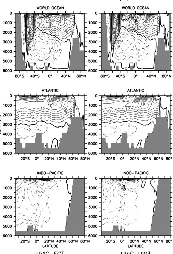
Figure A1 compares the global, Atlantic, and Indo-Pacific meridional overturning circulation of the model for the two schemes. Antarctic Bottom Water (AABW) formation in the Southern Ocean occurs with an counterclockwise stream function of 2 Sv poleward of a Deacon cell reaching 32 Sv near the surface in both cases. AABW extends northward into the Atlantic with an counterclockwise stream function of up to 2 Sv below 3000 m depth, and up to 6 Sv in the deep Indo-Pacific, with only minor differences in isolines between the two schemes. North Atlantic Deep Water (NADW) over- lies AABW and reaches a maximum of 16 Sv around 30^◦N and 1000 m depth. Overturning is slightly stronger in this region in UVIC_UW3 than in UVIC_FCT, with the zone within the 14 Sv isoline extending from about 5 to 40^◦N in the former, as opposed to roughly 20 to 40^◦N in the latter.

This is mirrored by the distribution of natural radiocarbon (Fig. A2), which shows a larger North Atlantic contribution in UVIC_UW3 leading to generally younger deep ocean radiocarbon ages in this configuration relative to UVIC_FCT.

Sea surface temperature and zonally averaged sections of potential temperature in each ocean basin show few differences between UVIC_UW3 and UVIC_FCT (Fig. A3). The most notable one is in the abyssal Atlantic, where the 4^◦C isotherm extends 1000 m deeper and the 0^◦C isotherm extends 20^◦ farther north in UVIC_UW3, consistent with a stronger NADW formation and more energetic AABW in this simulation. Both cases show a 1–2^◦C cold bias in the abyssal Atlantic and Pacific basins, and a warm bias of up to 5^◦C in the tropics, with respect to an observational climatology (World Ocean Atlas; Locarnini et al., 2010). Similarly, salinity differences between the two schemes are most notable in the Atlantic basin (Fig. A4). UVIC_UW3 AABW is 0.5 psu fresher than UVIC_FCT, though the northern North Atlantic salinity is more similar. Surface salinity in both cases is generally too low relative to observations (Antonov et al., 2010), while surface and deep North Atlantic salinity is 0.5–1.0 psu too high.

The Taylor diagrams shown in Fig. A5 highlight the impact of different advection schemes on biogeochemistry. As in the physical model, the biogeochemical model parameters were previously tuned for the FCT advection scheme; no additional tuning was performed for the UW3 scheme. We therefore expect UVIC_FCT to be in closer agreement to observations than UVIC_UW3, although, generally, differences between UVIC_FCT and UVIC_UW3 biogeochemistry are much smaller than their mismatch with observations. The largest differences are in nitrate and alkalinity, both of which are sensitive to small differences in oxygen via biological processes discussed in Sect. 3.1.

(15)

Figure A1.Meridional overturning in flux-corrected transport (UVIC_FCT) and third-order upwind advection (UVIC_UW3) online models.

Positive (negative) values indicate clockwise (counterclockwise) circulation.

(16)

Figure A2.Background radiocarbon in online models UVIC_FCT and UVIC_UW3 compared with gridded observations from the GLODAP dataset (Key et al., 2004). Basin profiles are zonal averages.

(17)

Figure A3.Potential temperature in online models UVIC_FCT and UVIC_UW3 compared with the World Ocean Atlas climatology (Lo- carnini et al., 2010). Basin profiles are zonal averages.

(18)

Figure A4. Salinity in online models UVIC_FCT and UVIC_UW3 compared with the World Ocean Atlas climatology (Antonov et al., 2010). Basin profiles are zonal averages.

(19)

Figure A5.Taylor diagrams for various simulated biogeochemical quantities in comparison to observations (World Ocean Atlas climatology Garcia et al., 2010a, b) showing the impact of advection scheme. Different symbols and colors correspond to different ocean basins, with light shaded symbols representing UVIC_UW3 and dark shaded ones UVIC_FCT. For each symbol plotted, the azimuthal angle is the correlation coefficient between the simulated and observed field, with a correlation coefficient of “1” lying on thexaxis, and the radial distance from the origin is the spatial standard deviation of that field. To avoid cluttering the diagram, we plot the standard deviation of the corresponding observation as a colored, dashed line so that the observation lies on the intersection of that line with thexaxis. The distance between that intersection point and any plotted symbol is the centered RMS difference between the model and data. For clarity these RMS values are also tabulated in the figure.

(20)

2444 K. F. Kvale et al.: Online–offline comparison Author contributions. SK and KK wrote the paper (with comments

by HD, IK, and AO), implemented the matrix interface and extraction, and performed the simulations. HD re-tuned the online model to use a linear advection scheme and assisted with interpretation.

AO, IK and SK conceived the project.

Competing interests. The authors declare that they have no conflict of interest.

Acknowledgements. This work is a contribution to DFG-supported project SFB754 and to the research platforms of DFG cluster of excellence The Future Ocean. Khatiwala was supported in part by US NSF grant OCE 12-34971 and UK NERC grant NE/K015613/1. Computing resources (ark:/85065/d7wd3xhc) were provided by the Climate Simulation Laboratory at NCAR’s Computational and Information Systems Laboratory, sponsored by the National Science Foundation and other agencies. We also gratefully acknowledge computer resources made available at Kiel University, technical consultation with Michael Eby and figure scripts by Andreas Schmittner.

Edited by: Paul Halloran

Reviewed by: three anonymous referees

References

Antonov, J., Seidov, D., Boyer, T. P., Locarnini, R. A., Mishonov, A., Garcia, H., Baranova, O., Zweng, M. M., and Johnson, D.:

World Ocean Atlas 2009, Volume 2: Salinity, Tech. rep., NOAA Atlas NESDIS 69, U.S. Government Printing Office, Washing- ton, DC, 2010.

Balay, S., Gropp, W. D., McInnes, L. C., and Smith, B. F.: PETSc Users Manual, Tech. Rep. ANL-95/11 – Revision 2.1.5, Argonne National Laboratory, 2003.

Coleman, T. F. and Moré, J. J.: Estimation of sparse Jacobian matrices and graph coloring problems, SIAM J. Numer. Anal., 20, 187–209, 1983.

Curtis, A. R., Powell, M. J. D., and Reid, J. K.: On the estimation of sparse Jacobian matrices, J. Inst. Math. Appl., 13, 117–119, 1974.

Duteil, O., Koeve, W., Oschlies, A., Bianchi, D., Galbraith, E., Kri- est, I., and Matear, R.: A novel estimate of ocean oxygen utilisa- tion points to a reduced rate of respiration in the ocean interior, Biogeosciences, 10, 7723–7738, https://doi.org/10.5194/bg-10- 7723-2013, 2013.

Eby, M., Zickfeld, K., Montenegro, A., Archer, D., Meissner, K. J., and Weaver, A. J.: Lifetime of Anthropogenic Climate Change: Millennial Time Scales of Potential CO₂ and Sur- face Temperature Perturbations, J. Climate, 22, 2501–2511, https://doi.org/10.1175/2008JCLI2554.1, 2009.

Garcia, H., Locarnini, R. A., Boyer, T. P., Antonov, J., Baranova, O., Zweng, M. M., and Johnson, D.: World Ocean Atlas 2009, Volume 3: Dissolved Oxygen, Apparent Oxygen Utilization, and Oxygen Saturation, Tech. rep., NOAA Atlas NESDIS 70, U.S.

Government Printing Office, Washington, D.C., 2010a.

Garcia, H., Locarnini, R. A., Boyer, T. P., Antonov, J., Zweng, M. M., Baranova, O., and Johnson, D.: World Ocean Atlas 2009, Volume 4: Nutrients (phosphate, nitrate, silicate), Tech. rep., NOAA Atlas NESDIS 71, U.S. Government Printing Office, Washington, D.C., 2010b.

Graven, H. D., Gruber, N., Key, R., Khatiwala, S., and Gi- raud, X.: Changing controls on oceanic radiocarbon: New insights on shallow-to-deep ocean exchange and anthropogenic CO₂ uptake, J. Geophys. Res., 117, C10005, https://doi.org/10.1029/2012JC008074, 2012.

Griffies, S., Harrison, M., Pacanowski, R., and Rosati, A.: A Tech- nical Guide to MOM4, GFDL ocean group technical report No.

5, NOAA/Geophysical Fluid Dynamics Laboratory, 2008.

Gropp, W. D., Kaushik, D. K., Keyes, D. E., and Smith, B. F.: Towards Realistic Performance Bounds for Implicit CFD Codes, in: Parallel Computational Fluid Dynamics, Proceedings of the Parallel CFD’99 Conference, Elsevier, https://doi.org/10.1016/B978-044482851-4.50030-X, 2000.

Holland, W., Chow, J., and Bryan, F.: Application of a third-order upwind scheme in the NCAR Ocean Model, J. Climate, 11, 1487–1493, https://doi.org/10.1175/1520- 0442(1998)011<1487:AOATOU>2.0.CO;2, 1998.

Jones, K., Khatiwala, S., van de Flierdt, T., Hemming, S., and Gold- stein, S.: Modeling the distribution of Nd isotopes in the oceans using an ocean general circulation model, Earth Planet. Sci. Lett., 272, 610–619, 2008.

Keller, D. P., Oschlies, A., and Eby, M.: A new marine ecosystem model for the University of Victoria Earth Sys- tem Climate Model, Geosci. Model Dev., 5, 1195–1220, https://doi.org/10.5194/gmd-5-1195-2012, 2012.

Keller, D. P., Kriest, I., Koeve, W., and Oschlies, A.: Southern Ocean biological impacts on global ocean oxygen, Geophys. Res.

Lett., 43, 6469–6477, https://doi.org/10.1002/2016GL069630, 2016.

Key, R., Kozyr, A., Sabine, C., Lee, K., Wanninkhof, R., Bullister, J., Feely, R., Millero, F., and Mordy, C.: A global ocean carbon climatology: Results from GLODAP, Global Biogeochem. Cy., 18, GB4031, https://doi.org/10.1029/2004GB002247, 2004.

Khatiwala, S.: A computational framework for simulation of biogeochemical tracers in the ocean, Global Biogeochem. Cy., 21, GB3001, https://doi.org/10.1029/2007GB002923, 2007.

Khatiwala, S.: Fast spin up of Ocean biogeochemical models using matrix-free Newton-Krylov, Ocean Model., 23, 121–129, https://doi.org/10.1016/j.ocemod.2008.05.002, 2008.

Khatiwala, S., Visbeck, M., and Cane, M.: Accelerated simulation of passive tracers in ocean circulation models, Ocean Modell., 9, 51–69, 2005.

Koeve, W. and Kähler, P.: Oxygen utilization rate (OUR) underes- timates ocean respiration: A model study, Global Biogeochem.

Cy., 30, 1166–1182, https://doi.org/10.1002/2015GB005354, 2016.

Koeve, W., Duteil, O., Oschlies, A., Kähler, P., and Segschneider, J.: Methods to evaluate CaCO₃cycle modules in coupled global biogeochemical ocean models, Geosci. Model Dev., 7, 2393–

2408, https://doi.org/10.5194/gmd-7-2393-2014, 2014.

Koeve, W., Wagner, H., Kähler, P., and Oschlies, A.:¹⁴C-age tracers in global ocean circulation models, Geosci. Model Dev., 8, 2079–

2094, https://doi.org/10.5194/gmd-8-2079-2015, 2015.

(21)

Kriest, I. and Oschlies, A.: MOPS-1.0: towards a model for the regulation of the global oceanic nitrogen budget by marine biogeochemical processes, Geosci. Model Dev., 8, 2929–2957, https://doi.org/10.5194/gmd-8-2929-2015, 2015.

Kriest, I., Khatiwala, S., and Oschlies, A.: Towards an assessment of simple global marine biogeochemical models of different complexity, Prog. Oceanogr., 86, 337–360, https://doi.org/10.1016/j.pocean.2010.05.002, 2010.

Kriest, I., Oschlies, A., and Khatiwala, S.: Sensitiv- ity analysis of simple global marine biogeochemical models, Global Biogeochem. Cy., 26, GB2029, https://doi.org/10.1029/2011GB004072, 2012.

Kriest, I., Sauerland, V., Khatiwala, S., Srivastav, A., and Os- chlies, A.: Calibrating a global three-dimensional biogeochemical ocean model (MOPS-1.0), Geosci. Model Dev., 10, 127–154, https://doi.org/10.5194/gmd-10-127-2017, 2017.

Liang, J., Deutsch, C., McWilliams, J. C., Baschek, B., Sullivan, P. P., and Chiba, D.: Parameterizing bubble-mediated air-sea gas exchange and its effect on ocean ventilation, Global Bio- geochem. Cy., 27, 894–905, https://doi.org/10.1002/gbc.20080, 2013.

Locarnini, R. A., Mishonov, A., Antonov, J., Boyer, T. P., Gar- cia, H., Baranova, O., Zweng, M. M., and Johnson, D.: World Ocean Atlas 2009, Volume 1: Temperature, Tech. rep., NOAA Atlas NESDIS 68, U.S. Government Printing Office, Washing- ton, D.C., 2010.

Marshall, J., Adcroft, A., Hill, C., Perelman, L., and Heisey, C.: A finite-volume, incompressible Navier-Stokes model for studies of the ocean on parallel computers, J. Geophys. Res., 102, 5733–

5752, 1997.

Nicholson, D. P., Emerson, S. R., Khatiwala, S., and Hamme, R. C.:

An inverse approach to estimate bubble-mediated air-sea gas flux from inert gas measurements, in: The 6th International Sympo- sium on Gas Transfer at Water Surfaces, edited by: Komori, S., McGillis, W., and Kurose, R., Kyoto University Press, 223–237, 2011.

Nicholson, D. P., Khatiwala, S., and Heimbach, P.: Noble gas tracers of ventilation during deep water formation in the Weddell Sea, in:

The 7th International Symposium on Gas Transfer at Water Sur- faces, IOP Conference Series: Earth and Environmental Science, https://doi.org/10.1088/1755-1315/35/1/012019, 2016.

Priess, M., Koziel, S., and Slawig, T.: Marine ecosystem model calibration with real data using enhanced surrogate-based optimization, J. Comput. Sci., 4, 423–437, https://doi.org/10.1016/j.jocs.2013.04.001, 2013a.

Priess, M., Piwonski, J., Koziel, S., Oschlies, A., and Slawig, T.: Ac- celerated parameter identification in a 3D marine biogeochemical model using surrogate-based optimization, Ocean Mod- ell., 68, 22–36, https://doi.org/10.1016/j.ocemod.2013.04.003, 2013b.

Resplandy, L., Keeling, R. F., Stephens, B. B., Bent, J. D., Ja- cobson, A., Rodenbeck, C., and Khatiwala, S.: Constraints on oceanic meridional heat transport from combined measurements of oxygen and carbon, Clim. Dynam., 47, 3335–3357, https://doi.org/10.1007/s00382-016-3029-3, 2016.

Séférian, R., Gehlen, M., Bopp, L., Resplandy, L., Orr, J. C., Marti, O., Dunne, J. P., Christian, J. R., Doney, S. C., Ilyina, T., Lind- say, K., Halloran, P. R., Heinze, C., Segschneider, J., Tjiputra, J., Aumont, O., and Romanou, A.: Inconsistent strategies to spin up models in CMIP5: implications for ocean biogeochemical model performance assessment, Geosci. Model Dev., 9, 1827–

1851, https://doi.org/10.5194/gmd-9-1827-2016, 2016.

Siberlin, C. and Wunsch, C.: Oceanic tracer and proxy time scales revisited, Clim. Past, 7, 27–39, https://doi.org/10.5194/cp-7-27- 2011, 2011.

Siddall, M., Khatiwala, S., van de Flierdt, T., Jones, K., Goldstein, S., Hemming, S., and Anderson, R. F.: Towards explaining the Nd paradox using reversible scavenging in an ocean general circulation model, Earth Planet. Sci. Lett., 274, 448–461, 2008.

Siewertsen, E., Piwonski, J., and Slawig, T.: Porting marine ecosystem model spin-up using transport matrices to GPUs, Geosci.

Model Dev., 6, 17–28, https://doi.org/10.5194/gmd-6-17-2013, 2013.

Vance, D., Little, S. H., de Souza, G. F., Khatiwala, S., Lohan, M. C., and Middag, R.: Silicon and zinc biogeochemical cycles coupled through the Southern Ocean, Nat. Geosci., 10, 202–206, https://doi.org/10.1038/ngeo2890, 2017.

Weaver, A. and Eby, M.: On the numerical implementation of advection schemes for use in conjunction with various mixing parameterizations in the GFDL ocean model, J.

Phys. Oceanogr., 27, 369–377, https://doi.org/10.1175/1520- 0485(1997)027<0369:OTNIOA>2.0.CO;2, 1997.

Weaver, A., Eby, M., Wiebe, E., Bitz, C., Duffy, P., Ewen, T., Fan- ning, A., Holland, M., MacFadyen, A., Matthews, H., Meissner, K., Saenko, O., Schmittner, A., Wang, H., and Yoshimori, M.:

The UVic Earth System Climate Model: Model description, climatology, and applications to past, present and future climates, Atmos.-Ocean, 39, 361–428, 2001.

Weber, T. S. and Deutsch, C.: Ocean nutrient ratios governed by plankton biogeography, Nature, 467, 550–554, 2010.

Wilson, J. D., Ridgwell, A., and Barker, S.: Can organic matter flux profiles be diagnosed using remineralisation rates de- rived from observed tracers and modelled ocean transport rates?, Biogeosciences, 12, 5547–5562, https://doi.org/10.5194/bg-12- 5547-2015, 2015.