IOCCG Ocean Optics and Biogeochemistry Protocols for Satellite Ocean Colour Sensor Validation

(1)

(2)

IOCCG Ocean Optics and Biogeochemistry Protocols for Satellite Ocean Colour Sensor Validation

IOCCG Protocol Series Volume 4.0, 2019

Inherent Optical Property Measurements and Protocols:

Best Practices for the Collection and Processing of Ship- Based Underway Flow-Through Optical Data (v4.0)

Report of a NASA-sponsored workshop with contributions from:

Emmanuel Boss University of Maine, School of Marine Sciences, ME, USA Nils Haëntjens University of Maine, School of Marine Sciences, ME, USA Steven G. Ackleson Naval Research Laboratory, Washington, DC, USA Barney Balch Bigelow Laboratory for Ocean Sciences, ME , USA

Alison Chase University of Maine, School of Marine Sciences, ME, USA Giorgio Dall’Olmo Plymouth Marine Laboratory, The Hoe, Plymouth, UK Scott Freeman NASA Goddard Space Flight Center, Greenbelt, MD, USA Yangyang Liu Alfred Wegener Institute, Bremerhaven, Germany

James Loftin University of Maine, School of Marine Sciences, ME, USA Wendy Neary University of Maine, School of Marine Sciences, ME, USA Norman Nelson University of California, Santa Barbara, CA, USA

Mike Novak NASA Goddard Space Flight Center, Greenbelt, MD, USA Wayne H. Slade Sequoia Scientific, Inc., Bellevue, WA, USA

Christopher Proctor NASA Goddard Space Flight Center, Greenbelt, MD, USA Philippe Tortell University of British Columbia, Vancouver, Canada Toby K. Westberry Oregon State University, Corvallis, OR, USA

Edited by:

Aimee R. Neeley and Antonio Mannino

(3)

Correct citation for this volume:

IOCCG Protocol Series (2019). Inherent Optical Property Measurements and Protocols:

Best Practices for the Collection and Processing of Ship-Based Underway Flow-Through Optical Data. Boss, E., Haëntjens, N., Ackleson, S.G., Balch, B., Chase, A., Dall’Olmo, G., Freeman, S., Liu, Y., Loftin, J., Neary, W., Nelson, N., Novak, M., Slade, W., Proctor, C., Tortell, P., and Westberry. T. IOCCG Ocean Optics and Biogeochemistry Protocols for Satellite Ocean Colour Sensor Validation, Volume 4.0, edited by A. R. Neeley and A.

Mannino, IOCCG, Dartmouth, NS, Canada. http://dx.doi.org/10.25607/OBP-664

Acknowledgements:

Support for this work and the workshop that initiated this report was provided by NASA OBB grant number NNX15AC08G to E. Boss. The authors acknowledge the assistance of Collin Roesler, Gianluca Volpe, Aimee Neeley, Antonio Mannino, and Venetia Stuart for their careful review of this report, which resulted in substantial improvements. The authors also thank the Associate Editorial Peer-Reviewers for their constructive comments on this document

Gianluca Volpe National Research Council (CNR), Italy

Collin Roesler Bowdoin College, Dept. Earth & Oceanographic Science, ME, USA

http://www.ioccg.org

Published by the International Ocean Colour Coordinating Group (IOCCG), Dartmouth, NS, Canada, in conjunction with the National Aeronautics and Space Administration (NASA).

Doi: http://dx.doi.org/10.25607/OBP-664

©IOCCG 2019

(4)

Inherent Optical Property Measurements and Protocols:

Best practices for the collection and processing of ship-based underway flow-through optical data

E. Boss,¹ N. Haëntjens,¹ S.G. Ackleson,² B. Balch,³ A. Chase,¹ G. Dall’Olmo,⁴ S.

Freeman,^5,6 Y. Liu,⁷ J. Loftin,¹ W. Neary,¹ N. Nelson,⁸ M. Novak,^5,6 W. Slade,⁹ C.

Proctor,^5,6 P. Tortell,¹⁰ and T. Westberry¹¹

1University of Maine, Orono, ME, 04469, USA

2Naval Research Laboratory, Washington, DC 20032, USA

3Bigelow Laboratory for Ocean Sciences, East Boothbay, ME 04544, USA

4Plymouth Marine Laboratory, Plymouth, UK

5NASA Goddard Space Flight Center, Code 616, Greenbelt, MD 20771, USA

6Science Systems and Applications, Inc. Lanham, MD 20706, USA

7Alfred Wegener Institute Helmholtz Center for Polar and Marine Research, 27570 Bremerhaven, Germany

8University of California Santa Barbara, Santa Barbara, CA 93106, USA

9Sequoia Scientific, Inc., 2700 Richards Road, Suite 107, Bellevue, WA, 98005, USA

10University of British Columbia, Vancouver, BC, Canada

11Oregon State University, Corvallis, OR 97331, USA

1. Introduction

Thermosalinographs have collected continuous flow-through measurements of temperature and salinity for decades (e.g., Henin and Grelet 1996), leading to well-established protocols for quality control, archiving, and distribution of such underway data.¹ Chlorophyll fluorescence has also been integrated into such systems, with the first underway flow-through fluorometry dating back to the late 1960s (Lorenzen 1966).

More recently, several research groups have begun collecting additional optical data (beyond fluorescence) using the flow-through systems installed on research vessels and ships of opportunity to take advantage of the availability of sea water pumped into the vessel (we do not discuss tethered systems here). These “in-line” or “underway” systems provide data at spatial resolutions on the order of 10–100 m, measurement scales that are not accessible with standard hydrographic surveys and enable characterization of sub-pixel variability in satellite ocean color (OC) data. Thus, data collected using this approach are useful for targeted science questions, but also for large-scale calibration/validation of satellite OC products (Werdell et al. 2013).

Optical data are useful for the derivation of biogeochemical quantities through proxy relationships. These have been derived through relationships between particulate absorption spectra and pigments (e.g., Chase et al. 2013, Brewin et al. 2016, Liu et al. 2019), particulate attenuation spectra and a particle size proxy (Boss et al. 2018), particulate attenuation and backscattering at a red wavelength (e.g., 650 nm), and particulate organic carbon (Cetinic et al.

2012 and ref. therein) as well as phytoplankton carbon (Graff et al. 2015). One should always verify that proxy relationships are appropriate for the region in which they are applied.

The growing number of research groups making these measurements demonstrates a need to provide coordinated data collection and processing protocols to standardize methodology and data quality. To share such knowledge, a workshop was organized in 2015 as part of a funded NASA Plankton, Aerosol, Cloud, ocean Ecosystem (PACE) science team proposal where many

1 http://www.gosud.org/, http://ocean.ices.dk/data/underway/underway.htm

(6)

of the co-authors discussed the systems they use. Here we present the essential issues associated with in-line data collection, provide recommendations on best practices for collection and processing, and report on available hardware and processing software.

This report is organized as follows: First, we discuss the instruments and hardware associated with deploying an in-line system and a number of considerations that can affect data quality assurance and quality control (QA/QC). Second, we describe the issues associated with processing of data from specific optical sensors that have been deployed in-line and the software available for data processing.

2. Optical Sensors Used in In-Line Systems

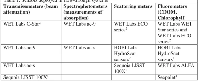
The easiest optical sensors to integrate into underway systems are those designed for flowing or pumped samples, such as flow-through fluorometers and transmissometers. Other optical sensors can be integrated into underway systems using flow cells available as options from manufacturers, or they can be custom-built. Sensors included in underway systems range from transmissometers and spectrophotometers to scattering meters and fluorometers (Table 1).

Table 1: Sensors deployed in flow-through systems Transmissometers (beam

attenuation)

Spectrophotometers (measurements of absorption)

Scattering meters Fluorometers (CDOM, Chlorophyll) WET Labs C-Star¹ WET Labs ac-9 WET Labs ECO

series²

WET Labs WET Star series and WET Labs ECO series²

WET Labs ac-9 WET Labs ac-s HOBI Labs

HydroScat sensors²

HOBI Labs HydroScat sensors²

WET Labs ac-s Sequoia LISST

100X¹

WET Labs ALFA

Sequoia LISST 100X¹ Seapoint¹

Notes:

WET Labs has been acquired by Sea-Bird Scientific

1Requires manufacturer-supplied flow cell or chamber

2Requires custom-built chamber or tank to contain instrument sample volume

3. Ancillary Measurements for In-Line Systems

A GPS must be logged simultaneously with the measurements so that the location and time of each measurement is recorded. A GPS antenna that connects to a USB port can be

purchased for ~$20 USD and used to automatically synchronize the logging computer time. Daily synchronization of all logging devices is necessary to ensure instrument data is merged

appropriately during post-processing.

Since some optical measurements (absorption and attenuation, especially in the red and NIR) require temperature and salinity corrections, a thermosalinograph (typically a Sea-Bird SBE 45 or SBE 21) or equivalent should be part of the in-line system. A temperature sensor is

typically installed near the intake to get the actual in situ temperature.

(7)

A flow meter that records real-time flow information is another critical component of an in-line system. It provides the means to compute the system residence time as well as critical information to evaluate when to replace filters and help with assigning time lags between

instruments deployed in series prior to merging their data. Flow meters can be built with low cost components² or ordered from sensor manufacturers (e.g., FlowControl-Lab, Sequoia Scientific, Inc.).

4. Water System Considerations

4.1 Water source

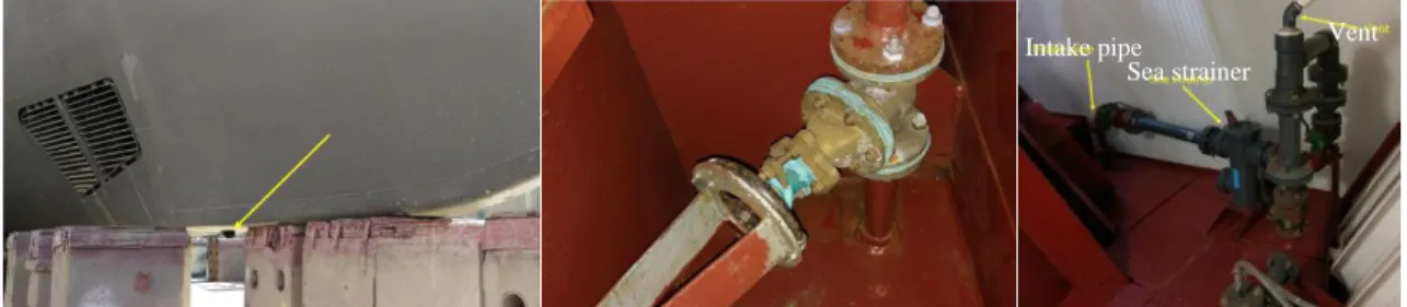
Sample seawater typically enters a vessel from a “sea chest,” a rectangular or cylindrical recess in the hull of the vessel that provides an intake reservoir from which seawater is drawn, or directly via a thru-hull fitting (Figs. 1–3). A location at the ship’s bow or keel is preferred to reduce the amount of contact between the seawater and the vessel. In the case of a sea chest, a metal grating separates the open ocean from the sea chest, dampening the exchange of water and excluding large debris (centimeters in size) that might clog any downstream pump or plumbing.

To measure properties with the in-line system that are as close as possible to those in the water around the ship, it is critical to keep the sea chest clean and not let it become fouled by filter- feeding organisms, rust, or other contaminants. This can be difficult to assess without inspection by a diver. Vessels with thru-hull intakes (e.g., schooner Tara and R/V Atlantis, Figs. 2–3) typically pump the seawater through a strainer basket (mesh size ~ 3–4 mm) and a vent loop is installed to release accumulated air. From pure dilution considerations, a higher flow rate of the water prior to the flow-through optics and positioning the optical system close to the intake will reduce the effect of contamination in the signal.

Figure 1. Moon pool aka Straza Tower (center and left), custom intake (center), and the compressed air driven diaphragm pump and hose installed for the flow-through system on the Atlantic Explorer by Norm Nelson.

Figure 2. Intake scoop on the bottom of the vessel (left), intake pipe (center), and sea strainer debubbling and venting loop (right) of the R/V Atlantis.

2 e.g., https://www.bc-robotics.com/shop/liquid-flow-meter/

Intake pipe Sea strainer pipe

Vent

(8)

4.2 Feeding pump

Impeller pumps are the most common pumps used on research vessels (and UNOLS vessels in particular in the U.S.) and can adversely affect particle assemblages, with observed changes in concentration, composition, and particle size (Cetinic et al. 2016). Diaphragm and peristaltic pumps are recommended to minimize artifacts introduced by the pump; screw pumps may also be good, but currently there is no information regarding the application of such pumps.

Both past (Fig. 3b–c in Westberry et al. 2010) and recent comparisons of particle images

collected from underway systems and Niskin bottles found very good agreement between the two water sources when using diaphragm pumps (comparable optical properties and size distributions of particles analyzed from water collected by rosette and from the in-line system).

Figure 3. Underway instrument loop and pump on the R/V Atlantis during NAAMES 03.

We have experience with the following pumps; the field campaign or R/V is in parentheses for reference:

1. ARO air-operated diaphragm pumps (SABOR, NAAMES, Fig. 3)³ 2. Shurflo electric pump (Tara)⁴

3. Graco Husky 1050E pump (NAAMES)⁵

4. Tapflo air-operated pump (KORUS-OC, Sea2Space)⁶

Note that new or modified feeding pumps and downstream scientific instrument installations often have initial problems with bubbles in the sample flow, a condition that negatively affects the measurements of particulate optical properties. Adjusting the flow by increasing flow rates through instruments, including a debubbler (see Section 5.2), and adding slight backpressure downstream of the instruments often solves the bubble problem (although in some sea states it will not). Moreover, avoiding right-angle turns in pipes and tubing, and

ensuring sealed connections, as well as free flow of the outlet, are essential to preventing bubbles.

3 http://www.arozone.com/en/products/diaphragm-pumps.html

4 https://www.svb24.com/en/shurflo-pressurized-water-pump-aqua-king-ii-standard-3-0.html

5 http://www.graco.com/content/dam/graco/ipd/literature/flyers/345088/345088ENEU-A.pdf

6 http://www.tapflo.com/en/diaphragm-pumps/pe-ptfe-pumps/t100

(9)

Vigilance is required as ship operations (e.g., maintaining station, bow thrusters) or an increase in sea state while underway may also introduce bubbles in the flowing seawater. Note that the flow from peristaltic, and especially diaphragm pumps, may be pulsed. Semi-rigid and softer tubing tends to dampen this pulsation; the bubble prevention methods described here do not appear to adversely affect optical measurements, such as fluctuations in raw measurements at the pulsation frequency or significant particle breakage.

4.3 Plumbing

Plumbing should be cleaned prior to leaving the dock, typically by flushing the plumbing system with bleach followed by rinsing it with fresh water or, if possible, by replacing the tubing within the system. Plumbing that is not bleached and thoroughly flushed has been found to bias O2 and pCO2 and is likely to also bias optical measurements (Juranek et al. 2010).

Reducing the amount of contact between the input seawater and plumbing (including sea chest, pump, and plumbing to labs) leads to fewer opportunities to affect the optical properties of measured particles or introduce dissolved substances to the stream. Larger diameter pipes and avoiding sharp angles in the system can reduce shear and particle breakage. Thus, we anticipate better agreement between underway and in situ samples for short and wide pipes compared to long and narrow. While the ship’s plumbing must be cleaned and cannot be changed in most cases, the end connection to the instrument is installed by the operator. Material of fittings such as valves and bulkheads should be approached with caution (i.e., could be metals or plastic, but check for degradation).

The tubing listed below is recommended for ease of installation and to reduce bio- accumulation from occurring in it during a typical five-week expedition:

 Excelon laboratory tubing from US Plastics o Model number 59062⁷

 Tygon R-3603

o Do not use E-3603 as some plasticizers have been removed resulting in rapid fouling

 EJ Beverage Ultra Barrier Silver Bexag 4-6

o More difficult to bend and cut than the tubing mentioned above

Attention must be paid to biofouling in the line as it can affect the quality of the measurements. Lines, adapters, debubblers, and the filter holder can be cleaned with bleach or RBS™ 35 (a laboratory cleaning agent e.g., Thermo-Fisher 27950) and letting them soak in a cleaning solution for a few hours (some users have found RBS to be more effective at removing films). Strategies to assess biofouling while underway are critical, as is a plan for cleaning during deployment. An easy water diversion strategy is recommended to protect instrumentation from bleaching lines.

5. General Considerations

This document includes the University of Maine laboratory checklists for what to do prior to leaving dock (Appendix I) and while at sea (Appendix II). Using these will help address the issues detailed in this report in a timely way to ensure the quality of data collected.

7 www.usplastics.com

(10)

5.1 Flow rate

A flow rate between 2–10 L/min has been found to work well, depending on the instruments being deployed in the underway system and how much water is vented in

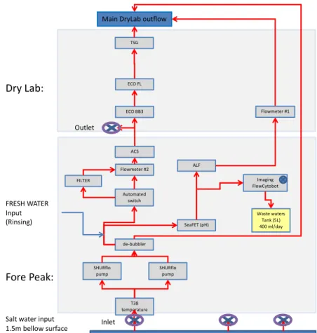
debubbler(s) upstream of the instruments (see below). Flow rate considerations are crucial for assessing delays between different instruments installed in series along the water path. It is important to monitor the flow rate, as well as the pressure within the system, as it provides a diagnostic to check (especially when examining data post-deployment) when measurements change for no apparent reason. An example of a schematic of the in-line system installed on the Tara Polar Circle expedition is shown in Fig. 4.

Figure 4. Schematic of the in-line system installed on the Tara during the Tara Polar Circle expedition.

Figure provided by Marc Picheral.

5.2 Bubbles and debubbling

Warming of the water or cavitation through the path (a sudden reduction of pressure within the water)—in addition to bubbles introduced by turbulence in the plumbing system, bubble entrainment at the ocean surface, and at the intake emerging from the water—can cause bubble formation. During rough seas, significantly more bubbles occur in the system, likely due to exposure of the sea chest to hull turbulence.

In addition to the solutions for bubbles described in the pump section, installing a vortex debubbler (Ocean Instrument Laboratory, Stony Brook University, MSRC Vortex Debubbler,

ALF

Imaging FlowCytobot

SHURflo pump

Automated switch Flowmeter #2

ECO BB3 ECO FL

T38 temperature

TSG

Salt water input 1.5m bellow surface

Main DryLab outflow

Fore Peak:

Dry Lab:

Inlet Outlet

Waste waters Tank (5L) 400 ml/day FILTER

de-bubbler

FRESH WATER Input

(Rinsing) SeaFET (pH)

SHURflo pump ACS

Flowmeter #1

(11)

Model VDB-1⁸) upstream of the instruments to remove bubbles is recommended. The debubblers are manufactured in two sizes: 2- and 3-inch diameter models designed for flow rates of up to 10 or 20 liters per minute, respectively. Customized debubblers are also possible (e.g., -4H-Jena- Engineering GmbH, Germany⁹). Using multiple debubblers in a series reduces the bubble impact in rough seas; however, it increases residence time in the plumbing system and increases the exposure of particles to shear, possibly leading to particle breakage.

Adding a constriction (i.e., valve or section of smaller diameter tubing) at the outlet of the system to create a slight backpressure has been found to help alleviate bubble issues. The

backpressure may expose water leaks elsewhere in the system. Such leaks are important to identify as they are likely points at which air could leak into the system. The installation of a ‘Y’

or tee fitting placed at a high point in the system with a valve is useful to release trapped air (a

“degassing Y”) introduced into the system when changing the filter, especially if positioned between the particle filter and instruments to bleed air. Leaks in ac-meters may be caused by faulty O-rings, which should be inspected, very lightly greased, and replaced as necessary. O- rings should be in every spare kit; note that O-rings are different for the a-detector side compared to all other mating fitting with flow cells and between flow cell and flow sleeve.

5.3 In-line

filters

5.3.1 Particle size fractionation

Filters are used to measure the properties of specific particle size ranges or to use measurements performed with a specific filtered fraction as the blank for larger particles (see Section 5.8). Industrial filters—similar to ones used for drinking water, but typically with tighter specifications, i.e., “absolute-rated”—work well, providing a large filter surface area which does not excessively constrict the flow (e.g., flow could drop by about 40% between total and filtered).

Alternatively, an industrial filter may be used as a pre-filter, then the seawater is passed through a 0.2-m capsule filter. In turbid waters, an additional pre-filter with a wider pore size (e.g., 5-m) can help prevent rapid filter clogging.

5.3.2 Measuring the absorption and attenuation of dissolved matter

The addition of a valve (i.e., either manual or automated) to periodically divert the sample seawater through a particle filter (typically 0.2-m pore size) is recommend to measure the absorption and attenuation of filtered seawater (Fig. 4), and, by difference, obtain “calibration independent” particulate optical properties (Slade et al. 2010). This process assumes that the interpolation between dissolved measurements provides a good estimate of the properties of the dissolved fraction when measurements of unfiltered seawater are made, which could be assessed using a CDOM fluorometer. Such a fluorometer could be used to diagnose fronts and help design a non-linear interpolation. This method of particulate measurements can provide highly sensitive and high-quality measurements of particulate optical properties (Balch et al. 2004; Slade et al.

2010; Werdell et al. 2013; Liu et al. 2018).

Commercial systems for automating filtered seawater measurements are available (e.g., FlowControl-Lab, Sequoia Scientific, Inc.) which also integrate flow rate measurements. If the backscattering sensor is placed after the valve or filter, measurements of the backscattering by the

8 https://www.somas.stonybrook.edu/about/facilities/instrument-laboratory-eshop/msrc-vdb-1-vortex- debubbler/

9 http://www.4h-jena.de/wp-content/uploads/2017/01/4H-Debubbler.pdf

(12)

<0.2-m fraction are obtained in conjunction with that of the water. A fluorometer in-line after the switch is also able to assess the contribution of CDOM to the measured chlorophyll

fluorescence (see Section 7.2). It is also beneficial to increase the frequency of filtered

measurements if working in regions where dissolved optical properties are expected to be more variable, such as in shelf waters or along frontal boundaries. Typically, 12–24 filtered

measurement intervals per day (10–15 minutes per measurement) are more than sufficient in open waters.

5.3.3 Practical advice on filters

Frequently switching between filtered and non-filtered operation following a filter change helps reduce bubble problems associated with a new filter. Letting the new filter soak in filtered seawater or other particle-free water overnight before placing it in the flow system also helps alleviate bubble problems. Note that immediately after switching to filtered measurements, there may be a transient signal in optical properties as the water trapped in the filter housing is flushed through the system (for example, absorption and fluorescence measurements may increase due to material that was produced in/on the filter). To remove this contamination during data post- processing, the user must record sufficiently long filtered measurements to account for this artifact. The contamination artifact (in addition to the reduction of the flow rate during filtered measurements as function of time) may be an indicator that the in-line filter should be replaced; if it takes several minutes to clear or the flow rate is excessively reduced (e.g., less than 60% of the non-filtered flow) then it is time to replace the filter.

5.3.4 Recommended filters

For 0.2-m filtration Sequoia Scientific, Inc. and the University of Maine use:

1. Filter housing, Cole Parmer part EW-01508-24

2. Spacer “sump extension adapter” for filter, Cole Parmer part EW-01508-96 3. Filters, Cole Parmer part EW-06479-18

Other filters used (with appropriate housing) are PALL AcroPak Supor Membrane and the GE Osmonics Memtrex NY.

5.4 In situ vs. instrument temperature

Differences between the in situ water temperature and the instrument temperature can affect optical measurements. For example, ac-meter calibration tables in the device file rely on the instrument temperature being within a predetermined range of temperatures to apply the correct temperature compensation coefficients (this range is found in the device file). Ac-meters that have not been properly purged of humidity (at the manufacturer) can develop condensation on the interior of the instrument windows contaminating the measurements when cold water flows through them. To avoid these problems, immerse all or part of the instrument (especially light-source-end pressure housing) in a bucket or other enclosure with flowing water (e.g., outflow from the instrument).

5.5 Contamination by ambient light

Measurements by some instruments, such as the LISST and the ac-meter are sensitive to ambient light. If using transparent tubing, covering the plumbing entering and exiting the instruments with opaque black electric tape (about 20 cm) is recommended. Alternatively, one can use black opaque tubing or cover the instrument setup with blackout material to prevent ambient light from reaching the instrument detector. Light contamination can be determined by

(13)

turning the laboratory lights on and off while the sensor measures relatively homogeneous waters (e.g., when filtering the water or calibrating the sensor). A change in the signal may indicate ambient light contamination (note that there may be a delay on the orders of tens of seconds in the display due to issues with the software, particularly WET Labs COMPASS for ac-meters).

5.6 Enclosures for flat-faced instruments

Commercial backscattering meters and some fluorometers perform measurements with sensor and detector located on the same flat instrument face. Therefore, they require an enclosure of known (and minimal) effect on the measurement in order to deploy them in-line. It is also critical to assess (and later remove) the impact of reflections from the internal walls of the flow- through chamber on the measured signals. A large, curved PVC elbow (septic clean-out), with the interior painted flat black has been used to minimize internal wall reflectance for backscattering measurements (Fig. 5) and is relatively inexpensive to fabricate.

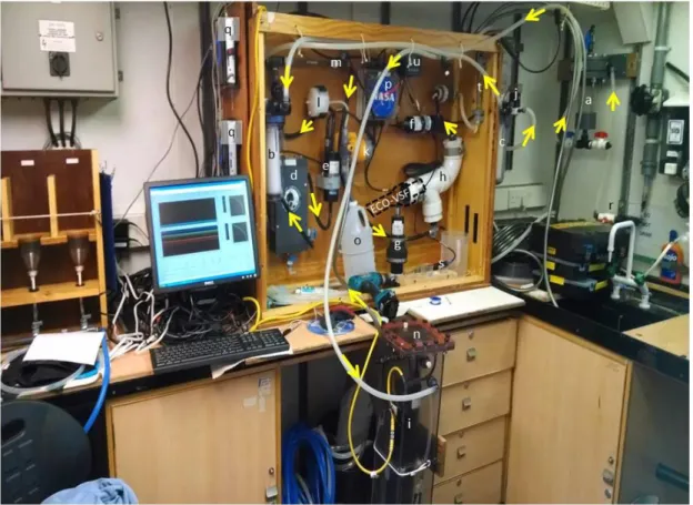
Figure 5. Balch Lab flow-through bio-optical system (shown here being assembled at the beginning of an Atlantic Meridional Transect cruise, so some of the hoses were not yet attached). Arrows denote flow path of science seawater. Letters denote different parts of the system as follows: a) de-bubbler; b) 0.2-m filter canister (only used daily 0.2-m filtered calibration of entire system); c) serially mounted 1 and 0.2-m filter canister (not visible) in ac-9 loop only, upstream of ac-9; d) Sea-Bird thermosalinograph; e) WET Labs chlorophyll fluorometer; f) WET Labs CDOM fluorometer; g) WET Labs ECO-VSF (not yet installed in its flow chamber); h) flow chamber for ECO-VSF made from PVC curved pipe painted flat black inside to minimize internal reflections (dashed line shows orientation of ECO-VSF if installed); i) WET Labs ac- 9; j) solonoid in ac-9 loop to divert seawater through filter manifold upstream of ac-9; k) pump for periodically (programmable for every several minutes) dispensing low volumes of glacial acetic acid into seawater stream to drop the pH and dissolve calcite (calcium carbonate) prior to entering ECO-VSF

(14)

chamber (to measure bbp-a , aka acid-labile backscattering); l) 0.2-m filter for glacial acetic acid stock; m) in-line mixing column to mix seawater and glacial acetic acid; n) ac-9 aquarium; o) glacial acetic acid reservoir; p) junction box for splitting power to different instruments; q) computers to run flow system; r) seawater source; s) pH probe which mounts at point "m" in diagram; t) flow meter in ECO-VSF loop; u) controller for pH probe. Not visible: flow meter in ac-9 loop.

5.6.1 Specialized chambers for backscattering measurements and its characterization An acceptable chamber for optical measurements is one that minimally interferes with the measurement (e.g., measurements in water, Rosette, and in chamber have a small bias between them) and with the chamber effect being characterized (the bias is known so it can be removed).

Instruments should be oriented in the chamber so that settling particles will not accumulate on the instrument’s face and particles are easily flushed into and out of the chamber to avoid particle sorting.

Characterized specialized chambers for backscattering measurements (such as the one used in Dall’Olmo et al. 2009 and seen in Fig. 6) can be custom made or purchased from Sequoia Scientific, Inc. The chambers have a light baffle to limit the possibility that the light from the sensor’s source will be reflected into the sensor’s detector; the sensor has to be oriented such that the line between source and receiver is parallel to the light baffle. The characterization of the wall effect is accomplished by obtaining measurements of scattering after filling the enclosure with high-quality Deionized Water (DIW)¹⁰ with ample time for bubbles to degas (for more details see Dall’Olmo et al. 2009). Values should be minimally different from those expected theoretically (DIW + dark), as the relative contribution of the wall effect will decrease as particulate

concentration increases, and accounting for that is not trivial.

Figure 6. In-line setup of W. Slade in a UNOLS vessel lab. Yellow arrows denote the flow direction.

10By high-quality DIW we mean deionized water that has a resistance of 18.2M and has been radiated with a UV lamp to photo oxidize organics. Also known as ultrapure water or Type I water.

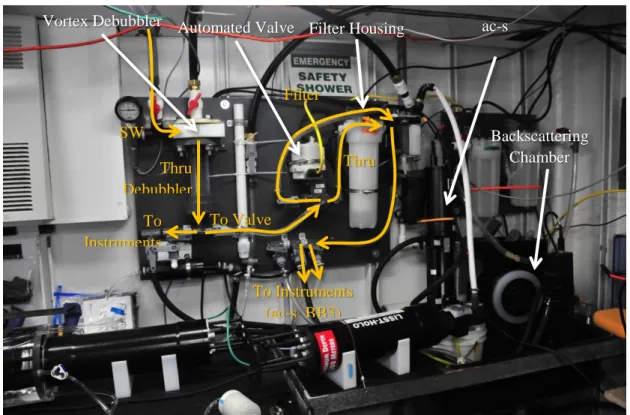
Backscattering Chamber

Vortex Debubbler ac-s

Instrument Automated Valve Filter Housing

SW In

To Instruments

To Valve

Thru Filter Filter

Bypass

Thru Debubbler

To Instruments (ac-s, BB3)

(15)

5.7 Cleaning

Periodic cleaning of all instrumentation is required to remove bacterial films from instrument windows or remove particles that may not get flushed out of the flat-faced instrument enclosure. For typical oligotrophic open-ocean conditions, this weekly instrumental cleaning is sufficient; in meso- and eutrophic conditions, more frequent cleaning is required. Following cleaning, if a significant change (drop) in signal is observed, fouling has likely degraded the previous data, which should be flagged accordingly and corrected, if possible (for example by removing a trend). However, it is still unclear whether it is better to assume a linear trend or an exponential trend, given that fouling organisms typically grow exponentially (Manov et al. 2004).

Refer to manufacturer protocols for cleaning details (e.g., suggested solvents and detergents) for specific sensors. Use lens paper on all optical surfaces (e.g., windows, flow sleeves) to ensure that their properties do not change in time due to scraping with harsher materials. More careful

procedures are warranted when cleaning heavily fouled instruments as optical surfaces can be damaged if grit is scraped across them. More frequent cleaning (e.g., daily) is recommended for the enclosures of flat-faced sensors (such as employed with WET Labs ECO-type sensors) as the slower flow within the chamber sometimes allows for particles to accumulate within the chamber.

5.8 Calibration

Pre- and post-cruise calibration of optical instruments is highly recommended to help establish measurement uncertainty. For example, some optical instruments—in particular, the ac- 9, ac-s, backscattering and transmissometers with 660 nm red LEDs—are known to drift

significantly during a single cruise. If high-quality DIW is available and conditions are adequate, it is recommended to calibrate these instruments throughout the cruise (e.g., Dall’Olmo et al.

2017). Taking discrete water samples to measure CDOM absorption/attenuation on the vessel or back on shore, if following correct protocol, can be used to vicariously calibrate the in-line ac- meter, as long as it is sufficiently close in time (e.g., Matsuoka et al. 2017), to provide hourly CDOM estimates (in this mode the ac-meter, when measuring filtered water, is used to interpolate between the discrete samples).

If calibration is not feasible for ac-meters and transmissometers (i.e., one cannot obtain the signal of DIW at sea), a switching valve can be used to measure “calibration independent”

particulate optical properties as discussed in Section 5.3. This method provides the optical properties of particles using the dissolved fraction as the blank and, if the blanks are measured frequently enough, is not sensitive to slow instrument drift (such as observed for the instruments discussed here). Long-term changes in the measurement done with 0.2-m filtered water can also provide a diagnostic of drift due to instrument fouling. These measurements can be used to correct for the drift (though the best strategy is to clean regularly to avoid the drift due to fouling). Passage of DIW throughout the whole system also provides a means to estimate the enclosure-effect on flat-faced sensors at sea (Section 5.6.1) and fouling within the system. When doing so, attention must be paid to the possibility that large particles may be detached from the plumbing due to the difference in temperature and salinity of the DIW water relative to salt water contaminating the DIW reading.

Dark offsets of flat-faced sensor instruments such as ECO-BB3 and fluorometers should be periodically measured using black electrical tape on the detector—or both detector and source—with the instrument immersed in water (Sullivan et al. 2013). Be sure to remove tape residue with isopropyl alcohol and/or a mild detergent (3M Super 33+ tape is recommended to minimize residues). The difference between the dark measured as part of the in-line system and

(16)

that of the manufacturer may be significant (~10% of signal) in open ocean conditions and hence is important to characterize.

For the LISST we found that the 0.2-m filtered fraction provides a more consistent and lower calibration (termed zscat) than one derived from DIW water (Boss et al. 2018). This is because the salinity-driven change in the index of refraction between window and water can create a significant bias in instruments with a short path-length (Boss et al. 2013b). Since the instrument measures at 670 nm, the contribution of CDOM to the transmission measurement can, in most cases, be neglected.

5.9 Ancillary data

In many instances, optical measurements are used as proxies for biogeochemical parameters (e.g., Chlorophyll a, particulate organic carbon, suspended particulate matter, dissolved organic carbon, pigments, particle size distribution). The proxies are often more valuable to the oceanographic community than the IOPs themselves. While global proxy relationships exist, it is strongly recommended that biogeochemical measurements are made periodically along the cruise to establish the cruise-specific or regional relationships and ensure that the relationships used are consistent with the measurements. Operators must be trained to take discrete samples of water directly from the in-line system to avoid water collection during periods of filtered seawater acquisitions (which will be particle free). Moreover, as the temporal variability in the signal can be important even within five minutes (e.g., changes of one order of magnitude of Chlorophyll a in the North Atlantic while the ship is cruising at 12 knots crossing a front have been observed), an accurate recording of the time of the discrete sample collection is necessary.

5.10 Quality assurance and quality control

To ensure that the in-line system does not bias the measurements, it is critical to make measurements on both in-line as well as surface waters from discrete near-surface Niskin bottle samples and compare measurements from both sources; these may include optical measurements as well as biogeochemical measurements (to check for consistency). In addition, certain

relationships between parameters measured by different instruments are anticipated. For example, transmissometers should agree within a consistent difference due to their design differences (e.g., acceptance angle). Beam-attenuation, backscattering, and chlorophyll are all related in the surface ocean and although they are sensitive to different particle characteristics, robust relationships between them have been derived (e.g., Westberry et al. 2010). In addition, crossing of oceanic fronts is generally observed in both physical and optical measurements. Significant deviations from these relationships may point to a problem in the data. In general, measurements should change slowly with the exception of spikes due to large particles (or bubbles) and front crossings.

Fluctuations in the signal might reveal that bubbles, ambient light, or other unwanted elements are perturbing the observations. Ancillary measurements such as underway system flow rate and pressure, changes in ship’s course or speed, and sea state can also be used to flag regions of data requiring more detailed examination. See the QARTOD manual for a general guide to quality assurance and quality control of optical data.¹¹

6. Acquisition Software, Logging Data

A general recommendation for data logging software is that it should be stable and able to frequently write data to the hard drive of the computer instead of buffering large amounts of

11 https://ioos.noaa.gov/project/qartod/

(17)

data in memory. Small digestible files that are simple to read will ease data processing. For example, for the ac-9 and ac-s instruments, a custom version of Compass (r2.1) was provided by the manufacturer to write hourly files and avoid generating gigabyte-sized files that are difficult to open and process. Note that Compass r2.1 will timestamp files at the beginning or the end of the hour, and depending on how data is recorded, it might significantly slow down a computer.

The last hour of data is kept in memory and may be lost if the software is not stopped properly. It should also be noted that Compass r2.1 does not record instrument internal temperature, which significantly limits the ability to post process internal temperature corrections (e.g., it will use the LUT in the device file, but the output data will be uncorrectable if the wrong device file is used).

How often to write a file is user dependent. Some groups elect to generate 10-minute files to avoid losing more than 10 minutes of data due to any problems. Other optical sensors can be logged with the WET Labs host program (WLHost, with or without their DH-4 data-logger) to record hourly files, or with data from individual instruments connected to their native software using virtual serial ports for real-time data visualization. We do not recommend using the DH4 data logger for extended periods of times (i.e., more than a day) because its internal clock drifts with time and may result in poor timestamping of the data on long expeditions. Terminal software such as TeraTerm (version >1.9.5) may also be used to save data from any serial sensor and timestamp it robustly. However, these programs do not provide a real-time plot of the data. When possible, visualization of the data in real-time will help to monitor the in-line system and

troubleshoot issues as they arise. Sensors can also be logged with the Inlinino hardware/software interface¹², a simple data logger and visualizer built specifically for acquisition of underway system data.

Automated backup, clock synchronization across instruments, and computers used for data logging should be set up at the beginning of the cruise. We recommend logging GPS data directly onto the computer(s) logging instruments and that multiple copies of the data are located at different places on the ship and frequently synchronized (every few hours). Many software options exist to back up data; the laboratory at the University of Maine has had good experiences with SyncToy from Microsoft that is run every four hours using the Windows Task Scheduler.

We recommend that the data logging software saves processed raw ASCII files (in engineering units) and also the raw binary files to the computer (for ac-meters). This is critical in case raw data processing is done incorrectly, e.g., the wrong device file is used for the ac-meters (reinforcing the need to record internal temperature).

7. Considerations for Specific Instruments/Measurements

7.1 Chlorophyll fluorescence and non-photochemical quenching

Phytoplankton decrease their fluorescence within seconds of exposure to high light.

Hence, measurements of chlorophyll fluorescence depend on the short-term light-acclimation state of the phytoplankton, which are affected in turn by the residence time of the water within the dark plumbing system, clear tubing, or within an illuminating instrument. Differences between day and night as well as effects of lights within the ship/lab may occur and may be corrected.

Ensuring that the tubing is dark or covered with electrical tape will help with non-photochemical quenching inside the ship. However, a downside to using dark tubes is that biofouling of the lines cannot be visualized.

12 http://inlinino.readthedocs.io/

(18)

7.2 Chlorophyll fluorescence measurement and CDOM

Fluorescence by CDOM, if significant in the water, contaminates the measurements by chlorophyll fluorometers (e.g., Proctor and Roesler 2010). To assess this problem, we recommend periodically measuring the seawater that has passed through a 0.2-m filter to create a baseline (see Sections 5.3 and 5.8 on in-line filters and calibration).

7.3 Absorption and attenuation

Instruments commonly used to measure absorption and attenuation in ocean optics are designed for in situ deployment but they can be adapted to underway systems: the WET Labs ac-s and ac-9, and C-Star are built with flow cells, and the Sequoia Scientific, Inc. LISST-100X has a flow chamber accessory that allows for flow-through measurements. As previously indicated, regular calibrations (about once per year) of the ac-meter by the manufacturer are important for the stability of the collected data. After the manufacturer’s calibration, a new device file recording the electronic responses of the ac-meter to instrument temperature will be generated.

Always back up all device files and use the latest device file for new data collection.

Calibration is important for obtaining quality measurements; if particulate measurements are primarily of interest, periodic filtration with a 0.2-m filter can be used to provide

“calibration independent” particulate measurements by difference of total and dissolved measurements. This is particularly important when the calibration (and other instrumental) uncertainties become a significant part of the signal. For example, the LISST-100X and LISST- 200X, which have short pathlengths (5 or 2.5 cm), are less sensitive in very clear water (meaning calibration uncertainties become a large part of the signal (Slade et al. 2010). If dissolved or total absorption and attenuation are of interest, at least a daily pass of DIW through the system

(Dall’Olmo et al. 2017), or a daily sample of CDOM absorption (Matsuoka et al. 2017), is required. Annual calibration by the manufacturer is necessary for ac-9 and ac-s instruments as it provides an updated look-up table (which is part of the device file) that will compensate for instrument drift due to the instrument’s temperature changes. It is critical that this table matches temperatures that are likely to be found in the environment in which the sensor is deployed (always request an “extended” table if you plan to work in tropical or polar regions).

8. Processing Flow-Through Data

The processing of flow-through data consists of five steps that should be executed in the following order:

1. Synchronization

2. Separating the data into periods where different water goes through the system (DIW, filtered seawater (FSW), and total seawater (TSW), referred to below as “period type”)

3. Binning

4. Interpolation (DIW on FSW and FSW on TSW) 5. Instrument specific calibration and corrections

The synchronization should be run first to ensure that the separation by period type is similar for all optical instruments using periods where water is passed through the 0.2-m filter for calibration of particulate properties, and if calibration of instruments requires data from other instruments (e.g., temperature or FDOM). When binning the data, it is important to properly separate them by period types to avoid a bin that includes the average of both the FSW and TSW

(19)

periods, which would result in an unusable bin. Links to software that performs these tasks are in Appendix III.

8.1 Synchronizing

Quantifying the lags between instruments (if significant) is important when merging data from multiple sensors. This may be more important for some measurements, such as temperature and salinity correction of absorption. Generally, it is advisable to merge prior to processing. This enables the comparison of related parameters (e.g., absorption and fluorescence of CDOM and/or chlorophyll) for quick quality control to ensure that the specific time delays applied are correct (crossing of an optical front in one instrument’s output coincides with the other). Feature tracking (e.g., crossing fronts) will help synchronize the instruments for each sensor to ensure accurate merging. It is also possible to introduce a dye solution to test that the merging is done correctly.

Periods with a strong change in flow rate must be revisited as the synchronization between instruments could be affected.

8.2 Separating data into period types

Separating data into period types is a critical step of the processing for instruments that require periodic calibration. When the system switches between two types of measurements (e.g., TSW to FSW), the residence time of each instrument must be considered and the short period of measurements following the switching event should be discarded. Commercial systems that automate the periodic FSW measurements also record their valve position which allows automation of this step.

8.3 Binning

The high temporal resolution of in-line data allows one to bin the data, a process that increases signal-to-noise ratio. Using a median bin, or a specific percentile, helps reduce

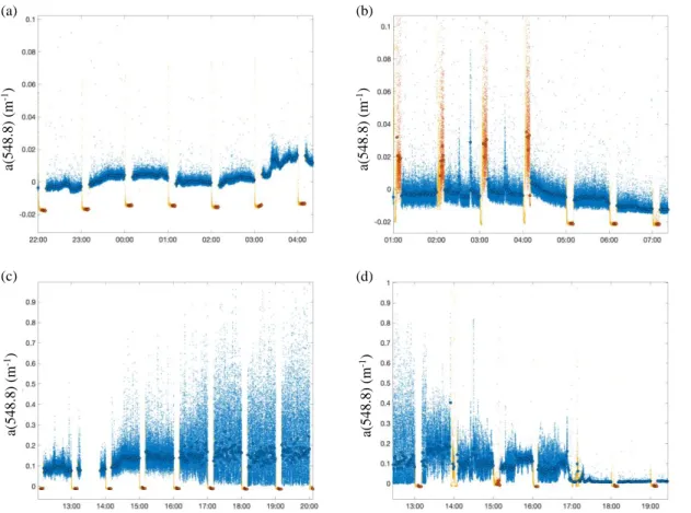
contamination by spikes due to bubbles or rare large particles (first section of Fig. 7c). The longer the bin, the more smeared the resulting spatial signal, hence we do not advise binning beyond one minute (providing a spatial scale of ~300 m for a vessel moving at 10 knots), unless increased signal/noise is required and the lower spatial resolution is acceptable.

8.4 Removal of data contaminated by bubbles

Periods with enhanced bubble contamination are easy to visualize and must be removed from the data. These periods are characterized by an abrupt increase in variance and “spiky” data, and should be flagged or discarded (Fig. 7b, c, d). Note that zooplankton trapped in the

backscattering casket (BB-box) can cause similar contamination (Burt and Tortell 2018). An automated technique that works well to quality check ac-s spectra is to compute chlorophyll a from the absorption line height (e.g., Boss et al. 2013a). If the values obtained are unrealistic (negative, or above 100 μg L^-1) both particulate absorption and attenuation spectra are flagged.

While this is a helpful method, data should still be manually validated for unexpected features.

(20)

Figure 7. Example time series of absorption at 548.8 nm measured by an ac-s in the North Atlantic. Small dots correspond to raw data while larger dots correspond to minute-binned observations. Blue symbols are total seawater (TSW) measurements, red symbols are filtered seawater (FSW) measurements, and yellow symbols correspond to discarded data. a) shows a section of “acceptable” measurements; b) shows a time series with bubbles during the FSW measurements; c) and d) show a time period with high noise likely due to bubbles or very large particles. Note that for all bins the several statistical parametric and non-

parameteric quantities are computed (median, mean, standard deviation, and 16^th and 84^th percentiles) and are used to assign spectra uncertainties submitted to SeaBASS.

8.5 Interpolating

When using periodic calibrations and/or filtered periods for particulate measurements, it is important to view all values between subsequent cleaning to assess their consistency and remove obvious outliers (e.g., large change in values not associated with fronts or change in total measurements). It is recommended to linearly interpolate in between “good” blanks rather than use the preceding blank, the following blank, or the average of the blanks. If the system is cleaned in between two blanks and the method recommended above does not work, we suggest discarding any data within that period (typically less than 30 minutes). To prevent discarding data, always start and finish the acquisition of data with a blank. This is especially true for instruments (e.g., ac-s) that drift quickly with time.

(a)

(c) (d)

(b)

a(548.8) (m-1) a(548.8) (m-1)a(548.8) (m-1)

a(548.8) (m-1)

(21)

8.6 Instrument specific calibration and corrections

8.6.1 ac-meters

The mismatch in spectral band positions between absorption and attenuation are

corrected using interpolation. For the ac-s in clear open ocean waters, the third method described in Zaneveld et al. (1994) is recommended to correct for scattering using 730 nm as the null wavelength while simultaneously performing a residual temperature correction (Slade et al.

2010). Other methods for scattering correction also exist (e.g., Röttgers et al. 2013) which may be more appropriate in coastal waters and where significant amounts of non-algal particles are present. Attenuation can also be corrected for residual temperature effects. A spectral unsmoothing based on the method in Chase et al. (2013) may be applied to sharpen spectral features. The resulting spectra may exhibit negative absorption values in the blue regions, but these values are not significantly different from zero. Note that it is critical to send the ac-meter sensor to the manufacturer on an annual basis even when using the “calibration independent”

method to ensure that the look-up table to correct the instrument-temperature-effect in the device file is current.

8.6.2 Eco-BB3

The particulate volume scattering function (VSF) is obtained by subtracting the filtered values from the total values (filtered values are linearly interpolated). The dissolved VSF is obtained by subtracting the DIW measurements from filtered measurements (interpolating in time between successive daily DIW values). Those differences compensate for the dark and wall effects of the BB-box. A temperature and salinity correction is performed on the dissolved portion of the backscatter using Zhang et al. (2009). The particulate backscattering coefficient (bbp) is computed using a χ factor from Sullivan et al. (2013).

8.6.3 LISST

The LISST measurements are processed using procedures described in Boss et al. (2018), Agrawal and Pottsmith (2000), and the Sequoia Scientific, Inc. Processing Manual (2008).

(22)

References

Agrawal, Y. C. and H.C. Pottsmith, 2000: Instruments for particle size and settling velocity observations in sediment transport. Mar. Geol. 168: 89–114.

Balch, W., D. Drapeau, B. Bowler, E. Booth, J. Goes, A. Ashe, and J. Frye, 2004: A multi-year record of hydrographic and bio-optical properties in the Gulf of Maine: I. Spatial and temporal variability. Prog. Oceanogr., 63: 57–98. doi:10.1016/j.pocean.2004.09.003 Boss, E., M. Picheral, T. Leeuw, A. Chase, E. Karsenti, G. Gorsky, L. Taylor, W. Slade, J. Ras,

and H. Claustre, 2013a: The characteristics of particulate absorption, scattering and attenuation coefficients in the surface ocean; Contribution of the Tara Oceans expedition.

Methods in Oceanography, 7: 52–62. doi:10.1016/j.mio.2013.11.002

Boss, E., H. Gildor, W. Slade, L. Sokoletsky, A. Oren, and J. Loftin, 2013b: Optical properties of the Dead Sea. Journal of Geophysical Research, 118: 1821–1829.

doi:10.1002/jgrc.20109

Boss, E., N. Haentjens, T. K. Westberry, L. Karp-Boss, and W. Slade, 2018: Validation of the particle size distribution obtained with the laser in-situ scattering and transmission (LISST) meter in flow-through mode. Optics Express, 26(9): 11125–11136.

doi:10.1364/OE.26.011125

Burt, W. J., and P.D. Tortell, 2018: Observations of zooplankton diel vertical migration from high-resolution surface ocean optical measurements. Geophysical Research Letters, 45.

doi:10.1029/2018GL079992

Cetinic, I., M.J. Perry, N. T. Briggs, E. Kallin, E.A. D’Asaro, and C.M. Lee, 2012: Particulate organic carbon and inherent optical properties during 2008 North Atlantic bloom

experiment. Journal of Geophys. Res. Oceans, 117: C06028. doi:10.1029/2011JC007771 Cetinic, I., N. Poulton and W. Slade, 2016: Characterizing the phytoplankton soup: pump and

plumbing effects on the particle assemblage in underway optical seawater systems.

Optics Express, 24(18): 20703-20715. doi:10.1364/OE.24.020703

Chase, A., E. Boss, R. Zaneveld, A. Bricaud, H. Claustre, J. Ras, G. Dall’Olmo, and T. K.

Westberry, 2013: Decomposition of in situ particulate absorption spectra. Methods in Oceanography. doi:10.1016/j.mio.2014.02.002

Dall’Olmo, G., T.K. Westberry, M.J. Behrenfeld, E. Boss, and W.H. Slade, 2009: Significant contribution of large particles to optical backscattering in the open ocean.

Biogeosciences, 6: 947–967.

Dall’Olmo G., R. J. W. Brewin, F. Nencioli, E. Organelli, I. Lefering, D. McKee, R. Röttgers, C.

Mitchell, E. Boss, A. Bricaud, and G. Tilstone, 2017: Determination of the absorption coefficient of chromophoric dissolved organic matter from underway spectrophotometry.

Optics Express, 25(24): A1079-A1095. doi:10.1364/OE.25.0A1079

Graff, J. R., T.K. Westberry, A.J. Milligan, M.B. Brown, G. Dall’Olmo, and V. van Dongen- Vogels, et al. 2015: Analytical phytoplankton carbon measurements spanning diverse

(23)

ecosystems. Deep Sea Res. Part I: Oceanogr. Res. Pap. 102: 16–25.

doi:10.1016/j.dsr.2015.04.006

Henin, C. and J. Grelet, 1996: A merchant ship thermosalinograph network in the Pacific Ocean.

Deep Sea Res., 11-12: 1833–1856.

Juranek, L. W., R. C. Hamme, J. Kaiser, R. Wanninkhof, and P. D. Quay, 2010. Evidence of O2 consumption in underway seawater lines: Implications for air-sea O2 and CO2 fluxes.

Geophys. Res. Lett., 37: L01601. doi:10.1029/2009GL040423

Liu, Y., Boss, E., Chase, A., Xi, H., Zhang, X., Röttgers, R., Pan, Y., Bracher, A. 2019: Retrieval of phytoplankton pigments from underway spectrophotometry in the Fram Strait. Remote Sensing, 11(3): 318.

Liu, Y., R. Röttgers, M. Ramírez-Pérez, T. Dinter, F. Steinmetz, E.M. Nöthig, S. Hellmann, S.

Wiegmann, and A. Bracher, 2018: Underway spectrophotometry in the Fram Strait (European Arctic Ocean): a highly resolved chlorophyll a data source for complementing satellite ocean color. Optics Express, 26(14): A678–A696. doi:10.1364/OE.26.00A678 Lorenzen, C.J., 1966: A method for the continuous measurement of the in vivo chlorophyll

concentration. Deep Sea Res. 13: 223–227.

Manov, D. V, G.C. Chang, and T.D. Dickey, 2004: Methods for reducing biofouling of moored optical sensors. Journal of Atmospheric and Oceanic Technology, 21: 958–969.

Matsuoka, A., E. Boss, M. Babin, L. Karp-Boss, M. Hafez, A. Chekalyuk, C. W. Proctor, P. J.

Werdell, and A. Bricaud, 2017: Pan-Arctic optical characteristics of colored dissolved organic matter: Tracing dissolved organic carbon in changing Arctic waters using satellite ocean color data. Remote Sensing of Environment, 200: 89–101.

doi:10.1016/j.rse.2017.08.009

Proctor, C. W. and C. S. Roesler, 2010: New insights on obtaining phytoplankton concentration and composition from in situ multispectral Chlorophyll fluorescence. Limnol. Oceanogr.

Methods, 8: 695–708. doi:10.4319/lom.2010.8.695

Röttgers, R., D. McKee, B. Sławomir, and S. Woźniak, 2013: Evaluation of scatter corrections for ac-9 absorption measurements in coastal waters. Methods in Oceanography, 7: 21–39.

doi:10.1016/j.mio.2013.11.001

Slade, W. H., E. Boss, G. Dall’Olmo, M.R. Langner, J. Loftin, M.J. Behrenfeld, and T.K.

Westberry, 2010: Underway and Moored Methods for Improving Accuracy in

Measurement of Spectral Particulate Absorption and Attenuation. Journal of Atmospheric and Oceanic Technology, 27(10): 1733–1746. doi:10.1175/2010JTECHO755.1

Sullivan J.M., M.S. Twardowski, J. Ronald, V. Zaneveld, and C. Moore, 2013: Measuring optical backscattering in water. In: Light Scattering Reviews 7. Springer Praxis Books. Springer, Berlin, Heidelberg. 189–224. doi:10.1007/978-3-642-21907-8_6

Werdell, J. P., C. W. Proctor, E. Boss, T. Leeuw, and M. Ouhssain, 2013: Underway sampling of marine inherent optical properties on the Tara Oceans expedition as a novel resource for

(24)

ocean color satellite data product validation. Methods in Oceanography, 7: 40–51.

doi:10.1016/j.mio.2013.09.001

Westberry, T.K, G. Dall'Olmo, E. Boss, M.J. Behrenfeld, and T. Moutin, 2010. Coherence of particulate beam attenuation and backscattering coefficients in diverse open ocean environments. Opt. Express, 18(15): 15419–15425. doi:10.1016/j.mio.2013.09.001 Zaneveld J., R. V., J. Kitchen, and C. Moore, 1994: Scattering error correction of reflecting tube

absorption meter. Ocean Optics XII. SPIE Proceedings, 2258: 44–55.

doi:10.1117/12.190095

Zhang, X., L. Hu, and M.‐ X. He, 2009: Scattering by pure seawater: Effect of salinity. Opt.

Express, 17(7): 5698– 5710.

(25)

Appendix I: Pre-Cruise Checklist

 Contact the ship regarding pump and cleaning of in-line pipes.

 Contact the ship regarding adequate DIW source (UV lamp, 18.2Msufficient quantity

and replacement filters for it.

 Contact ship regarding possibility to visit or get pictures of the lab and sink where you will install your system. Know in advance how you will connect to the intake pump and bring several possible adapters.

 Make sure the ship’s personnel know how much water (from instruments and debubbler) will go into the sink; some sinks empty directly into the sea and some empty into a hold.

 Check about access to GPS data for your logging computer (typically a serial or Ethernet feed).

 Check that all instruments and cables are packed—including spares. Bring spare power supplies, serial to USB converters, and required drivers. Plan for each electronic element to be splashed with seawater; think about what might need to be replaced.

 Check that you have sufficient filters to last the whole expedition (pack for extras in case you encounter productive waters).

 Sufficient tubing and replacement tubing. Hose clamps, connectors, valves.

 Tool box.

 Cleaning supplies: detergent, isopropyl alcohol, optical wipes, sponges.

Appendix II: At-Sea Checklist

Throughout the day:

 Note logged flow rate and compare to previous day (ideally 3 to 5 L/min).

 Look for bubbles by viewing the output of the ac-s and ECO-bb sensors and noticing the variance in the signal (in ac-s bubbles will result in noticeable disruption in the middle of the spectra).

 Make sure filtration periods occur when scheduled and are long enough for value to stabilize. If high variability area such as costal water, increase frequency of filtered periods (e.g., every 30 minutes instead of every hour).

 Check that data are backed up.

 Check that all software is recording data.

 Check date and time of computer (must be UTC).

 Check power supply (e.g., 12–13.5 V for ac-s, LISST, ECO).

 If using Compass r2.1 to log data, check that the number of records lost on Compass r2.1 is not too high (<20). If it is, reboot software. Consider defragmenting hard drive and restarting logging computer.

Once a day:

 Clean casket for backscatter measurements and LISST flow cell.

 Run DIW through the whole system until all instruments attain steady-state values.

Record at least one minute of these conditions.

 Analyze some data to verity data acquired is reasonable.

Weekly (more frequent in eutrophic waters or if you notice a significant jump in the data following the cleaning):

 Clean ac-s.

 Replace 0.2-m filter.

(26)

 Once the filter is replaced, run the system switching back and forth between filtered and unfiltered mode until bubbles no longer enter the system from the filter housing (this can be accelerated using the purging valve in the filter housing).

Appendix III: Processing Software for AC-Meters in Flow-Through

The University of Maine group has posted several processing codes for in-line optical data in the public domain:

1. https://github.com/OceanOptics/ACCode 2. https://github.com/OceanOptics/InLineAnalysis

These codes contain processing, QC modules, and modules to generate SeaBASS files.

The Alfred Wegner Institute Phytooptics group has posted processing codes for in-line ac-s data in the public domain: https://github.com/phytooptics/acs_flowthrough

IOCCG Ocean Optics and Biogeochemistry Protocols for Satellite Ocean Colour Sensor Validation