Article
Field Intercomparison of Radiometer Measurements for Ocean Colour Validation
Gavin Tilstone1,*, Giorgio Dall’Olmo1,2 , Martin Hieronymi3 , Kevin Ruddick4,
Matthew Beck4 , Martin Ligi5, Maycira Costa6, Davide D’Alimonte7, Vincenzo Vellucci8 , Dieter Vansteenwegen9, Astrid Bracher10 , Sonja Wiegmann10, Joel Kuusk5 ,
Viktor Vabson5 , Ilmar Ansko5, Riho Vendt5 , Craig Donlon11and Tânia Casal11
1 Plymouth Marine Laboratory, Earth Observation Science and Applications, Plymouth PL1 3DH, UK;
gdal@pml.ac.uk
2 National Centre for Earth Observations, Plymouth PL1 3DH, UK
3 Institute of Coastal Research, Helmholtz-Zentrum Geesthacht (HZG), 21502 Geesthacht, Germany;
martin.hieronymi@hzg.de
4 Royal Belgian Institute of Natural Sciences, 29 Rue Vautierstraat, 1000 Brussels, Belgium;
kruddick@naturalsciences.be (K.R.); mbeck@naturalsciences.be (M.B.)
5 Tartu Observatory, University of Tartu, 61602 Tõravere, Estonia; martin.ligi@ut.ee (M.L.);
joel.kuusk@ut.ee (J.K.); viktor.vabson@ut.ee (V.V.); ilmar.ansko@ut.ee (I.A.); riho.vendt@ut.ee (R.V.)
6 Geography Department at the University of Victoria, Victoria, BC V8P 5C2, Canada; maycira@uvic.ca
7 Center for Marine and Environmental Research CIMA, University of Algarve, 8005-139 Faro, Portugal;
davide.dalimonte@aequora.org
8 Sorbonne Université, CNRS, Institut de la Mer de Villefranche, IMEV, F-06230 Villefranche-sur-Mer, France;
enzo@imev-mer.fr
9 Flanders Marine Institute (VLIZ), Wandelaarkaai 7, 8400 Ostend, Belgium; dieter.vansteenwegen@vliz.be
10 Alfred Wegener Institute Helmholtz Centre for Polar and Marine Research, Department of Climate Sciences, D-27570 Bremerhaven, Germany; Astrid.Bracher@awi.de (A.B.); Sonja.Wiegmann@awi.de (S.W.)
11 European Space Agency, 2201 AZ Noordwijk, The Netherlands; craig.donlon@esa.int (C.D.);
tania.casal@esa.int (T.C.)
* Correspondence: ghti@pml.ac.uk; Tel.:+44-1752-633-406
Received: 31 March 2020; Accepted: 11 May 2020; Published: 16 May 2020
Abstract:A field intercomparison was conducted at the Acqua Alta Oceanographic Tower (AAOT) in the northern Adriatic Sea, from 9 to 19 July 2018 to assess differences in the accuracy of in- and above-water radiometer measurements used for the validation of ocean colour products.
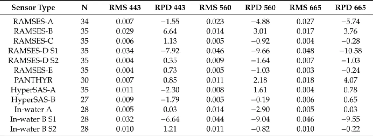
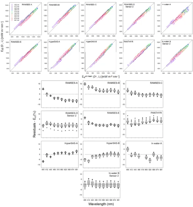
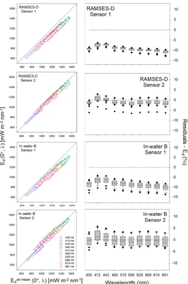
Ten measurement systems were compared. Prior to the intercomparison, the absolute radiometric calibration of all sensors was carried out using the same standards and methods at the same reference laboratory. Measurements were performed under clear sky conditions, relatively low sun zenith angles, moderately low sea state and on the same deployment platform and frame (except in-water systems). The weighted average of five above-water measurements was used as baseline reference for comparisons. For downwelling irradiance (Ed), there was generally good agreement between sensors with differences of<6% for most of the sensors over the spectral range 400 nm–665 nm. One sensor exhibited a systematic bias, of up to 11%, due to poor cosine response. For sky radiance (Lsky) the spectrally averaged difference between optical systems was<2.5% with a root mean square error (RMS)<0.01 mWm−2nm−1sr−1. For total above-water upwelling radiance (Lt), the difference was
<3.5% with an RMS<0.009 mWm−2nm−1sr−1. For remote-sensing reflectance (Rrs), the differences
between above-water TriOS RAMSES were<3.5% and<2.5% at 443 and 560 nm, respectively, and were
<7.5% for some systems at 665 nm. Seabird-Hyperspectral Surface Acquisition System (HyperSAS) sensors were on average within 3.5% at 443 nm, 1% at 560 nm, and 3% at 665 nm. The differences between the weighted mean of the above-water and in-water systems was<15.8% across visible bands. A sensitivity analysis showed thatEdaccounted for the largest fraction of the variance in Rrs, which suggests that minimizing the errors arising from this measurement is the most important
Remote Sens.2020,12, 1587; doi:10.3390/rs12101587 www.mdpi.com/journal/remotesensing
Remote Sens.2020,12, 1587 2 of 48
variable in reducing the inter-group differences inRrs. The differences may also be due, in part, to using five of the above-water systems as a reference. To avoid this, in situ normalized water-leaving radiance (Lwn) was therefore compared to AERONET-OC SeaPRiSMLwnas an alternative reference measurement. For the TriOS-RAMSES and Seabird-HyperSAS sensors the differences were similar across the visible spectra with 4.7% and 4.9%, respectively. The difference between SeaPRiSMLwn
and two in-water systems at blue, green and red bands was 11.8%. This was partly due to temporal and spatial differences in sampling between the in-water and above-water systems and possibly due to uncertainties in instrument self-shading for one of the in-water measurements.
Keywords: fiducial reference measurements; remote sensing reflectance; ocean colour radiometers; TriOS RAMSES; Seabird HyperSAS; field intercomparison; AERONET-OC; Acqua Alta Oceanographic Tower
1. Introduction
Fiducial reference measurements (FRM) are an important component of satellite missions for the validation of remote sensing products and are used to ensure that the most accurate data are distributed to the user community. FRMs are distinct from other in situ measurements in that they use protocols recommended by international ocean colour organizations and space agencies, are traceable to SI (Système international) units, are referenced to inter-comparison exercises and have a full uncertainty budget [1] to provide independent, high quality validation measurements for the duration of a satellite mission [2,3]. To underpin the validation of satellite ocean colour radiometry, it is therefore essential that radiometers used to collect FRMs are inter-compared to assess data consistency and characterise the potential differences between instruments and methods. In the absence of such intercomparisons, the traceability chain and uncertainty budget are not validated. The use of a wide range of instruments, methods and laboratory practices may only add to the uncertainty of satellite ocean colour products.
The primary data product in satellite ocean colour is remote-sensing reflectance,Rrs. Radiometric field measurements used to derive this parameter are generally obtained from in-water and above-water optical measurements. These include above-water radiometry, underwater profiling, underwater measurements at fixed depths or combined above and underwater measurements from floating systems.
Within the numerous measurement systems that exist, differences in calibration sources, methods and data processing schemes lead to the greatest variation between them [1,4]. To minimise these, best practices on each of the steps used to generate radiometric FRM have been established previously and in this project [5–8].
Since the launch of the Sea-Viewing Wide Field-of-View Sensor (SeaWiFS) in 1997, a growing body of literature on intercomparisons between radiometers has developed, which were conducted to constrain the differences between in-water and satellite ocean colour parameters [9–17]. The National Aeronautics and Space Administration (NASA) SeaWiFS Intercalibration Round Robin Experiments (SIRREX) 1–8 focused on sensor calibration; specifically spectral radiance response using plaques and portable field sources for monitoring the stability of sensors [9–15]. The experiments established protocols for these, which reduced the uncertainties in measurements from 8% to 1%. During SIRREX 5, comparisons between in-water radiometers were conducted at Little Seneca Lake in Maryland, USA and comparisons of above-water radiometers were conducted in the laboratory [11]. Differences in in-water apparent optical properties were found to be related to the stability of the platform and illumination geometry. For the laboratory comparisons, systematic differences between radiometers were associated with the derivation of the downwelling irradiance from the reflected plaque radiance and smaller differences due to isolated problems with the radiometers. These were addressed in SIRREX 8 through the publication of new laboratory methods for characterising irradiance sensors [15].
Then followed the NASA Sensor Intercomparison and Merger for Biological and Interdisciplinary
Studies (SIMBIOS) Radiometric Intercomparison (SIMRIC) -1 and -2 [12,13]. The purpose of these experiments was to establish a common radiometric scale among the facilities that calibrate in situ radiometers used for ocean colour related research. The final result was an updated document on calibration procedures and protocols [9]. Using these protocols during SIMRIC-2, the SeaWiFS Transfer Radiometer (SXR-II) measured the calibration radiances at six wavelengths from 411 nm to 777 nm, which was compared against measurements from 10 other laboratories [13]. The agreement between laboratories was within the combined uncertainties for all but two laboratories and the errors for these laboratories were traced back to the sensor calibrations. Following the launch of the Medium Resolution Imaging Spectrometer (MERIS) in 2002, the MERIS and Advanced Along-Track Scanning Radiometer (AATSR) Validation Team (MAVT) conducted a series of intercomparison exercises (PlymCal 1-3 [14]) to compare above- and in- water radiometry (Bio-spherical, PR650, SATLANTIC, SIMBADA, SPMR, TACCS and TRIOS). The expected calibration of radiometric sensors is that they are within±1 to 2% of each other and during these intercomparisons this was achieved, except for one sensor that exhibited degradation of the cosine collector. The MERIS Validation Team (MVT) then conducted a field campaign at a coastal site offSouth West Portugal and determined the accuracy of atmospheric and in-water measurements using a hyperspectral, SATLANTIC buoy radiometer with a tethered irradiance chain (TACCS), as well as band-pass filter radiometer of the same design [15]. The overall error for the TACCS system in these waters was 5% where the in-water attenuation coefficient (Kd) was known and 7% whereKdwas modelled and extrapolated from the surface to depth. Under the Assessment of In Situ Radiometric Capabilities for Coastal Water Remote Sensing Applications (ARC) MERIS MVT intercomparison of above-water radiometers (SeaPRISM and RAMSES) and in-water radiometers (WiSPER-Wire-Stabilized Profiling Environmental Radiometer and TACCS) was performed under near ideal deployment conditions at the Acqua Alta Oceanographic Tower (AAOT) in the northern Adriatic Sea [17]. For this intercomparison, all sensors were inter-calibrated through absolute radiometric calibration with the same standards and methods. The spectral water-leaving radiance (Lw), as well asEdandRrswere compared. The relative difference inRrswas between−1% and+6%.
The spectrally averaged values of absolute difference were 6% for the above-water systems and 9% for the in-water systems. The good agreement between sensors was achievable because of the stability of the deployment platform used. The first in situ radiometer intercomparison exercise in support of the Ocean and Land Colour Instrument (OLCI) on-board the Sentinel-3 satellite was conducted at a lake in Estonia in May 2017 under non-homogeneous environmental conditions [4]. It highlighted that there was a large variability between recently calibrated sensors, due to high spectral and spatial variability in the targets and environmental conditions. For the radiance sensors tested, variation in the fields of view (FOV) contributed to the differences whereas for the irradiance sensors, this arose from imperfect cosine response. Following the success of ARC MERIS MVT, and because the environmental conditions are nearly ideal during summer, the AAOT was chosen to undertake the intercomparison reported here.
The main difference over the previous intercomparisons at the AAOT was that: (1) more measurement systems were compared (10 in this study, five in [17]); (2) Seabird HyperSAS and C-OPS were included in this study, whereas in [17] two TACCS systems were included; (3) in this study the above-water sensors were located side by side on purpose-built frames, which ensured that all above-water optical systems pointed at the same patch of water or sky; (4) in [17] the measurements were referenced to in-water WiSPER, whereas in this study they were referenced to the weighted mean of RAMSES and HyperSAS systems and SeaPRISM. The difference from [4], is that in summer the AAOT experiences near-ideal homogeneous conditions for conducting such intercomparisons. The main aim of the AAOT intercomparison was to quantify differences in radiometric quantities determined using a range of above-water and in-water radiometric systems (including both different instruments and processing protocols). Specifically, we evaluated the differences among:
1. Hyperspectral (five above-water TriOS-RAMSES, two Seabird-HyperSAS, one Pan-and-Tilt System with TriOS-RAMSES sensors (PANTHYR), one in-water TriOS-RAMSES system) and multispectral (one in-water Biospherical-C-OPS) sensors.
Remote Sens.2020,12, 1587 4 of 48
2. In-water and above-water measurement systems.
2. Materials and Methods
2.1. Determination of Water-Leaving Radiance: Above-Water
Above-water methods generally rely on measurements of (i.) total radiance from above the seaLt(θ,θ0,∆φ,λ), that includes water-leaving radiance as well as sky and sun glint contributions;
and (ii.) the sky radiance that would be specularly reflected towards theLtsensor if the sea surface was flatLsky(θ0,θ0,∆φ,λ). The measurement geometry is defined by the sea viewing zenith angleθ, the sky viewing zenith angleθ0, and the relative azimuth angle between the sun (φ0) and sensors (φ)
∆φ=φ0−φ[18–21]. Illumination is largely defined by the sun zenith angleθ0, and to a lesser extent atmospheric properties (assuming no clouds). The water-leaving radiance was computed by removing sky glint effects fromLtas follows:
Lw(θ,θ0,∆φ,λ) =Lt(θ,θ0,∆φ,λ)−ρ(θ,θ0,∆φ,U10)Lsky(θ0,θ0,∆φ,λ), (1) whereρ(θ,θ0,∆φ,U10)is an estimate of the sea surface reflectance typically expressed as a function of the sun-sensor geometry and of the wind speed 10 m above the sea surface,U10[18].
2.2. Determination of Water-Leaving Radiance: In-Water
In-water methods to estimate water-leaving radiance require the measurement of the nadir upwelling radiance,Lu(z,λ), or upwelling irradiance,Eu(z,λ), as a continuous profile in the water column or at several fixed depths. The first type of measurement is generally performed with free-fall profilers deployed from a ship [22] or autonomous profiling floats [23]. The second type of measurement is generally performed with optical moorings [24], surface buoys [12] or when instruments have to be lowered manually in the water column [25] from a variety of platforms. Each method has its pros and cons, however all of them have a few principles in common to improve the accuracy of estimatingLw. These include a sufficient number of vertical or temporal measurements to reduce the effect of wave focusing, minimize the effect of instrument self-shading, platform shading and reflection, so that the measurements can also be made as close as possible to the surface and at nadir view.Luis then used to extrapolate the radiometric quantities to just below the water surface (0−) since this cannot be directly measured due to wave perturbations. Although linear extrapolation of log transformed radiometric quantities is the most commonly used technique, this is not always an ideal approach depending on the type of measurements, environmental conditions and wavelength. Finally, theLu(0−,λ)is projected above water to obtain the water-leaving radiance:
Lw=Lu(0−,λ)·(1−ρ0)
n2 , (2)
whereρ0is the water-air interface Fresnel reflection coefficient andnis the refractive index of seawater.
2.3. Determination of Remote-Sensing Reflectance and Normalized Water-Leaving Radiance
The remote-sensing reflectanceRrs(θ,θ0,∆φ,λ)is defined as the ratio of theLwto the above-water downwelling irradianceEd(0+,λ)and was computed as:
Rrs(θ,θ0,∆φ,λ) = Lw(θ,θ0,∆φ,λ)
Ed(0+,λ) . (3)
The exact normalized water-leaving radiance was computed as per [26]:
Lwn(λ) =Rrs(θ,θ0,∆φ,λ)BRDF(θ,θ0,∆φ,λ,chl)F0(λ), (4)
whereF0(λ)is the extraterrestrial solar irradiance [27] and the bidirectional reflectance distribution function (BRDF) factorBRDF(θ,θ0,∆φ,λ,chl)normalizesRrsto a standard geometry (θ=θ0=0):
BRDF(θ,θ0,∆φ,λ,chl) = <(U10)
<(θ,U10)
f0(λ,chl) Q0(λ,chl)
"
f(θ0,λ,chl) Q(θ,θ0,∆φ,λ,chl)
#−1
. (5)
In (5), <(θ,U10) accounts for the reflection-transmission properties of the air-sea interface during the measurement. The term <<((Uθ,U10)
10) and Q remove from Rrs [28] the variability due to viewing angle. The term Q(θ,θf(θ0,λ,chl)
0,∆φ,λ,chl) describes the bi-directionality of the upwelling light field from the ocean, and the corresponding term Qf0(λ,chl)
0(λ,chl) [28] normalizes it to the standard geometry.
Look-up-tables ofQf and<values were computed by [28] for selected wavelengths and were obtained fromftp://oceane.obs-vlfr.fr/pub/gentili/DISTRIB_fQ_with_Raman.tar.gz. The values ofchlrequired for such a correction were obtained from daily averaged total chlorophyll-a high-performance liquid chromatography (HPLC) measurements [29].
2.4. Simulation of Ocean and Land Colour Instrument (OLCI) Bands
Hyperspectral measurements ofLt,Lsky,EdandRrswere converted into equivalent OLCI bands by applying the OLCI spectral response functions [30] as in the following example forLt:
Lt(λi,OLCI) =
R Si,OLCI(λ)Lt(λ)dλ
R Si,OLCI(λ)dλ , (6)
whereLt(λi,OLCI)andSi,OLCI(λ)areLtand the OLCI spectral response function (SRF) for theith OLCI channel, respectively. For the multispectral measurements theRrs was shifted to the OLCI bands following [31], and similarly theEdwas shifted using a solar irradiance model (see Section2.9.1).
2.5. The Field Intercomparison
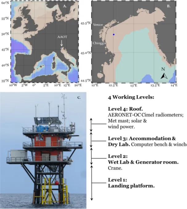
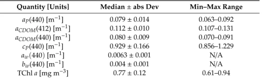
The field intercomparison was conducted at the Acqua Alta Oceanographic Tower (AAOT) which is located in the Gulf of Venice, Italy, in the northern Adriatic Sea at 45.31◦N, 12.51◦E during July 2018. The AAOT is a purpose-built steel tower with a platform containing an instrument house to facilitate the measurement of ocean properties under stable conditions such as clear skies, low wind speed and calm sea state (Figure1). The platform has a long history of optical measurements to support and validate both NASA and European Space Agency (ESA) ocean colour missions [32–34].
An autonomous optical measurement system was developed at the tower in 2002, the data from which are widely used and accessed by the ocean colour community for satellite validation via the AERONET-OC network [35,36]. The ocean circulation in the north western Adriatic region where the tower is located, is mainly influenced by the coastal southward flow of the North Adriatic current and a North Adriatic (cyclonic) gyre in autumn [37,38]. The site is also influenced by discharge from northern Adriatic rivers: Piave, Livenza and Tagliamento [36]. The water type at the tower can vary depending on wind and swell conditions from clear open sea (for 60% of the time [35]) to turbid coastal.
The atmospheric aerosol type is mostly continental and determined by atmospheric input from the Po valley, although occasionally this changes to maritime type aerosols [34].
Remote Sens.2020,12, 1587 6 of 48
Remote Sens. 2020, 12, x FOR PEER REVIEW 7 of 50
Figure 1. (A) Map showing the location of the Acqua Alta Oceanographic Tower (AAOT) in Europe and (B) in the Northern Adriatic Sea; (C) schematic of the AAOT. For the intercomparison, the radiance sensors were located on the deployment platform on level 3, on a 6 m pole that raised them above the solar panels on level 4. A telescopic (Fireco) mast for the irradiance sensors was located in the eastern corner of level 4.
Measurements were made at 20 min intervals, from 08:00 to 13:00 UTC, over a discrete measurement period of 5 min (called “cast”), with all instruments having a synchronized start time so that the data collected were directly comparable. In-water C-OPS measurements were also coordinated to these times, though with a temporal delay that is inherent in the practicalities of the deployment. The PANTHYR above-water system is automated to measure every 20 min and was not synchronised to the other (manually-triggered) above-water measurements. In-water TriOS measurements were made immediately after the above-water casts, taking around six minutes for the downcast measurements. From all casts, the median, mean and standard deviation at each OLCI wavelength were calculated.
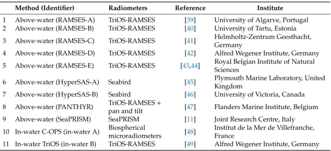
Table 1. Field intercomparison measurement systems, sensors and institutes. All sensors are hyperspectral except the bio-spherical which is multispectral.
Figure 1.(A) Map showing the location of the Acqua Alta Oceanographic Tower (AAOT) in Europe and (B) in the Northern Adriatic Sea; (C) schematic of the AAOT. For the intercomparison, the radiance sensors were located on the deployment platform on level 3, on a 6 m pole that raised them above the solar panels on level 4. A telescopic (Fireco) mast for the irradiance sensors was located in the eastern corner of level 4.
2.6. Participants and Data Submission
In total, 10 institutes participated in the intercomparison enabling the comparison of 11 measurement systems comprising 31 radiometers (Table 1). To rule out any differences arising from absolute radiometric calibration, all of the sensors used during the campaign were calibrated at the University of Tartu (UT), under the same conditions, within ~1 month of the campaign. The sensors were then shipped directly to Venice prior to setting up the campaign on 9 and 10 July 2018. Each participant was asked to submit their data ‘blind’, so that the overall results were not seen by participants prior to submission. ProcessedLsky,Lt,EdandRrsdata with application of OLCI’s spectral response function to obtain wavelengths corresponding to the OLCI channels (400, 412, 443, 490, 510, 560, 620,
665, 674, 681 nm) were submitted along with a UTC timestamp, the make, model, serial number of the instrument and integration time setting used during the acquisition.
Table 1. Field intercomparison measurement systems, sensors and institutes. All sensors are hyperspectral except the bio-spherical which is multispectral.
Method (Identifier) Radiometers Reference Institute 1 Above-water (RAMSES-A) TriOS-RAMSES [39] University of Algarve, Portugal 2 Above-water (RAMSES-B) TriOS-RAMSES [40] University of Tartu, Estonia 3 Above-water (RAMSES-C) TriOS-RAMSES [41] Helmholtz-Zentrum Geesthacht,
Germany
4 Above-water (RAMSES-D) TriOS-RAMSES [42] Alfred Wegener Institute, Germany 5 Above-water (RAMSES-E) TriOS-RAMSES [43,44] Royal Belgian Institute of Natural
Sciences
6 Above-water (HyperSAS-A) Seabird [45] Plymouth Marine Laboratory, United Kingdom
7 Above-water (HyperSAS-B) Seabird [46] University of Victoria, Canada 8 Above-water (PANTHYR) TriOS-RAMSES+
pan and tilt [47] Flanders Marine Institute, Belgium 9 Above-water (SeaPRISM) SeaPRISM [11] Joint Research Centre, Italy 10 In-water C-OPS (in-water A) Biospherical
microradiometers [48] Institut de la Mer de Villefranche, France
11 In-water TriOS (in-water B) TriOS-RAMSES [49] Alfred Wegener Institute, Germany
2.7. Radiometer Set-Up and Experimental Design
All above-water radiometers except the PANTHYR system were located on the same purpose-built frames (Figure2). The radiance sensors were located on the western corner of the AAOT and irradiance sensors and PANTHYR system were located at the eastern corner. For the radiance sensors, the frame was constructed to position the sensors side by side and at the same height (Figure2A). The frame was fabricated from aluminium at a height of 12.3 m from the sea surface. AllLskyandLtsensors had the same identical viewing zenith angles ofθ=40◦andθ0=140◦, respectively. A sundial was located mid-way down the mast of the frame with a vertical bar to turn it to the correct∆φ(Figure2B,C).
The deployment frame was adjusted for each measurement sequence so that∆φ=135◦or∆φ=90◦, which are typically used to reduce sun glint [18]. The radiance mast was positioned at the same level as the SeaPRISM system (Figure2B,C). The base of the mast was attached to a foldable knuckle joint so that the frame could be lowered, allowing for daily cleaning and servicing of the sensors.
For irradiance measurements, a telescopic (Fireco) mast was used to minimize interference from the tower super-structure and other overhead equipment which was installed at a height of 18.9 m above the sea surface (Figure1C, Figure2E,F).
Measurements were made at 20 min intervals, from 08:00 to 13:00 UTC, over a discrete measurement period of 5 min (called “cast”), with all instruments having a synchronized start time so that the data collected were directly comparable. In-water C-OPS measurements were also coordinated to these times, though with a temporal delay that is inherent in the practicalities of the deployment.
The PANTHYR above-water system is automated to measure every 20 min and was not synchronised to the other (manually-triggered) above-water measurements. In-water TriOS measurements were made immediately after the above-water casts, taking around six minutes for the downcast measurements.
From all casts, the median, mean and standard deviation at each OLCI wavelength were calculated.
Remote Sens.2020,12, 1587 8 of 48
Remote Sens. 2020, 12, x FOR PEER REVIEW 9 of 50
based on the generic Method 1 described in the Ocean Optics Protocols [50]. For the deployment and processing of data, all institutes followed published satellite validation protocols [5].
Figure 2. Photographs of the radiance sensors showing (A) the mounting for and radiometers, (B) location of sensors next to the AERONET-OC SeaPRISM, (C) location of the sensors on level 3 of the AAOT, (D) location of the irradiance sensors on the mounting block, (E) telescopic mast with irradiance sensors at the eastern corner of the AAOT, (F) proximity of the telescopic mast with irradiance sensors and the PANTHYR system just above the railings below.
2.8.2. TriOS Data Processing
For RAMSES sensors, data were acquired every 10 s for the duration of each 5 min cast (except RAMSES-C and -D which used burst mode) using TriOS’ proprietary MSDA XE software (except RAMSES-B who used their own code) and calibrated using the coefficients determined before the campaign by UT. Dark values were removed by the software’s “dynamic offset” function, which makes use of blocked photodiode array channels inside the radiometer to determine a background response signal in the absence of any measurable light. Using MSDA XE, the data output interval is 2.5 nm.
For RAMSES-A, the number of data records collected for each cast and radiometric sensor was 30. A bi-directional phase function f/Q correction [28] for wavelengths within 412 nm and 665 nm was also applied to account for the viewing and illumination geometry. For this the ℜ-tables from Gordon [26] were applied where the probability distribution of surface slope follows that of Ebuchi and Kizu [51].
For RAMSES-B, data were collected using bespoke Python software. The irradiance sensor had GPS time and location and tilt and heading devices located next to the sensor was a fish eye camera (see images from this in Figures A2 and A3). No corrections were applied but spectra with missing or saturated values were removed from the database.
RAMSES-C measurements were conducted in “burst mode” over the common 5 min casts which typically gave between 100 and 140 spectra. All spectra were used for averaging and determination of standard deviation; no flagging was applied (visual quality control confirmed expected natural variability for clear sky conditions). Both radiance spectra, and , were interpolated to the wavelengths of . The factor of Mobley [18] with roughness-considerations of Hieronymi [41] was used. The observed wave height was used to estimate the actual sea surface roughness [41]. If the observed significant wave height, Hs, was smaller than 0.5 m, “wind speed”
Figure 2.Photographs of the radiance sensors showing (A) the mounting forLskyandLtradiometers, (B) location of sensors next to the AERONET-OC SeaPRISM, (C) location of the sensors on level 3 of the AAOT, (D) location of the irradiance sensors on the mounting block, (E) telescopic mast with irradiance sensors at the eastern corner of the AAOT, (F) proximity of the telescopic mast with irradiance sensors and the PANTHYR system just above the railings below.
2.8. Above-Water Measurement Methods
All above-water systems measureEd,LtandLskywhich were interpolated to a spectral resolution of 1 nm. For each cast, the spectral response function for OLCI was applied to obtain the data at OLCI bands and the median, standard deviation and mean were calculated.Rrswas then computed using Equation (3). The HyperSAS and most RAMSES instrument systems used theρ0factor from [18] and the specific values for 90◦and 135◦azimuth viewing angle with respect to the sun plane or a variation on this theme (RAMSES-C), except for RAMSES-E (Table2).
2.8.1. TriOS-RAMSES
For above-water measurements RAMSES-A, -B, -C, -D and -E, three TriOS radiometers (TriOS Mess- und Datentechnik GmbH, Germany) were deployed by each institute; two RAMSES ARC-VIS hyperspectral radiance sensors for measuringLskyandLtrespectively, and one RAMSES ACC-VIS irradiance sensor for measuringEd. Measurements were made over the spectral range of 350–950 nm, with a resolution of approximately 10 nm, sampling approximately every 3.3 nm, with a spectral accuracy of 0.3 nm. The nominal full angle field-of-view (FOV) of the radiance sensors is 7◦. The sensors are based on the Carl Zeiss Monolithic Miniature Spectrometer (MMS 1) incorporating a 256-channel silicon photodiode array. Integration time varies from 4 ms to 8 s and is automatically adjusted based on measured light intensity to prevent saturation of the sensors. The data stream from all three instruments is integrated by an IPS-104 power supply and interface unit and logged on a PC via a RS232 connection. A two-axis tilt sensor is incorporated inside the downwelling irradiance sensor in some models. The basic measurement method used was developed by [43] based on the generic Method 1 described in the Ocean Optics Protocols [50]. For the deployment and processing of data, all institutes followed published satellite validation protocols [5].
2.8.2. TriOS Data Processing
For RAMSES sensors, data were acquired every 10 s for the duration of each 5 min cast (except RAMSES-C and -D which used burst mode) using TriOS’ proprietary MSDA XE software (except RAMSES-B who used their own code) and calibrated using the coefficients determined before the campaign by UT. Dark values were removed by the software’s “dynamic offset” function, which makes use of blocked photodiode array channels inside the radiometer to determine a background response signal in the absence of any measurable light. Using MSDA XE, the data output interval is 2.5 nm.
For RAMSES-A, the number of data records collected for each cast and radiometric sensor was 30.
A bi-directional phase function f/Q correction [28] for wavelengths within 412 nm and 665 nm was also applied to account for the viewing and illumination geometry. For this the<-tables from Gordon [26]
were applied where the probability distribution of surface slope follows that of Ebuchi and Kizu [51].
Table 2. Differences between laboratories in the processing of data fromEd,Lt, LskytoRrs. Year (Ed, Lsky,Lt) is the year of manufacture ofEd,Lsky,Lt/Lu/Eusensors; N are the number of replicates used for processing each cast; QC flag are quality control flags used; FOV is the radiance field of view;ρ0is the Fresnel reflectance factor used to process the data. For in-water-B, the number (N) reported forLtis actually N ofLu(z).
Sensor Type Year (Ed,Lsky,Lt) NEd NLsky NLt QC Flag FOV ρ0
RAMSES-A 2015, 2015, 2015 3–30 3–30 3–30 Visual QC 7◦ [18]
RAMSES-B 2004, 2006, 2010 3–30 3–30 3–30 Visual QC 7◦ [18]
RAMSES-C 2006, 2006, 2006 117–140 116–140 102–140 5 min scans 7◦ [18,41] * RAMSES-D 2007, 2006 **, 2011 123–141 4–90 4–54 Lt<1.5%;Lsky<
0.5% of min. 7◦ [18]
RAMSES-E 2008, 2001, 2001 1st 5 QC 1st 5 QC 1st 5 QC 1st 5 scans *** 7◦ [43,44]
HyperSAS-A 2006, 2006, 2006 280–345 284–398 93–198 5 min scans 6◦ [18,45]†
HyperSAS-B 2004, 2004, 2004 ~130 ~86 ~86 lower 20% 6◦ [18,46]
PANTHYR 2016, 2016# 2*3 2*3 11 See [45] 7◦ [18,47]
In-water A 2010, N/A, 2010 3–4 N/A 3–4 Visual QC N/A [18]
In-water B 2007, N/A, 2010 150–200 N/A ‡ ~86 7◦ [52]
* Using Mobley [18] and wave height correction of Hieronymi [41]; ** RAMSES-C Lsky sensor was used by lab RAMSES-D; *** The first five scans are taken as long as: (1) Inclination from the vertical does not exceed 5◦; (2)Ed,Lsky
orLtat 550 nm does not differ by more than 25% from either neighbouring scan; (3) the spectra are not incomplete or discontinuous;#One sensor used for bothLskyandLt;†Mean of 750–800 nm also removed;‡ForLu, average from 2 m–8 m was extrapolated to the surface (using 30–40 measurements). N/A means not applicable or measured.
For RAMSES-B, data were collected using bespoke Python software. The irradiance sensor had GPS time and location and tilt and heading devices located next to the sensor was a fish eye camera (see images from this in FiguresA2andA3). No corrections were applied but spectra with missing or saturated values were removed from the database.
RAMSES-C measurements were conducted in “burst mode” over the common 5 min casts which typically gave between 100 and 140 spectra. All spectra were used for averaging and determination of standard deviation; no flagging was applied (visual quality control confirmed expected natural variability for clear sky conditions). Both radiance spectra, Lsky andLt, were interpolated to the wavelengths ofEd. Theρfactor of Mobley [18] with roughness-considerations of Hieronymi [41] was used. The observed wave height was used to estimate the actual sea surface roughness [41]. If the observed significant wave height, Hs, was smaller than 0.5 m, “wind speed” was reduced by 30%
and the rounded values were used to selectρfrom Mobley’s look-up-tables (LUT) [18]. The usage of Mobley’sρ follows the rationale and comparisons of Zibordi [52] for this setup and conditions.
According to the institute’s protocol however, different sea surface reflectance factors are used to estimate uncertainties in the determination ofRrs. These reflectance factors are taken from the LUT of [18,41,44,53] depending on sun- and sensor-viewing geometry and wind speed, with one additional factor calculated fromLt/Lskyat 750 nm under the assumption that at this wavelength, water-leaving radiance is negligible for this site.
Remote Sens.2020,12, 1587 10 of 48
RAMSES-D followed protocol [54]. LtandEdwere recorded continuously throughout the day and the data for the casts were extracted for the five-minute measurement period. TwoEdsensors were used; an 81EA sensor (referred to as Sensor 1) and an 81E7 sensor (referred to as Sensor 2) for both the above water (RAMSES-D) and in-water (in-water B) measurements. NoLskysensor was available, so theLskydata from RAMSES-C were used. For each five-minute cast, theEddata were matched and extrapolated to the same time resolution ofLtandLskydata. Following the NASA and International Ocean Colour Coordinating Group (IOCCG) protocols [55,56],LtandLskymeasurements were corrected for variations inEdusing the medianEd. In order to minimize fluctuations within one cast, onlyLtandLsky, which were equal or less than 1.5% and 0.5% of the minimum ofLtandLskywith respect to the medianEd, were considered (Table2). After convoluting the finalLt,LskyandEdspectra to the original TriOS sensor resolution, the OLCI spectral response function were applied.
For RAMSES-E, full details of the data processing are described in [44] and associated appendices.
In brief, once the data were exported from the TriOS software, in-house Python scripts were used to implement several quality checks (QC), where a spectral scan was discarded if it met any of the following criteria: (a) inclination of the irradiance sensor exceeds 5◦from the vertical, (b)Ed,Lskyor Ltat 550 nm differ by more than 25% from either neighboring scan, (c)Lsky/Ed>0.05 sr−1at 750 nm (indicating clouds either in front of the sun or in the sky-viewing direction), or (d) the scan spectra is incomplete or discontinuous (occasional instrument malfunction). Once all scans for a given cast were processed through QC, only the first five scans (relative to the start time of the station) that had complete spectra for all three ofEd,LskyandLtwere used for further processing. From these data, “uncorrected” water-leaving radiance reflectance,R0w(θ,θ0,∆φ,λ), was calculated for each wavelength and for each of the five scans using Equations (1) and (3) above (with the distinction that R0w(θ,θ0,∆φ,λ)is equal toRrs(θ,θ0,∆φ,λ)multiplied by a factor ofπ). A simple quadratic function of wind speed forρwas used as approximation of the LUT of [18]. Minimization of perturbations due to wave effects was achieved through the turbid water near-infrared (NIR) similarity correction (Equation (8) in [43]). This was applied toR0w(θ,θ0,∆φ,λ)by determining the departure from the NIR similarity spectrum with:
ε= α1,2
·R0w(λ2)−R0w(λ1)
α1,2−1 , (7)
where wavelengthsλ1andλ2are chosen in the NIR, and the constantα1,2is set according to Equation (7) from [43] and Table 2of [44]. For this exercise, λ1 and λ2 were set to 780 nm and 870 nm respectively, generating a value ofα1,2=1.912. It is noted that this approach is similar to that proposed by [57], although relying on different wavelengths and values of sea surface reflectance. The NIR similarity-corrected water-leaving reflectance,Rw(λ), is then calculated as:
Rw(λ) =R0w(λ)−ε. (8)
A final pass of QC checks is performed on this NIR-correctedRw(λ)data, resulting in the entire station being discarded if the coefficient of variation (CV, standard deviation divided by the mean) of the five scans is>10% at 780 nm.
2.8.3. Seabird-HyperSAS
The measurement system consists of three hyperspectral Seabird (Washington, DC, USA; formerly SATLANTIC) spectro-radiometers, two measuring radiance and one measuring downwelling irradiance.
The sensors measure over the wavelength range 350–900 nm with a spectral sampling of approximately 3.3 nm and a spectral width of about 10 nm. Integration time can vary from 4 ms to 8 s and was automatically adjusted to the measured light intensity. The data stream from all three instruments is integrated by an interface unit and logged on a PC via a RS232 connection. The radiance sensors have a FOV of 6◦. Both HyperSAS-A and -B were first dark corrected in the same way; each instrument is equipped with a shutter that closes periodically to record dark values. TheEd,LtandLskydata were
first dark corrected by interpolating the dark value data in time, to match the light measurements for each sensor. Then dark values were subtracted from the light measurements at each wavelength.
TheEd,Lt andLskydata for both instrument systems were then interpolated to a common set of wavelengths (every 2 nm from 352–796 nm).
2.8.4. Seabird HyperSAS Data Processing
For HyperSAS-A, data processing follows “Method 1” of [53]. In brief, data were first extracted from the raw instrument files and the pre-campaign calibration coefficients were applied. Given that the optical conditions at the AAOT can often be considered Case 1 waters, besides the standard processing described for the other above-water sensors (no NIR correction), HyperSAS-A also implemented a processing method specific for open-ocean conditions (NIR correction). For NIR correction,Rrs(750) was subtracted from eachRrsspectrum. The effect of NIR and no NIR correction were compared.
For HyperSAS-B, data were processed using the lowest 20% values to minimize contamination by sky and sun glint.
2.8.5. The Pan-and-Tilt Hyperspectral Radiometer System (PANTHYR)
The PANTHYR is a new system designed for autonomous hyperspectral water reflectance measurements and described in detail in [47]. The instrument consists of two TriOS-RAMSES hyperspectral radiometers, mounted on a FLIR PTU-D48E pan-and-tilt pointing system, controlled by a single-board-computer and associated custom-designed electronics which provide power, pointing instructions, and data archiving and transmission. The TriOS radiometer specifications are the same as those outlined in Section2.8.1 above. The instrument is capable of full pan (±174◦) and tilt (+90◦/−30◦) movement. The radiance sensor is fixed at an angle of 40◦to the irradiance sensor, giving a zenith angle range for the irradiance sensor of 180◦(downwelling irradiance measurement) to 60◦ (parked) and a zenith angle range for the radiance sensor of 140◦(sky radiance measurement) through 40◦ (water radiance measurement) to 20◦ (parked). The PANTHYR system performs automated measurements every 20 min from sunrise until sunset. Each cycle consists of measurements with a 90◦, 135◦, 225◦, and/or 270◦relative azimuth to the sun. In general, and depending on the installation location, platform geometry, time of day (sun location), and associated platform shading of the water target, only one or two (or sometimes zero) of these azimuth angles are appropriate for measurement of water reflectance; other azimuth angles will be contaminated by platform shading or even direct obstruction of the water target as defined from the instrument FOV. A selection of acceptable azimuth angles is made a priori, based on expert judgement. For each measurement cycle, the system performs a sub-cycle for each of the configured relative azimuth angles. Based on the AERONET-OC protocol [8,22], but with repetition of theEdandLskyreplicates, each azimuthal measurement sub-cycle consists of 2×3 replicate scans each ofEdandLsky, and 11 replicate scans ofLt, where “scan” refers to acquisition of a single instantaneous spectrum. Firstly, the irradiance sensor is pointed upward, with the radiance sensor offset by 40◦, and three replicates of Ed followed by three replicates ofLskyare measured.
The radiance sensor is then moved to a 40◦downward viewing angle to make 11 replicateLtscans.
The irradiance and radiance sensors are then repositioned to make three more replicate scans of both LskyandEd. The PANTHYR system was deployed on the east side of the top deck of the platform (Figure2E), as opposed to the west side where the other above-water systems including AERONET-OC were located (Figure2B). The irradiance sensor collector was 2 m above the top deck floor and, hence, about 14 m above sea level as opposed to being located on the telescopic mast with the other irradiance sensors in the exercise and hence at 18.9 m above sea level.
2.8.6. PANTHYR Data Processing
LskyandLtscans with>25% difference between neighbouring scans at 550 nm were removed as well as any scans with incomplete spectra. Edscans were removed using the same criteria after normalizingEd by cos(θ0), whereθ0 is the sun zenith angle. The data are further processed if a
Remote Sens.2020,12, 1587 12 of 48
sufficient number of scans passes the quality control criteria: forLtthis is 9 of the possible 11 scans, and forEd andLskythis is 5 of the possible 6 scans. The remainingEdandLsky measurements are then grouped and mean-averaged. For eachLt scan,Lw (Equation (1)) is computed by removing sky-glint radiance using the look-up table (LUT) given in [18]. Wind speed was retrieved from ancillary data files in this intercomparison, but can alternatively be set to a user-defined default value if wind speed data are unavailable. The data in the LUT are linearly interpolated to the current observation geometry and wind speed. TheLwscans are then converted into “uncorrected” water-leaving radiance reflectanceR0w(θ,θ0,∆φ,λ)scans and NIR similarity spectrum correction is applied to remove any white error from inadequate sky-glint correction, following the “RAMSES-E” TriOS Data Processing sub-section in Section2.8.1 above. The final quality control to retain or reject the NIR corrected spectra,Rw(θ,θ0,∆φ,λ), is performed according to Ruddick et al. [44]. Measurements were rejected
whenLsky/Ed>0.05 sr−1at 750 nm (indicating clouds either in front of the sun or in the sky-viewing
direction), or when the coefficient of variation (CV, standard deviation divided by the mean) of the Rw(θ,θ0,∆φ,λ)scans was>10% at 780 nm.
2.8.7. SeaPRISM AERONET-OC
The SeaWiFS Photometer Revision for Incident Surface Measurements (SeaPRISM) is a modified CE-318 sun-photometer (CIMEL, Paris, France) that has the capability to perform autonomous above-water measurements. Measurements are made with a FOV of 1.2◦every 30 min in order to determineLwat a number of narrow spectral bands with centre-wavelengths of 412, 441, 488, 530, 551, 667 nm [32,35,36]. These measurements are: (1) the direct sun irradianceEs(Θ0,Φ0,λ)acquired to determine the aerosol optical thicknessτa(λ) used for the theoretical computation ofEd(0+,λ), and (2) a sequence of 11 sea-radiance measurements for determiningLt(θ,∆φ,λ)and of three sky radiance measurements for determiningLsky(θ,∆φ,λ). These sequences are serially repeated for eachλwith
∆φ=90◦,θ=40◦andθ0=140◦. The larger number of sea measurements, when compared to sky measurements, are required because of the higher environmental variability (mostly produced by wave perturbations) affecting the sea measurements during clear skies. Quality flags are applied at the different processing levels to remove poor data. Quality flags include checking for cloud contamination, high variance of multiple sea- and sky-radiance measurements, elevated differences between pre- and post- deployment calibrations of the SeaPRISM system, and spectral inconsistency of the normalized water-leaving radianceLwn[35]. The data are made available through the AERONET-OC web site (https://aeronet.gsfc.nasa.gov/new_web/ocean_color.html) version 3 to processing levels 1.5 and 2.
At the time of the field campaign, only level 1.5, real time cloud screened data were available, which were therefore used to compare against the other measurement systems. The difference between version 3 level 1.5 and 2 is in the application of post-deployment calibration and further QC checks.
On 13 July 2018, three coincident measurements were available; on 14 July four were available and on 17 July two were available. Of these, four were available at 21 min past the hour, when measurements from the above-water system were taken from 20–25 min past the hour. Five measurements were available at 49 min past the hour, when measurements from the above-water system were made between 40–45 min past the hour. The SeaPRiSM bands are centered at 412, 441, 488, 530, 551 and 667 nm. FromRrsabove-water hyperspectral data, using a spectrally flat window of 10 nm with±5 nm centered at the SeaPRISM bands, the average, median and standard deviation were computed and converted toLwnusing the BRDF function described in Section2.2(except for PANTHYR).
2.9. In-Water Methods
2.9.1. Compact Optical Profiling System (C-OPS)
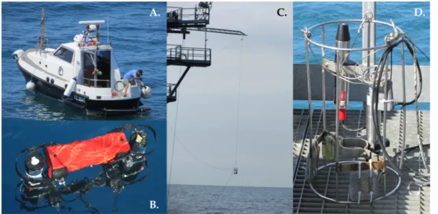
C-OPS (Biospherical Instruments Inc., USA) was designed specifically to operate in shallow coastal waters and from a wide range of deployment platforms [58,59]. The light sensors are mounted into a frame using a kite-shaped back plane with a hydrobaric chamber mounted along the top of the
profiler with a set of floats immediately below it (Figure3A,B). This allows the sensor to be vertically buoyant in the water column whilst ensuring that both light sensors are kept level (Figure3B). For this intercomparison exercise, the instrument was deployed at approximately 30 m distance from the stern of Research Vessel (RV)Litus(Figure3A) near coincident with the above-water measurements made on the AAOT. The surface reference sensor was mounted on a custom support on the foredeck of the RV Litus, and verticality was determined with a level when the ship was in port. For each cast, at least three consecutive profiles of upwelling nadir irradiance,Eu(t,z,λ), were acquired between surface and approximately 13 m depth, at the same time as the measurement of surface downwelling irradiance, Ed(t, 0+,λ). Both radiometers collected data at 20 Hz and included a pitch and roll sensor. A dark correction and a tare of depth were performed at least twice a day (at the beginning of the morning and afternoon casts). A second degree local polynomial fit function was used to interpolate and extrapolate Eu(t,z,λ)andEd(t, 0+,λ)in order to derive the upwelling irradiance just beneath the surface,Eu, and the surface irradiance at the beginning of the castEd(t0, 0+,λ), respectively. Data with an absolute tilt>10◦forEu(t,z,λ)and>20◦forEd(t, 0+,λ)were filtered out from the analysis. The fitted upwelling irradiance profile was corrected with a factor, ft(t), to account for possible variations in the surface irradiance:
ft(t) = Ed(t, 0+,λ)
Ed(t0, 0+λ). (9)
TheEuis corrected for radiometer self-shading following [48], where the absorption coefficient is estimated following [48] and initialized with the in situ total chlorophyll-a (TChla). TChlaused in the calculations was derived fromKd(443)[60] because the HPLC data were only analysed after the date of submission of the radiometry data. No correction was applied for the shading from the profiler, however theEusensor was deployed in a way that minimize this effect (i.e., with theEusensor side of the profiler oriented toward the sun). The water-leaving radiance,LW(λ), was calculated from the upwelling irradiance just below the sea surface as:
Lw(λ) =Eu(t0, 0−,λ)· 1 Q(θ0,TChla)·
(1−ρ0)
n2 , (10)
whereθ0 is the solar zenith angle (att0),ρ0 is the water–air interface Fresnel reflection coefficient (depending onθ0and sea roughness) andnis the refractive index of seawater for a flat surface and the Q(θ,TChla)factor is log-linearly interpolated from LUTs as provided in [28]. Theρ0is 0.043 and the refractive index of seawater,n, is 1.34. Aρ0of 0.02 is generally applied for a flat sea and uniform sky radiance andθ0<30◦and increases to 0.03 forθ0at 40◦. The values also increase with sea roughness.
Aρ0value of 0.043 is reported for a wind speed of 15 m s−1(θ0=30◦). The choice of 0.043 was made when the operational data processing was set to take into account average conditions at the deployment site for sea roughness andθ0 and was not modified as the difference in latitude with the AAOT is relatively low. Assuming 2% instead of 4.3% would have a limited impact on the comparison forRrs. Finally the remote-sensing reflectance was calculated using (Equation (3)) and shifted to OLCI central bands, when not coincident, following [31]. Specifically, C-OPS bands (λ1/2,COPS) at 395, 555/565, 625, 665/683 and 683 nm were shifted to 400, 560, 620, 674 and 681 nm, i.e., one wavelength is used when the wavelength difference is≤5 nm, two wavelengths are used when difference is>5 nm or two measurements with≤5 nm difference are available. Similarly, theEd(t0, 0+λ)was shifted to OLCI bands following:
Ed
t0, 0+,λOLCI
= Ed(t, 0+,λ1,COPS) Edth(t0, 0+,λ1,COPS)·Edth
t0, 0+,λOLCI
; ∆λ1≤5nm (11)
Remote Sens.2020,12, 1587 14 of 48
or
Ed(t0, 0+,λOLCI) =
(λOLCI−λ1,COPS) Ed(t,0+,λ1,COPS)
Edth(t0,0+,λ1,COPS)·Edth(t0,0
+λOLCI)+(λ2,COPS−λOLCI) Ed(t,0+,λ2,COPS)
Edth(t0,0+,λ2,COPS)·Edth(t0,0
+λOLCI)
λ2−λ1 ; ∆λ >5nm
or∆λ1and∆λ2≤5nm
(12)
where theEdth(t0, 0+,)denotes the theoretical surface irradiance for a clear sky and standard atmosphere computed from [26,61] using a spectrally flat window of 10 nm with±5 nm centered on the C-OPS and OLCI bands. The same correction scheme was applied for the comparison with the Sea-PRISM AERONET-OC with band shift from 443, 490, 532, 555, and 665 nm to 441, 488, 530, 551, and 667 nm.
Remote Sens. 2020, 12, x FOR PEER REVIEW 14 of 50
or
( , 0 , ) =
, , , ,
, , , ∙ ( , ) , , , ,
, , , ∙ ( , )
; 5
or ≤ 5
(12)
where the ( , 0 ,) denotes the theoretical surface irradiance for a clear sky and standard atmosphere computed from [26,61] using a spectrally flat window of 10 nm with ±5 nm centered on the C-OPS and OLCI bands. The same correction scheme was applied for the comparison with the Sea-PRISM AERONET-OC with band shift from 443, 490, 532, 555, and 665 nm to 441, 488, 530, 551, and 667 nm.
Figure 3. In-water sensors (A) C-OPS being deployed from RV Litus, (B) positioning of C-OPS in- water, (C) in-water TriOS deployment from an extendable boom on the AAOT, (D) TriOS in-water irradiance sensor in metal deployment frame.
2.9.2. In-Water TriOS-RAMSES
Hyperspectral TriOS-RAMSES radiometers, (Figure 3D) measured profiles of upwelling radiance, , and downwelling irradiance, , following the methods outlined in [49,54]. All measurements were collected with sensor-specific automatically adjusted integration times (between 4 ms and 8 s). The radiance and irradiance sensors were deployed from an extendable boom to 12 m off the south western corner of the AAOT (Figure 3C). The height of the boom was 12 m above sea surface, and is designed to reduce shadow and scatter from the tower. The sensor was equipped with an inclination and a pressure sensor. For this study, we only used the depth and inclination information from this sensor. During the intercomparison, the in-water inclination in either dimension was <6° [54]. For all casts, the instruments were first lowered to just below the surface, at approximately 0.5 m, for 2 min to adapt them to the ambient water temperature. The frame was then lowered to approximately 14 m, with stops every 1 m for a period of 30 s each, to obtain representative average values at each depth. Data were directly extracted from the calibrated instrument files applying the pre-campaign calibration coefficients and factory supplied immersion factors from the last factory calibration (2016) to obtain in water calibrations. Following the NASA and IOCCG protocols [55,56], ( , , ) data were corrected for incident sunlight (e.g., changing due to varying cloud cover) using simultaneously obtained downwelling irradiance ( ) measured above the water surface with another hyperspectral RAMSES irradiance sensor (either RAMSES-D Sensor 1 or Sensor 2) which was located on the telescopic mast on level 4 of the AAOT (Figure 2D–F). As surface waves strongly affect measurements in the upper few meters,
Figure 3.In-water sensors (A) C-OPS being deployed fromRV Litus, (B) positioning of C-OPS in-water, (C) in-water TriOS deployment from an extendable boom on the AAOT, (D) TriOS in-water irradiance sensor in metal deployment frame.
2.9.2. In-Water TriOS-RAMSES
Hyperspectral TriOS-RAMSES radiometers, (Figure3D) measured profiles of upwelling radiance, Lu, and downwelling irradiance,Ed, following the methods outlined in [49,54]. All measurements were collected with sensor-specific automatically adjusted integration times (between 4 ms and 8 s).
The radiance and irradiance sensors were deployed from an extendable boom to 12 m offthe south western corner of the AAOT (Figure3C). The height of the boom was 12 m above sea surface, and is designed to reduce shadow and scatter from the tower. TheEdsensor was equipped with an inclination and a pressure sensor. For this study, we only used the depth and inclination information from this sensor. During the intercomparison, the in-water inclination in either dimension was<6◦[54]. For all casts, the instruments were first lowered to just below the surface, at approximately 0.5 m, for 2 min to adapt them to the ambient water temperature. The frame was then lowered to approximately 14 m, with stops every 1 m for a period of 30 s each, to obtain representative average values at each depth. Data were directly extracted from the calibrated instrument files applying the pre-campaign calibration coefficients and factory supplied immersion factors from the last factory calibration (2016) to obtain in water calibrations. Following the NASA and IOCCG protocols [55,56],Lu(t,z,λ)data were corrected for incident sunlight (e.g., changing due to varying cloud cover) using simultaneously obtained downwelling irradianceEd+(λ)measured above the water surface with another hyperspectral RAMSES irradiance sensor (either RAMSES-DEdSensor 1 or Sensor 2) which was located on the telescopic mast on level 4 of the AAOT (Figure2D–F). As surface waves strongly affect measurements in