Marine isoprene production and consumption in the mixed layer of the surface ocean – a field study over two oceanic regions

(1)

https://doi.org/10.5194/bg-15-649-2018

Marine isoprene production and consumption in the mixed layer of the surface ocean – a field study over two oceanic regions

Dennis Booge¹, Cathleen Schlundt², Astrid Bracher^3,4, Sonja Endres¹, Birthe Zäncker¹, and Christa A. Marandino²

1GEOMAR Helmholtz Centre for Ocean Research, Kiel, Germany

2Marine Biological Laboratory, MBL, Woods Hole, MA, USA

3Alfred Wegener Institute – Helmholtz Centre for Polar and Marine Research, Bremerhaven, Germany

4Institute of Environmental Physics, University of Bremen, Germany Correspondence:Dennis Booge (dbooge@geomar.de)

Received: 21 June 2017 – Discussion started: 29 June 2017

Revised: 24 November 2017 – Accepted: 9 December 2017 – Published: 1 February 2018

Abstract.Parameterizations of surface ocean isoprene concentrations are numerous, despite the lack of source/sink pro- cess understanding. Here we present isoprene and related field measurements in the mixed layer from the Indian Ocean and the eastern Pacific Ocean to investigate the production and consumption rates in two contrasting regions, namely oligotrophic open ocean and the coastal upwelling region.

Our data show that the ability of different phytoplankton functional types (PFTs) to produce isoprene seems to be mainly influenced by light, ocean temperature, and salinity.

Our field measurements also demonstrate that nutrient availability seems to have a direct influence on the isoprene production. With the help of pigment data, we calculate in-field isoprene production rates for different PFTs under varying biogeochemical and physical conditions. Using these new calculated production rates, we demonstrate that an additional significant and variable loss, besides a known chemical loss and a loss due to air–sea gas exchange, is needed to explain the measured isoprene concentration. We hypothesize that this loss, with a lifetime for isoprene between 10 and 100 days depending on the ocean region, is potentially due to degradation or consumption by bacteria.

1 Introduction

Isoprene (2-methyl-1,3-butadiene, C₅H₈), a biogenic volatile organic compound (VOC), accounts for half of the total global biogenic VOCs in the atmosphere (Guenther et al., 2012). Globally, 400–600 Tg C yr⁻¹is emitted from terres-

trial vegetation (Guenther et al., 2006; Arneth et al., 2008).

Emitted isoprene influences the oxidative capacity of the atmosphere and acts as a source for secondary organic aerosols (SOAs) (Carlton et al., 2009). It reacts with hydroxyl radicals (OH), as well as ozone and nitrate radicals (Atkinson and Arey, 2003; Lelieveld et al., 2008), forming low-volatility species, such as methacrolein or methyl vinyl ketone, which are then further photooxidized to SOAs via more semi- volatile intermediate products (Carlton et al., 2009). Model studies suggest that isoprene accounts for 27 % (Hoyle et al., 2007), 48 % (Henze and Seinfeld, 2006), or up to 79 % (Heald et al., 2008) of the total SOA production globally.

Whereas the terrestrial isoprene emissions are well known to act as a source for SOAs, the oceanic source strength is hotly debated (Carlton et al., 2009). Marine-derived isoprene emissions only account for a few percent of the total emissions and are suggested, based on model studies, to be generally lower than 1 Tg C yr⁻¹ (Palmer and Shaw, 2005;

Arnold et al., 2009; Gantt et al., 2009; Booge et al., 2016).

Some model studies suggest that these low emissions are not enough to control the formation of SOAs over the ocean (Spracklen et al., 2008; Arnold et al., 2009; Gantt et al., 2009;

Anttila et al., 2010; Myriokefalitakis et al., 2010). However, due to its short atmospheric lifetime of minutes to a few hours, terrestrial isoprene does not reach the atmosphere over remote regions of the oceans. In these regions, oceanic emissions of isoprene could play an important role in SOA formation on regional and seasonal scales, especially in association with increased emissions during phytoplankton blooms (Hu et al., 2013). In addition, the isoprene SOA yield could be

(2)

up to 29 % under acid-catalyzed particle phase reactions during low-NO_xconditions, which occur over the open oceans (Surratt et al., 2010). This SOA yield is significantly higher than a SOA burden of 2 % during neutral aerosol experiments calculated by Henze and Seinfeld (2006).

Marine isoprene is produced by phytoplankton in the euphotic zone of the oceans, but only a few studies have directly measured the concentration of isoprene to date, and the exact mechanism of isoprene production is not known. The concentrations generally range between<1 and 200 pmol L⁻¹ (Bonsang et al., 1992; Milne et al., 1995; Broadgate et al., 1997; Baker et al., 2000; Matsunaga et al., 2002; Broadgate et al., 2004; Kurihara et al., 2010; Zindler et al., 2014; Ooki et al., 2015; Hackenberg et al., 2017). Depending on region and season, concentrations of isoprene in surface waters can reach up to 395 and 541 pmol L⁻¹during phytoplankton blooms in the highly productive Southern Ocean and Arc- tic waters, respectively (Kameyama et al., 2014; Tran et al., 2013).

Studies have shown that the depth profile of isoprene mainly follows the chlorophyll a (chl a) profile, suggesting phytoplankton as an important source (Bonsang et al., 1992; Milne et al., 1995; Tran et al., 2013; Hackenberg et al., 2017); furthermore, Broadgate et al. (1997) and Kuri- hara et al. (2010) show a direct correlation between isoprene and chl a concentrations in surface waters and between 5 and 100 m depth, respectively. However, this link is not consistent enough on global scales to predict marine isoprene concentrations using chl a (Table 1). Laboratory studies with different monocultures illustrate that the isoprene production rate varies widely depending on the phytoplankton functional type (PFT) (Booge et al., 2016, and references therein). In addition, environmental parameters, such as temperature and light, have been shown to influence isoprene production (Shaw et al., 2003; Exton et al., 2013; Meskhidze et al., 2015). In general, the production rates increase with increasing light levels and higher temperature, similar to the terrestrial vegetation (Guenther et al., 1991). However, this trend cannot easily be generalized to all species, because each species-specific growth requirement is linked differently to the environmental conditions. For example, Srikanta Dani et al. (2017) showed that two diatom species, Chaetoceros calcitransandPhaeodactylum tricor- nutum,have their maximum isoprene production rate at light levels of 600 and 200 µmol m⁻²s⁻¹, respectively, which decreases at even higher light levels. Furthermore, Meskhidze et al. (2015) measured the isoprene production rates of different diatoms at different temperature and light levels on two consecutive days. Their results showed a less variable but higher emission on day two, suggesting that phytoplankton must acclimate physiologically to the environment. This should also hold true for dynamic regions of the ocean and has to be taken into account when using field data to model isoprene production.

The main loss of isoprene in seawater is air–sea gas exchange, with a minor physical loss due to advective mixing and chemical loss by reaction with OH and singlet oxygen (Palmer and Shaw, 2005). The existence of biological losses still remains an open question, as almost no studies were conducted concerning this issue. Shaw et al. (2003) assumed the biological loss by bacterial degradation to be very small. However, Acuña Alvarez et al. (2009) showed that isoprene consumption in culture experiments from marine and coastal environments did not exhibit first-order dependency on isoprene concentration. They observed faster isoprene consumption with lower initial isoprene concentration.

This study significantly increases the small dataset of marine isoprene measurements in the world oceans with new observations of the distribution of isoprene in the surface mixed layer of the oligotrophic subtropical Indian Ocean and in the nutrient-rich upwelling area of the eastern Pa- cific Ocean along the Peruvian coast. These two contrasting and, in terms of isoprene measurements, highly undersam- pled ocean basins are interesting regions in which to compare the diversity of isoprene-producing species. With the help of concurrently measured physical (temperature, salinity, radiation), chemical (nutrients, oxygen), and biological (pigments, bacteria) parameters, we aim to improve the understanding of isoprene production and consumption processes in the surface ocean under different environmental conditions.

2 Methods 2.1 Sampling sites

Measurements of oceanic isoprene were performed during three separate cruises, the SPACES (Science Partnerships for the Assessment of Complex Earth System Processes) and OASIS (Organic very short lived substances and their Air–

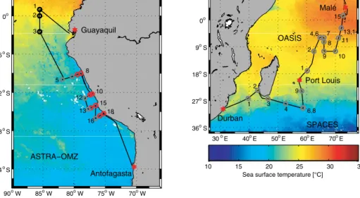
Sea exchange from the Indian Ocean to the Stratosphere) cruises in the Indian Ocean and the ASTRA-OMZ (Air–Sea interaction of TRAce elements in Oxygen Minimum Zones) cruise in the eastern Pacific Ocean. The SPACES and OA- SIS cruises took place in July/August 2014 on board the R/V Sonne I from Durban, South Africa, via Port Louis, Mauritius, to Malé, Maldives; the ASTRA-OMZ cruise took place in October 2015 on board the R/V Sonne II from Guayaquil, Ecuador, to Antofagasta, Chile (Fig. 1).

2.2 Isoprene measurements

During all cruises, up to seven samples (50 mL) from 5 to 150 m depth for each depth profile were taken bubble-free from a 24 L Niskin bottle rosette equipped with a CTD (conductivity–temperature–depth; described in Stramma et al., 2016). Ten milliliters of helium was put into each transparent glass vial (Chromatographie Handel Müller, Fridolfing, Germany), replacing the same amount

(3)

Table 1.Factors of different regression equations ([isoprene]=u×[chla]+v×SST+intercept) from different studies compared to factors from this study. Bold, italic, and regular R²value: correlation significant, not significant, and significance not known, respectively (significant:p <0.05). [chla] in µg L⁻¹, SST in^◦C, [isoprene] in pmol L⁻¹.

Reference Cruise (region) SST bins u v Intercept R²

Hackenberg et al. (2017) AMT 22 (Atlantic O.) <20^◦C 37.9 – 17.5 0.37(n=39)

AMT 23 (Atlantic O.) 15.1 – 18.4 0.55(n=11)

ACCACIA 2 (Arctic) 34.1 – 11.1 0.61(n=34)

AMT 22 (Atlantic O.) ≥20^◦C 300 – −3.35 0.60(n=93)

AMT 23 (Atlantic O.) 103 – 5.58 0.82(n=22)

Ooki et al. (2015) Southern Ocean, Indian Ocean, Northwest Pacific Ocean, Bering Sea, western Arctic Ocean

3.3–17^◦C 14.3 2.27 2.83 0.64

17–27^◦C 20.9 −1.92 63.1 0.77

>27^◦C 319 8.55 −244 0.75

Kurihara et al. (2012) Sagami Bay No bin 10.7 – 5.9 0.49(n=8)

Kurihara et al. (2010) Western North Pacific No bin 18.8 – 6.1 0.79(n=60)

Broadgate et al. (1997) North Sea No bin 6.4 – 1.2 0.62

This study Whole study No bin 2.45 – 22.1 0.07(n=138)

SPACES (Indian Ocean) 20.2 – 8.01 0.30(n=37)

OASIS (Indian Ocean) 42.6 – 12.6 0.10(n=59)

ASTRA-OMZ (eastern South Pacific O.)

1.26 – 26.5 0.07(n=42)

<20^◦C 3.92 – 11.5 0.59(n=46)

≥20^◦C 25.6 – 16.6 0.14(n=92) 3.3–17^◦C 1.30 10.0 −144 0.84(n=10) 17–27^◦C 10.4 0.76 −3.70 0.41(n=97)

>27^◦C 40.4 −0.58 39.7 0.17(n=31)

of sea water and providing a headspace for the upcoming analysis. The water samples were, if necessary, stored in the fridge and analyzed on board, within 1 h of collection, using a purge-and-trap system attached to a gas chromatograph–

mass spectrometer (GC-MS; Agilent 7890A/Agilent 5975C;

inert XL MSD with triple-axis detector) (Fig. 2). Isoprene was purged for 15 min from the water sample with helium (70 mL min⁻¹) containing 500 µL of gaseous deuter- ated isoprene (d5-isoprene) as an internal standard to account for possible sensitivity drift (Fig. 2: purge unit, load position). The gas stream was dried using potassium carbonate (SPACES and OASIS) or a Nafion^r membrane dryer (Perma Pure; ASTRA-OMZ). CO₂- and hydrocarbon-free dry, pressurized air with a flow of 180 mL min⁻¹was used as counter flow in the Nafion^rmembrane dryer (Fig. 2: water removal). Before being injected into the GC (Fig. 2: trap unit, inject position), isoprene was preconcentrated in a Sulfinert^r stainless-steel trap (1/16 in. OD) cooled with liquid nitrogen (Fig. 2: trap unit, load position). The mass spectrometer was operated in single-ion mode, quantifying isoprene and d5-

isoprene usingm/z ratios of 67 and 68, and 72 and 73, respectively. In order to perform daily calibrations for quantifi- cation, gravimetrically prepared liquid isoprene standards in ethylene glycol were diluted in Milli-Q water and measured in the same way as the samples. The precision for isoprene measurements was±8 %.

2.3 Nutrient measurements

Micronutrient samples were taken on every cruise from the CTD bottles (covering all sampled depths). The samples from SPACES were stored in the fridge at−20^◦C and measured during OASIS. Samples from OASIS and ASTRA- OMZ were directly measured on board with a QuAAtro auto- analyzer (Seal Analytical). Nitrate was measured as nitrite following reduction on a cadmium coil. The precision of nitrate measurements was calculated to be±0.13 µmol L⁻¹.

(4)

90ôW 85ôW 80ôW 75ôW 70ôW 24ôS

18ôS 12ôS 6ôS 0ô

Guayaquil

Antofagasta ASTRA−OMZ

30ôE 40ôE 50ôE 60ôE 70ôE 36ôS

27ôS 18ôS 9ôS 0ô

Durban

Port Louis Malé

SPACES OASIS

Sea surface temperature [°C]

10 15 20 25 30 35

1 2 3

5 8

10 12

13 15 16

18

1 2

3

4 6,8 9

1 2

4,6 7 8 9 10

11 13,14 15

Figure 1.Cruise tracks (black) of ASTRA-OMZ (October 2015, eastern Pacific Ocean) and of SPACES and OASIS (July/August 2014, Indian Ocean) plotted on top of monthly mean sea surface temperature detected by the Moderate Resolution Imaging Spectroradiometer (MODIS) instrument on board the Aqua satellite. Circles indicate CTD stations (grey: SPACES and OASIS as well as open-ocean stations during ASTRA-OMZ; black: equatorial stations during ASTRA-OMZ; red: coastal stations during ASTRA-OMZ). Numbers indicate stations where a CTD depth profile was performed. Stations 6 and 8 (SPACES) as well as stations 4 and 6, and 13 and 14 (OASIS) have almost the same geographical coordinates. If a station number is omitted (SPACES: stations 5 and 7; OASIS: stations 3, 5, and 12; ASTRA-OMZ:

stations 4 and 9), no CTD cast was performed.

Figure 2.Schematic overview of the analytical purge-and-trap system, divided into three parts: purge unit(a), water removal(b), and trap unit(c). He: helium; MFC: mass flow controller; K₂CO₃: potassium carbonate; GC-MS: gas chromatograph–mass spectrometer.

2.4 Bacteria measurements

For bacterial cell counts, 4 mL samples were preserved with 200 µL glutaraldehyde (1 % v/v final concentration) and stored at −20^◦C for up to 3 months until measurement.

A stock solution of SYBR Green I (Invitrogen) was prepared by mixing 5 µL of the dye with 245 µL dimethyl sulfoxide (Sigma Aldrich). Ten microliters of the dye stock solution and 10 µL of Fluoresbrite YG microspheres beads (diameter 0.94 µm, Polysciences) were added to 400 µL of the thawed sample and incubated for 30 min in the dark. The samples were then analyzed at low flow rate using a flow cytome-

ter (FACSCalibur, Becton Dickinson) (Gasol and Del Gior- gio, 2000). Trucount beads (Becton Dickinson) were used for calibration and in combination with Fluoresbrite YG micro- sphere beads (0.5–1 µm, Polysciences) for absolute volume calculation. Calculations were done using the software pro- gram “CellQuest Pro”.

2.5 Phytoplankton functional types from marker pigment measurements

Different PFTs were derived from marker phytoplankton pigment concentrations and chlorophyll concentrations. To determine PFT chl a, 0.5 to 6 L of sea water was filtered

(5)

through Whatman GF/F filters at the same stations where isoprene was sampled. The soluble organic pigment concentrations were determined using high-pressure liquid chro- matography (HPLC) according to the method of Barlow et al. (1997), adjusted to our temperature-controlled instru- ments as detailed in Taylor et al. (2011). We determined the list of pigments shown in Table 2 of Taylor et al. (2011) and applied the method by Aiken et al. (2009) for qual- ity control of the pigment data. PFT chl a was calculated using the diagnostic pigment analysis developed by Vidussi et al. (2001) and adapted in Uitz et al. (2006).

This method uses specific phytoplankton pigments which are (mostly) common only in one specific PFT. These pigments are called marker or diagnostic pigments (DPs), and the method relates for each measurement point the weighted sum of the concentration of seven DPs, representa- tive of each PFT, to the concentration of monovinyl chlorophyll a concentration; in doing so, PFT group-specific coefficients are derived which enable the PFT chl a concentration to be derived. The latter is a ubiquitous pigment in all PFTs except Prochlorococcus, which contains divinyl chlorophyll a instead. In general, chl a is a valid proxy for the overall phytoplankton biomass. In the DP analysis, concentrations of fucoxanthin, peridinin, 19’hexanoyloxy- fucoxanthin, 19’butanoyloxy-fucoxanthin, alloxanthin, and chlorophyllbare used as DPs indicative of diatoms, dinoflagellates, haptophytes, chrysophytes, cryptophytes, cyanobacteria (excludingProchlorococcus), and chlorophytes, respectively. With the DP analysis then finally the chlaconcentration of these PFTs were derived. The chla concentration of Prochlorococcuswas directly derived from the concentration of divinyl chlorophylla.

2.6 Photosynthetically available radiation within the water column measurements

Since no underwater light data were available for all cruises, we used global radiation data from the ship’s meteorological station together with the light attenuation coefficients (determined from the chlaconcentration profiles) to calculate the photosynthetically available radiation (PAR) within the water column during a day. In detail we processed these data the following way.

We fitted the hourly resolved global radiation data with a sine function to account for the light variation during the day and converted into PAR just above surface, PAR(0⁺) in µmol m⁻²s⁻¹during the course of a day, by multiplying these daily global radiation values with a factor of 2 (Jaco- vides et al., 2004) (Fig. S1a).

The subsurface PAR (PAR(0⁻)) was calculated using the refractive index of water (n=1.34) and 0.98 for transmis- sion assuming incident light angles<49^◦:

PAR(0⁻)=E_dPAR(0⁺)×1.34²/0.98. (1)

In order to derive the diffuse attenuation coefficient for PAR (K_dPAR), we calculated the euphotic depth (Z_eu) from the chlaprofile for all stations using the approximation by Morel and Berthon (1989), which was further refined by Morel and Maritorena (2001). In detail the following was done: from the chlaprofiles at each station the total chlaintegrated for Z_eu(C_tot) was determined. A given profile was progressively integrated with respect to increasing depth (z). The successive integrated chla values were introduced in Eqs. (2) and (3) accordingly, thus providing successive Z_eu values that were progressively decreasing. Once the lastZ_eu value, as obtained, became lower than the actual depthzused when integrating the profile, these Ctot andZeu values from the last integration were taken. Profiles which did not reachZeu

were excluded.

Z_eu=912.5×C_tot^−0.839; if 10 m< Z_eu<102 m (2) Z_eu=426.3×C_tot^−0.547; ifZ_eu>102 m (3) K_dPAR of each station was then calculated fromZ_eu as follows:

KdPAR= 4.6 Zeu

. (4)

The plane photosynthetically available irradiance at each depth (z) in the water column, PAR(z), was then calculated applying Beer–Lambert’s law (Fig. S1b):

PAR(z)=PARsurface×e^−K^d^z. (5)

An example of two PAR fitted depth profiles for the time of the two specific stations is shown in the Supplement (Fig. S2), which have been compared to directly measured downwelling photosynthetically available radiation (E_dPAR) profiles. The comparison shows that the fitted PAR profiles obtained from the ship’s global radiation data and chlorophyll profiles were reliable.

E_dPAR profiles were only measured during ASTRA day- time stations with a hyperspectral radiometer (RAMSES, TriOS GmbH, Germany) covering a wavelength range of 320 to 950 nm with an optical resolution of 3.3 nm and a spectral accuracy of 0.3 nm (for more details on the measurements see Taylor et al., 2011). The downwelling irradianceEd(z, λ) RAMSES data were interpolated to 1 nm resolution, and then theEd(z) given in watts per square meter (W m⁻²) at each nanometer wavelength step between 400 and 700 nm was converted to micromolar quanta per square meter per second (µmol quanta m⁻²s⁻¹) to micromolar quanta per square by following the principle that one photon contains the energy E_p=(h×c)/λ (with the Planck’s constant h=6.6266× 10⁻³⁴Js and the speed of light c=299 792 458 m s⁻¹). Fi- nally, the E_d(z, λ) were integrated from 400 to 700 nm to receive the downwelling photosynthetically available plane irradiance (E_dPAR(z)).

(6)

Table 2.Emission factor (EF) of each PFT determined by applying a log-squared relationship between light intensity and isoprene production rates resulting from published phytoplankton culture experiments.

PFT Emission factor References of literature values used for fitting^a

Diatoms 0.0064 Shaw et al. (2003), Bonsang et al. (2010), Exton et al. (2013), Meskhidze et al. (2015) Chlorophytes 0.0168 Shaw et al. (2003), Bonsang et al. (2010), Exton et al. (2013)

Dinoflagellates 0.0176 Exton et al. (2013)

Haptophytes 0.0099 Shaw et al. (2003), Bonsang et al. (2010), Exton et al. (2013) Cyanobacteria 0.0097 Shaw et al. (2003), Bonsang et al. (2010), Exton et al. (2013) Cryptophytes 0.0120 Exton et al. (2013)

Prochlorococcus 0.0053 Shaw et al. (2003)

aExact species within a PFT tested for calculation production rates can be found in the references cited for each PFT.

2.7 Calculation of isoprene production

We calculated the isoprene production rate (P) in two different ways: a direct and an indirect calculation, which will be explained in the following paragraphs. For all calculations made, we came up with one production rate per station within the mixed layer. This was either due to the shallow mixed- layer depth (MLD) resulting in only one measurement within the mixed layer (coastal stations ASTRA-OMZ) or due to well-mixed isoprene concentrations showing almost no gradient within the mixed layer (data explained in Sect. 3.2).

2.7.1 Direct calculation of isoprene production rates Isoprene production rates of different PFTs were determined in laboratory phytoplankton culture experiments (see a collection of literature values: Table 2 in Booge et al., 2016) and were used here to calculate isoprene production from measured PFTs in the field. These literature studies showed that isoprene production rates are light dependent, with increasing production rates at higher light levels (Shaw et al., 2003;

Gantt et al., 2009; Bonsang et al., 2010; Meskhidze et al., 2015). To include the light dependency in our calculations, we followed the approach of Gantt et al. (2009) for each PFT by applying a log-squared fit between all single literature laboratory chl-a-normalized isoprene production rates Pchloro

(µmol isoprene (g chla)⁻¹h⁻¹) (references in Table 2) and their measured light intensityI (µmol m⁻²s⁻¹) during individual experiments to determine an emission factor (EF) for each PFT (Fig. S3):

Pchloro=EF×ln(I )². (6)

The resulting EF from this log-squared fit is unique for each PFT and is listed in Table 2: the higher the EF of a PFT, the higher its P_chloro value at a specific light intensity. It should be noted that we are not sure what species were actually present during the cruises. We realize, therefore, that this method of calculating EFs is limited. In order to calculate the isoprene production at each sampled depth (z) at each station, we used the scalar photosynthetically available

radiation in the water column, PAR(z) (see Sect. 2.6), as in- put forI, which was used with the respective calculated EF of each PFT using Eq. (6). The product was integrated over the course of the day, resulting in aPchlorovalue (µmol isoprene (g chla)⁻¹ day⁻¹) for each PFT and day depending on the depth in the water column (Fig. S4). The light- and depth-dependent individualP_chloro,_i values of each PFT at the sampled depthz were multiplied with the corresponding measured PFT chla concentration ([PFT]_i). The sum of all products gives the directly calculated isoprene production rate at each sampled depthz:

P_direct(z)=X

P_chloro_i× [PFT]_i

. (7)

Integrating over all measurements within the mixed layer and scaling with the MLD results in a “mean” direct isoprene production rate (Pdirect) for each station.

2.7.2 Indirect calculation of isoprene production rates The indirect calculation of the isoprene production rate is dependent on our measured isoprene concentrations (C_Wmeasured). We used the simple model concept of Palmer and Shaw (2005), assuming that the measured isoprene concentration is in steady state, meaning that the production (P) is balanced by all loss processes:

P−C_Wmeasured

Xk_CHEM,_iC_Xi+k_BIOL+ k_AS MLD

(8)

−L_MIX=0,

wherekCHEMis the chemical loss rate constant for all possible loss pathways (i) with the concentrations of the reac- tants (C_X=OH and O₂), kBIOL is the biological loss rate constant due to biological degradation, andL_MIXis the loss due to physical mixing. These constants are further described in Palmer and Shaw (2005).k_ASis the loss rate constant due to air–sea gas exchange scaled with the MLD. The MLD at each station was calculated from CTD profile measurements, applying the temperature threshold criterion (±0.2^◦C) of de Boyer Montégut et al. (2004).k_ASwas computed using the

(7)

Schmidt number (SC) of isoprene (Palmer and Shaw, 2005) and the quadratic wind-speed-based (U₁₀) parameterization of Wanninkhof (1992):

kAS=0.31U₁₀² S_C

660 −0.5

. (9)

As we assume steady-state isoprene concentration, we used the mean wind speed and the mean sea surface temperature (SST) of the last 24 h of shipboard observations before taking the isoprene sample to calculateU10 andSC, respectively.

We modified Eq. (8) to calculate the needed production rate (P_need) by multiplyingCWmeasured with the sum of k_CHEM(0.0527 day⁻¹) andk_ASscaled with the MLD:

P_need=C_Wmeasured

k_CHEM+ kAS

MLD

. (10)

We neglected the loss rates of isoprene due to biological degradation and physical mixing because they are low compared to k_CHEM and k_AS (Palmer and Shaw, 2005; Booge et al., 2016), meaning that the resultingP_need value can be seen as a minimum needed production rate.

3 Results and discussion 3.1 Cruise settings

The first part of the Indian Ocean cruise, SPACES, started in Durban and traveled eastwards, passing the Agulhas current and the southern tip of Madagascar (Toliara reef) with relatively warm water masses (mean: 23.4^◦C) and southerly winds. Southeast of Madagascar wind direction changed to easterly winds, and we encountered the Antarctic circumpo- lar current with significantly lower mean sea surface temperatures of 19.7^◦C before heading north to Mauritius. Mean wind speed during the cruise was 8.2±3.7 m s⁻¹, and mean salinity was 35.5±0.2. Global radiation over the course of the day was on average ∼360±70 W m⁻². As shown in Fig. 3, within the mixed layer, chlaconcentrations were very low (average value<0.3 µg L⁻¹) during the whole cruise, coinciding with generally low nutrient levels in the mixed layer (mean values for nitrate and phosphate were 0.14 and 0.15 µmol L⁻¹, respectively).

The second part of the Indian Ocean cruise, OASIS, cov- ered open-ocean regimes and upwelling regions, such as the equatorial overturning cell as described in Schott et al. (2009) and the shallow Mascarene Plateau (8–12^◦S, 59–62^◦E).

Constant southeasterly winds (mean: 10.3±4.2 m s⁻¹) were observed that were characteristic for the season of the south- west monsoon. During the cruise, sea surface temperature was constantly increasing with latitude from 24.4^◦C (Port Louis) to 29.7^◦C (southern tip of the Maldives)

with mean daily light levels of ∼457±64 W m⁻². Salin- ity ranged from 34.4 to 35.4. As for the SPACES cruise, the chla concentration in the western tropical Indian Ocean was low (0.2–0.5 µg L⁻¹ on average, Fig. 3). Nitrate levels (mean: 0.42 µmol L⁻¹) in the mixed layer were higher than during SPACES, but phosphate levels were not (mean:

0.17 µmol L⁻¹).

The ASTRA-OMZ cruise took place in the coastal, wind- driven Peruvian upwelling system (16^◦S–6^◦S). This area is a part of one of the four major eastern boundary upwelling systems (Chavez and Messié, 2009) and is highly influenced by the El Niño–Southern Oscillation. We observed constant southeasterly winds (8.2±2.5 m s⁻¹) traveling par- allel to the Peruvian coast. During neutral surface conditions or La Niña conditions, cold, nutrient-rich water is being upwelled at the shelf of Peru, resulting in high biological productivity. However, in early 2015 a strong El Niño developed, which brought warmer, low-salinity waters from the western Pacific to the coast of Peru, resulting in suppressed upwelling with lower biological activity due to the presence of nutrient- poor water masses. The cruise started with a section passing the Equator from north to south at 85.5^◦W east of the Gala- pagos Islands with mean sea surface temperatures of 25.0^◦C and low-salinity waters (mean for profiles: 34.2), as well as low chlaconcentrations (mean for profiles: 0.5 µg L⁻¹). Lev- els of incoming shortwave radiation were∼508±67 W m⁻². Afterwards, we performed four onshore–offshore transects at about 9, 12, 14, and 16^◦S off the coast of Peru (Fig. 1), where the incoming shortwave radiation was significantly decreased by clouds (∼300 W m⁻²). Upwelled waters, identi- fied by higher salinity (mean: 35.2) and lower sea surface temperatures (mean: 18.9^◦C), were found during the second part of the cruise. Chla values were highest directly at the coast (max: 13.1 µg L⁻¹), coinciding with lower sea surface temperatures (Fig. 3), showing that some upwelling was still present.

3.2 Isoprene distribution in the mixed layer

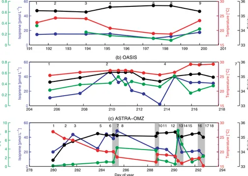
The isoprene concentrations during the SPACES cruise were generally very low, ranging from 6.1 to 27.1 pmol L⁻¹ in the mixed layer (mean for the average of a profile:

12.3 pmol L⁻¹) in the southern Indian Ocean, mainly due to very low biological productivity. During the OASIS cruise, the isoprene concentrations south of 10^◦S were comparable to the concentrations of the SPACES cruise. North of 10^◦S, the isoprene values in the mixed layer were significantly higher (mean: 35.9 pmol L⁻¹) (Fig. 3). These results are in good agreement with the sea surface isoprene concentrations of Ooki et al. (2015) in the same area east of 60^◦E, who measured concentrations lower than 20 pmol L⁻¹ south of 12^◦S and concentrations of∼40 pmol L⁻¹north of 12^◦S during a campaign between November 2009 and Jan- uary 2010. During ASTRA-OMZ the concentrations ranged from 12.7 to 53.2 pmol L⁻¹ with a mean isoprene concen-

(8)

0 20 40 60

Isoprene [pmol L]−1

33 34 35 36

Salinity

0 0.2 0.4 0.6 0.8

chl a [µg L]−1

191 192 193 194 195 196 197 198 199 200 15201

20 25 30

Temperature [°C]

1 2 3 4 6 8 9

(a) SPACES

0 20 40 60

33 34 35 36

Salinity

0 0.2 0.4 0.6 0.8

chl a [µg L]−1

204 206 208 210 212 214 216 21815

20 25 30

Temperature [°C]

1 2 4 6 7 8 9 10 11 13 14 15

(b) OASIS

0 20 40 60

33 34 35 36

Salinity

0 2 4 6 8 10

chl a [µg L]−1

278 280 282 284 286 288 290 292 29415

20 25 30

Temperature [°C]

1 2 3 5 6 7 8 10 11 12 13 14 15 16 17 18 (c) ASTRA−OMZ

Day of year

Figure 3.Mean salinity (black), isoprene concentration (blue), temperature (red), and chlaconcentration (green) in the MLD at each station during SPACES(a), OASIS(b), and ASTRA-OMZ(c). Grey rectangles highlight the eight coastal stations during ASTRA-OMZ. Numbers in each panel refer to the corresponding station number.

tration of 29.5 pmol L⁻¹ in the mixed layer. Although the chlaconcentrations at the coastal stations (3.8 µg L⁻¹) were significantly higher than open-ocean values (0.7 µg L⁻¹), the isoprene values did not show the same trend (Fig. 3).

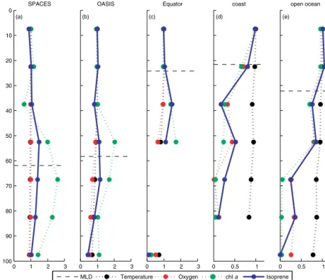
A mean normalized depth profile of each cruise for isoprene (blue), water temperature (black), oxygen (red), and chl a (green) is shown in Fig. 4. In order to compare the depth profiles of each cruise with respect to the different concentration regimes, we normalized the measured values by dividing the concentration of each depth of each station by the mean concentration in the mixed layer from the same station profile. A normalized value>1 means that the value at a certain depth is higher than the mean value in the mixed layer; a value<1 means less than in the mixed layer. As the sampled depths at each station were not the same on every cruise, we binned the data into seven equally spaced depth intervals (15 m) and averaged each data of an interval over each of the three cruises. The calculated mean mixed-layer depths of the SPACES and OASIS cruises, using the temperature threshold criterion (±0.2^◦C) of de Boyer Montégut et al. (2004), were about 60 m; the mean mixed-layer depth of the ASTRA-OMZ cruise was 30 m, excluding the four coastal stations, which had a MLD of only 20 m, resulting in only one bin interval in the MLD. Figure 4 shows that during all three cruises almost no gradient of isoprene in the mixed layer was detectable. In contrast to the isoprene concentration, the highest chla concentration was measured slightly above or below the MLD during SPACES/OASIS, whereas

during ASTRA-OMZ chla showed the same trend as isoprene. These results suggest a very fast mixing of isoprene after it is produced by phytoplankton and released to the water column above the MLD.

As isoprene is produced biologically by phytoplankton, many studies have attempted to find a correlation between chla and isoprene, finding very different results. Bonsang et al. (1992), Milne et al. (1995), and Zindler et al. (2014) did not find a significant correlation, whereas other studies could show a significant correlation and, therefore, attempted a linear regression to show a relationship between isoprene and chla, as well as SST (Broadgate et al., 1997; Kurihara et al., 2010, 2012; Ooki et al., 2015; Hackenberg et al., 2017).

Comparing the different factors of each regression equation (Table 1), it can be seen that, even if the correlations for most of the datasets are significant, there is no globally unique regression factor to adequately describe the relationship between chla (and SST) and isoprene. As shown in Table 1, during ASTRA-OMZ there was no significant correlation between chlaand isoprene, whereas during SPACES and OA- SIS the correlation was significant but with lowR² values (SPACES:R²=0.30; OASIS:R²=0.10) and different regression coefficients. Hackenberg et al. (2017) split their data from three different cruises into two SST bins with SST values higher and lower than 20^◦C, resulting in significant correlations withR²values from 0.37 to 0.82 depending on the cruise (Table 1). Ooki et al. (2015) described a multiple linear relationship between isoprene, chla, and SST when us-

(9)

0 0.5 1 (d)

ASTRA−OMZ coast

0 0.5 1

(e) ASTRA−OMZ

open ocean

0 1 2 3

0

10

20

30

40

50

60

70

80

90

100 (a)

SPACES

Depth [m]

0 1 2 3

(b) OASIS

0 1 2 3

(c) ASTRA−OMZ

Equator

MLD Temperature Oxygen chl a Isoprene

Figure 4.Mean normalized depth profiles of temperature (black), oxygen (red), chla(green), and isoprene (blue) during(a)SPACES,(b) OASIS, and(c, d,e)ASTRA-OMZ. The black dashed line represents the mean MLD for each cruise.

ing three different SST regimes (Table 1). Our correlations, using the approaches of Ooki et al. (2015) and Hackenberg et al. (2017), were significant, except for SST values higher than 27^◦C, but the regression coefficients were also significantly different to those found by Ooki et al. (2015) and Hackenberg et al. (2017). These varying equations demonstrate that bulk chlaconcentrations, or linear combinations of chl a concentration and SST, do not adequately predict the variability of isoprene in the global surface ocean, but they do point to these variables as among the main controls on isoprene concentration in the euphotic zone.

3.3 Modeling chl-a-normalized isoprene production rates

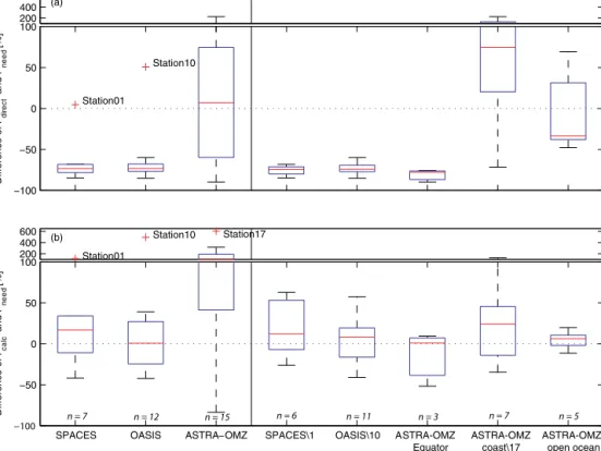
The directly calculated production rate (Pdirect) using Eq. (7) and the indirectly calculated production rate (Pneed) using Eq. (10) were compared and were found to be significantly different (Fig. 5a; difference in percent: (Pdirect− Pneed)/Pneed×100). The difference of more than−70 % be- tweenPdirect andPneed during SPACES and OASIS means that P_direct is too low to account for the measured isoprene concentrations, which is also true for the equatorial region of ASTRA-OMZ. In the open-ocean region of ASTRA-OMZ, the average difference betweenP_directandP_needis the lowest but still highly variable from station to station. However, in the coastal region of ASTRA-OMZ the directly calculated isoprene production rate greatly overestimates the needed

production by 75 % on average. There are three possible ex- planations for this difference: (1) the presence of a missing sink, which is not accounted for in the calculation ofPneed. Adding an additional loss term to Eq. (10) would increase the needed production to reach the measured isoprene concentration. This sink would only be valid for this specific coastal region but would increase the discrepancy between P_directandP_needfor all other performed cruises. Furthermore, this possible loss rate constant would have to be on average 0.22 day⁻¹and, therefore, higher than the main loss due to air–sea gas exchange in the coastal region (see Sect. 3.5 and Fig. 8). Thus, it is highly unlikely that this additional loss term is the only reason for the discrepancy betweenPdirect

andPneed. (2) Another possible explanation arises from the uncertainty of using a light-dependent log-squared fit. Mea- surements from different laboratory studies used different species within one group of PFTs. All species within one PFT group were combined to produce a light-dependent isoprene production rate (Fig. S3), although the isoprene production variability of different species within one PFT group is quite high. This will certainly influenceP_directbut cannot explain the 70 % difference betweenP_direct andP_need measured during SPACES and OASIS and during ASTRA-OMZ (Equator) (Fig. 5). (3) An incorrect literature-derived chl-a- normalized isoprene production rate (P_chloro) for one or more groups of PFTs is another possible explanation. For example, the highP_directvalues, compared to theP_needvalues, during ASTRA-OMZ coincided with high chla concentrations in

(10)

the coastal area. These coastal stations were, in contrast to all other measured stations, highly dominated by diatoms (up to 7.67 µg L⁻¹, Fig. S5). This might point to a possibly incorrect P_chlorovalue (too high) for diatoms (and other PFTs).

Therefore, we calculated new individual chl a normalized production rates of each PFT (P_chloronew) within the MLD. We used the concentrations of haptophytes, cyanobacteria, and Prochlorococcus for SPACES and OASIS and the concentrations of haptophytes, chlorophytes, and diatoms for ASTRA-OMZ, as these PFTs were the three most abundant PFTs of each cruise, accounting on average for≥80 % of total PFTs. We performed a multiple linear regression by fitting a linear equation between the Pneed values for each station and the corresponding PFT chl a concentrations (analogous to Eq. 7) to derive one new calculated Pchloronew value for each PFT and cruise, which is listed in Table 3. The lower and upper limit of the Pchloronewvalue was set to 0.5 and 50 µmol (g chla)⁻¹day⁻¹, respectively, when performing the multiple linear regression to avoid mathematically possible but biologically un- reasonable negative chl-a-normalized isoprene production rates. The upper limit was chosen in relation to the maximum published chl-a-normalized isoprene production rate ofPrasinococcus capsulatusby Exton et al. (2013) (32.16± 5.76 µmol (g chla)⁻¹day⁻¹). This rate was measured during common light levels of 300 µmol m⁻²s⁻¹. Applying a same log-squared relationship between light levels and the isoprene production rate as for the other PFTs would increase this value up to 50 µmol (g chl a)⁻¹ day⁻¹ at light levels of∼1000 µmol m⁻²s⁻¹. Our tests using the whole PFT com- munity for the multiple linear regression did not change our results and, in some cases, led to highly unlikely production rates for the less abundant PFTs.

With the help of the multiple-linear-regression-derived P_chloronewvalues, we calculated the new direct isoprene production rate (P_calc) in the same way asP_directin Eq. (7). We compared our calculatedP_calc values with theP_need values which are shown in Fig. 5b (difference in percent between P_calcandP_need). We found one outlier station for each cruise (SPACES: station 1; OASIS: station 10; ASTRA-OMZ: station 17) when using the newP_chloronewvalues for each PFT for each whole cruise (Fig. 5b, left part). We excluded these stations from every following calculation and redid the multiple linear regression. Furthermore, we split the ASTRA- OMZ into three different regions (Equator, coast, and open ocean), due to their contrasting biomass-to-isoprene concentration ratio, and calculated newPchloronewvalues for each of the three most abundant PFTs for SPACES, OASIS, and each part of ASTRA-OMZ.

Haptophytes were one of the three most abundant PFTs during all three cruises (Fig. S5), and their P_chloronew values range from 0.5 to 47.9 µmol (g chl a)⁻¹ day⁻¹ with a mean value of 17.9±18.3 µmol (g chl a)⁻¹day⁻¹for all cruises. The haptophyte production rates exhibited two interesting features. First, this range is highly variable depend-

ing on the oceanic region (tropical ocean (SPACES), subtropical ocean (OASIS)) and different ocean regimes (coast, open ocean). Second, the average value is different from the mean value of all laboratory-study-derived isoprene production rates of haptophytes (6.92±5.78 µmol (g chla)⁻¹day⁻¹, Table 3). During SPACES and OASIS the P_chloronew values of Prochlorococcus (both 0.5 µmol (g chl a)⁻¹ day⁻¹) are slightly lower but in good agreement with the mean literature value (1.5 µmol (g chl a)⁻¹ day⁻¹, Ta- ble 3), whereas the cyanobacteria values are higher (44.7 and 13.9 µmol (g chl a)⁻¹ day⁻¹) than the literature value (6.04 µmol (g chl a)⁻¹ day⁻¹, Table 3). Chloro- phytes and are known to be low isoprene producers, with mean Pchloro values of 1.47 µmol (g chl a)⁻¹ day⁻¹ and 2.51 µmol (g chl a)⁻¹ day⁻¹, respectively (Table 3). For diatoms, this is verified with our calculated rates during ASTRA-OMZ (all values≤ 0.6 µmol (g chl a)⁻¹ day⁻¹), whereas the rate for chlorophytes in the coastal regions (6.1 µmol (g chla)⁻¹ day⁻¹)is significantly higher than in the open ocean and equatorial region during ASTRA-OMZ (0.5 µmol (g chla)⁻¹ day⁻¹). Over all three cruises no significant correlations were found between the new multiple- linear-regression-derivedP_chloronewvalues of each PFT and any other parameter measured on the cruise. This may be caused by the high variability of the chla normalized production rates of different PFTs (Table 3). Another explanation could be the high variability of isoprene production of different species within one PFT group. For in- stance, in the PFT group of haptophytes, the isoprene production rates of two different strains of Emiliania huxleyi measured by Exton et al. (2013) were 11.28 ± 0.96 and 2.88±0.48 µmol (g chla)⁻¹ day⁻¹ for strain CCMP 1516 and CCMP 373, respectively. Laboratory culture experiments show that stress factors, like temperature and light, also influence the emission rate within one species (Shaw et al., 2003; Exton et al., 2013; Meskhidze et al., 2015). Srikanta Dani et al. (2017) showed that in a light regime of 100–

600 µmol m⁻²s⁻¹the isoprene emission rate was constantly increasing with higher light levels for the diatom Chaeto- ceros calcitrans, whereas the diatomPhaeodactylum tricor- nutum was highest at 200 µmol m⁻²s⁻¹ and decreased at higher light levels. Furthermore, health conditions (Shaw et al., 2003), as well as the growth stage of the phytoplankton species (Milne et al., 1995), can also influence the isoprene emission rate.

With the new Pcalc values, we slightly overestimate the needed productionPneedby up to 20 % on average (Fig. 5b, right part). For SPACES and OASIS, except for stations 1 and 10, using oneP_chloronewvalue for each PFT for the whole cruise is reasonable because the biogeochemistry in these regions did not differ much within one cruise. This was not true for ASTRA-OMZ, due to the biogeochemically contrasting open-ocean region and the coastal upwelling region. Using just oneP_chloronew value for each PFT for the whole cruise resulted in a highly overestimated and variableP_calc value

(11)

Figure 5.Percent differences between(a)P_directandP_need((P_direct−P_need)/P_need) and(b)P_calcandP_need((P_calc−P_need)/P_need) for the different cruises/cruise regions. Left of the vertical black line, data are divided into the three different cruises; right of the vertical black line, data are shown for the three cruises with outliers from the left part excluded. Additionally, ASTRA-OMZ was split into three regions (Equator, coast, open ocean). Number of stations (n) used for each set of data are shown in italics. The red line represents the median, the boxes show the first to third quartile, and the whiskers illustrate the highest and lowest values that are not outliers. The red plus signs represent outliers. The number indicated after\denotes a station that has been excluded from the analysis.

Table 3.Calculated chl-a-normalized isoprene production rates (P_chloronew, µmol (g chla)⁻¹day⁻¹) of the three most abundant PFTs during SPACES and OASIS (haptophytes, cyanobacteria,Prochlorococcus) and ASTRA-OMZ (haptophytes, chlorophytes, diatoms). Number indicated after\denotes a station that has been excluded from the analysis. For explanation of the omission, please refer to Sect. 3.3.

Cruise Haptophytes Cyanobacteria Prochlorococcus Chlorophytes Diatoms

SPACES\1 0.5 44.7 0.5 – –

OASIS\10 21.2 13.9 0.5 – –

ASTRA-OMZ Equator 47.9 – – 0.5 0.5

Coast\17 9.6 – – 6.1 0.6

Open ocean 10.3 – – 0.5 0.5

Collection of literature values in Booge et al. (2016) 6.92 6.04 1.5^a 1.47 2.51^a

aProduction rates from Arnold et al. (2009) were excluded from literature values listed in Booge et al. (2016).

(Fig. 5b, “ASTRA-OMZ”). Therefore splitting this cruise into three different parts (Equator, coast, open ocean), due to their different chla concentration and nutrient availability, resulted in less variableP_calcvalues. However, in the coastal region, the variability is still the highest, but with the newly derivedP_calcthe agreement withP_needis significantly better than withP_direct(compare Fig. 5a and b).

3.4 Drivers of isoprene production

As mentioned above, no significant correlations between each calculatedP_chloronewvalue and any other parameter during the three cruises were found.Prochlorococcuswas one of the three most abundant PFTs during SPACES and OA- SIS, but concentrations decrease to almost zero in the colder open-ocean and upwelling regions of ASTRA-OMZ (Fig. 1), which confirms the general knowledge thatProchlorococcus

(12)

300 400 500

Radiation [W m−2]

(a)

0 20 40 60

Pchloronew haptophytes [µmol(g chl a) day]−1−1

15 20 25 30

Ocean temp. [°C]

(b)

33.5 34 34.5 35 35.5

Salinity

(c)

SPACES OASIS ASTRA-OMZ

Equator

ASTRA-OMZ coast

ASTRA-OMZ open ocean 0

10 20

NO3− [µmol L−1] (d)

Figure 6.Mean values (±SD) for(a)calculatedP_chloronewhaptophytes (blue line) and global radiation (yellow bars),(b)ocean temperature, (c)salinity, and(d)nitrate during SPACES, OASIS, and ASTRA-OMZ (split into three different parts: Equator, coast, and open ocean).

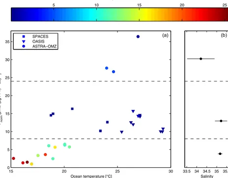
is absent at temperatures<15^◦C (Johnson et al., 2006). Our newly derived production rates confirm the actual laboratory- derived rates, demonstrating Prochlorococcus as a minor contributor to isoprene concentration. However, Prochloro- coccus is especially abundant at high ocean temperatures, where isoprene production rates from the other PFTs show evidence of decreasing. Cyanobacteria concentrations (ex- cludingProchlorococcus) were also related to temperature, but, in contrast toProchlorococcus, other cyanobacteria taxa can be abundant in colder waters during ASTRA-OMZ. The different derived isoprene production rates for SPACES and OASIS might be related to the different mean ocean temperature and light levels during these cruises. During SPACES, with lower ocean temperatures and lower light levels than OASIS, the production rate is higher. This relationship would confirm the findings of two independent laboratory studies of Bonsang et al. (2010) and Shaw et al. (2003). Bonsang et al. (2010) tested two species of cyanobacteria at 20^◦C and found higher isoprene production rates than a different species tested by Shaw et al. (2003) at 23^◦C and even stronger light intensities. However, Exton et al. (2013) measured the same rate as Shaw et al. (2003) at 26^◦C for one species, but a 5-times-higher production rate for another species at the same temperature. Because we do not know which species were present, we hypothesize that the production rate is not dependent on one environmental parameter and varies from species to species within the group of cyanobacteria.

Comparing the calculated isoprene production rates of the haptophytes with global radiation, ocean temperature, salinity, and nitrate results in some interesting qual-

itative trends (Fig. 6). Mean global radiation during SPACES (∼360 W m⁻²) was lower than during OASIS (∼457 W m⁻²). Highest mean values were measured during ASTRA-OMZ (at the Equator,∼508 W m⁻²). The same trend can be seen in theP_chloronewvalues of the haptophytes.

Within the open-ocean and coastal regimes of ASTRA- OMZ, the isoprene production rate was lower than around the Equator (mean global radiation decreased to∼310 W m⁻²).

A similar trend can be seen with the mean ocean temperature and the P_chloronew values of the haptophytes. These results are similar to several laboratory experiments with monocultures: higher light intensities and water temperatures enhance phytoplankton ability to produce isoprene (Shaw et al., 2003; Exton et al., 2013; Meskhidze et al., 2015).

However, Meskhidze et al. (2015) showed in laboratory experiments that isoprene production rates from two diatoms species were highest when incubated in water temperatures of 22 to 26^◦C. Higher temperatures caused a decrease in isoprene production rate. During OASIS, mean water temperatures were 27.3^◦C and went up to 29.2^◦C near the Mal- dives. Increasing ocean temperatures influence the growth rate of phytoplankton generally, as well as differently within one group of PFTs. For haptophytes, Huertas et al. (2011) show that two strains ofEmiliania huxleyiwere not tolerant to a temperature increase from 22 to 30^◦C, whereasIsochry- sis galbana could adapt to the increased temperature. In general, the optimal growth rate temperature decreases with higher latitude (Chen, 2015), but the link between growth rate of phytoplankton and isoprene production rate is still not known. Assuming this temperature dependence can be transferred from diatoms also to haptophytes, the high sea-

(13)

water temperatures during OASIS could explain why the calculated isoprene production rate is lower than in the ASTRA- OMZ equatorial regime. Additionally, as mentioned before, the temperature as well as the light dependence of isoprene production might vary between different species of haptophytes when comparing different ocean regimes. Another reason for the very high isoprene production rate of haptophytes in the equatorial regime during ASTRA-OMZ, apart from temperature and light intensity, could be stress-induced production caused by low-salinity waters, which was already shown for dimethylsulfoniopropionate, a precursor for the climate-relevant trace gas dimethyl sulfide (DMS), produced by phytoplankton (Shenoy et al., 2000). The salinity is con- siderably lower at the Equator during ASTRA-OMZ than for all other cruise regions, with values down to 33.4. We observed that the Pchloronew values decrease again in regions with more saline waters, where phytoplankton likely experi- ences less stress due to salinity, temperature, or light levels (Fig. 6).

In order to identify parameters that influence not only the chl-a-normalized isoprene production rate of haptophytes but the rate of all PFTs together, we calculated a normalized isoprene production rate (P_norm) independent from the absolute amount of each PFT. Hence, we divided eachP_calcvalue at every station by the amount of the three most abundant PFTs:

P_norm=

3

P

i=1

P_chloronew_i× [PFT]_i

3

P

i=1

[PFT]_i

= Pcalc 3

P

i=1

[PFT]_i

, (11)

whereiis three most abundant PFTs during each cruise.

The P_norm value helps us to obtain more insight about the influencing factors at each station, rather than only one mean data point for each cruise. We plotted the P_norm values of each station vs. the ocean temperature and color- coded them by nitrate concentration as a marker for the nutrient availability (Fig. 7). During SPACES (squares) and OA- SIS (triangles), the normalized production rate is on average 12.8±2.2 pmol(µg PFT)⁻¹day⁻¹and independent from the ocean temperature, while the nitrate concentration is very low (0.33±0.53 µmol L⁻¹). During ASTRA-OMZ (circles) in the coastal and open-ocean regions, the nitrate concentrations were significantly higher (16.4±5.5 µmol L⁻¹), but the Pnorm values were lower (<8 pmol(µg PFT)⁻¹ day⁻¹), correlating with lower ocean temperatures. In the equatorial region of ASTRA-OMZ, the production rates are significantly higher than during SPACES and OASIS, at up to 36.4 pmol(µg PFT)⁻¹ day⁻¹. On the right panel of Fig. 7, the mean salinity for each P_norm-dependent box (separated by the dashed lines) is shown. ASTRA-OMZ (Equator) and SPACES and OASIS do not differ in ocean temperature or in nitrate concentration. However, the normalized production is

significantly higher at the ASTRA-OMZ equatorial region, which may be caused by the low salinity there. In summary, (1) during ASTRA-OMZ (coast, open ocean)Pnormis com- paratively lower (<8 pmol(µg PFT)⁻¹ day⁻¹) under “biogeochemically active” conditions (high nitrate concentration) but increases with increasing ocean temperature; (2) under limited-nutrient conditions P_norm is significantly increased likely due to nutrient stress; and (3) if the phytoplankton are additionally stressed due to lower salinity,P_norm is furthermore increased. These results show that there is no main parameter driving the isoprene production rate, resulting in a more complex interaction of physical and biological parameters influencing the phytoplankton to produce isoprene.

3.5 Loss processes

The comparison betweenPcalc andPneed in Fig. 5b shows a mean overestimation of 10–20 %. This is likely due to a missing loss term in the calculation, which would balance out the needed and calculated isoprene production. Chemical loss (red dashed line) and loss due to air–sea gas exchange (black solid line) using the gas transfer parameterization of Wanninkhof (1992) were already included in the calculation (Eq. 10), and their loss rate constants are shown in Fig. 8. For comparison, we added thek_ASvalues using the parameterizations of Wanninkhof and McGillis (1999) (black dotted line) and Nightingale et al. (2000) (black dashed line). They have different wind speed dependencies of gas transfer, which could influence the computed isoprene loss at high wind speeds. The parameterization of Wanninkhof and McGillis (1999) is cubic and will increase the loss rate constant of isoprene due to air–sea gas exchange at high wind speeds compared to the other parameterizations (Fig. 8, OASIS).

Nightingale et al. (2000) is a combined linear and quadratic parameterization, which would decrease the isoprene loss due to air–sea gas exchange. However, during SPACES and ASTRA-OMZ the wind speed was between 8 and 10 m s⁻¹, where the parameterization of Wanninkhof (1992) is higher than both Wanninkhof and McGillis (1999) and Nightingale et al. (2000). Therefore the use of these alternative parameterizations would even lower the loss rate constant due to air–sea gas exchange, leading to the need for an additional loss rate in order to balance the isoprene production.

To calculate the additionally required consumption rate (kconsumption), we only used stations where a loss term was actually needed to balance the calculated and needed production (P_calc> Pneed). Those values were averaged within each cruise and are shown in Fig. 8. For comparison, we added the loss rate constants due to bacterial consumption from Palmer and Shaw (2005) (blue dashed line; 0.06 day⁻¹) and an updated value from Booge et al. (2016) (blue dotted line; 0.01 day⁻¹). Comparable to the chemical loss rate, the k_BIOLvalues were assumed to be constant (following the as- sumption of Palmer and Shaw, 2005), because no data about bacterial isoprene consumption in surface waters are avail-