Supplement of Biogeosciences, 15, 649–667, 2018 https://doi.org/10.5194/bg-15-649-2018-supplement
© Author(s) 2018. This work is distributed under the Creative Commons Attribution 4.0 License.
Supplement of
Marine isoprene production and consumption in the mixed layer of the surface ocean – a field study over two oceanic regions
Dennis Booge et al.
Correspondence to:Dennis Booge (dbooge@geomar.de)
The copyright of individual parts of the supplement might differ from the CC BY 4.0 License.
Supplement
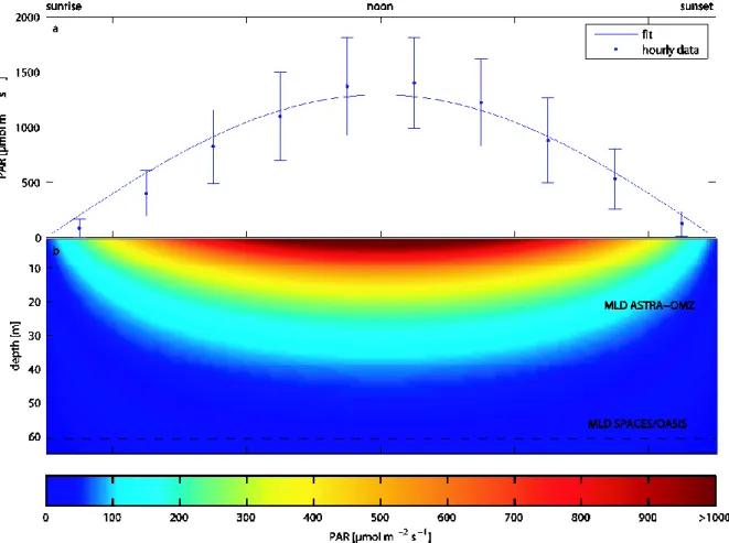
Figure S1: Example for above and in-water radiation. (a) Data points represent hourly radiation measurements (converted from W m-2 into photosynthetic active radiation (PAR, µmol m-2 s-1) as described in paragraph 2.6) from
5
the ship (mean values ± standard deviation from all cruises), blue line is the fitted data using a sine function. (b) Underwater mean calculated PAR over the course of a day depending on depth by applying the attenuation coefficient KdPAR and Beer-Lambert’s law. Dashed line represents mean mixed layer depth (MLD) for each cruise.
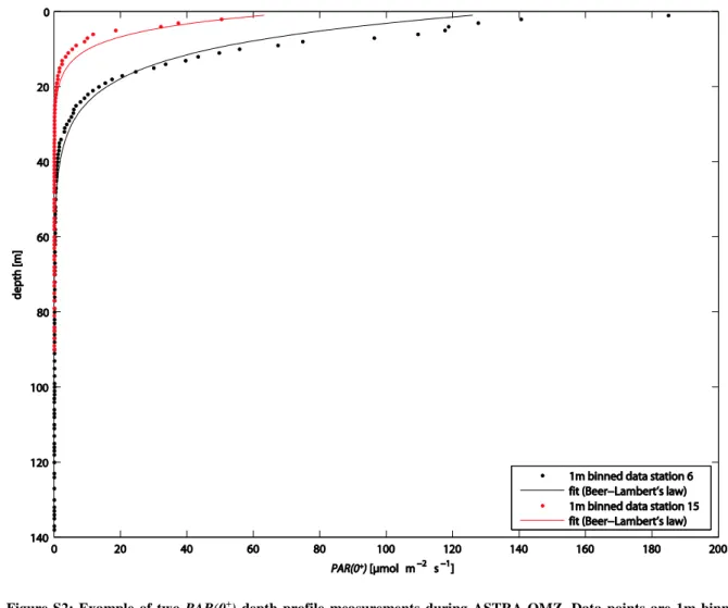
Figure S2: Example of two PAR(0+) depth profile measurements during ASTRA-OMZ. Data points are 1m binned
10
data of station 6 (black) and station 15 (red). The line is calculated from PAR(0+) by applying Beer-Lambert’s law using a mean attenuation coefficient KdPAR obtained from all EdPAR(0+) depth profile measurements during OASIS and ASTRA-OMZ.
15
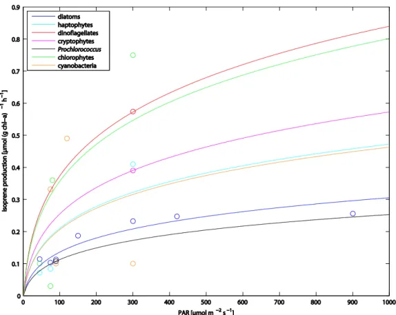
Figure S3: Single literature laboratory chl-a normalized isoprene production rates Pchloro (µmol isoprene (g chl-a)-1 h-1) (Table 2) as a log squared function of light intensity I (µmol m-2 s-1).
20
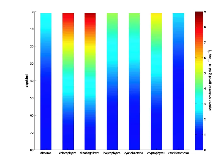
Figure S4: Example of calculated Pchloro values (µmol isoprene (g chl-a)-1 day-1) for each PFT at station 9 during SPACES depending on the depth in the water column.
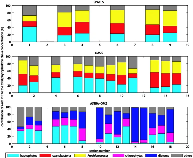
Figure S5: Contribution of each of the three most abundant PFTs to the total phytoplankton chl-a concentration at
25
each station during SPACES (upper panel), OASIS (middle panel), and ASTRA-OMZ (bottom panel).