The contribution of oceanic halocarbons to marine and free tropospheric air over the tropical West Pacific

(1)

www.atmos-chem-phys.net/16/7569/2016/

doi:10.5194/acp-16-7569-2016

The contribution of oceanic halocarbons to marine and free tropospheric air over the tropical West Pacific

Steffen Fuhlbrügge¹, Birgit Quack¹, Susann Tegtmeier¹, Elliot Atlas², Helmke Hepach¹, Qiang Shi³, Stefan Raimund⁴, and Kirstin Krüger⁵

1GEOMAR Helmholtz Centre for Ocean Research Kiel, Kiel, Germany

2Rosenstiel School for Marine and Atmospheric Sciences, Miami, Florida, USA

3Department of Oceanography, Dalhousie University, Halifax, Canada

4SubCtech GmbH, Roscoff, France

5Department of Geosciences, University of Oslo, Oslo, Norway Correspondence to:Kirstin Krüger (kirstin.krueger@geo.uio.no)

Received: 26 March 2015 – Published in Atmos. Chem. Phys. Discuss.: 2 July 2015 Revised: 30 April 2016 – Accepted: 12 May 2016 – Published: 21 June 2016

Abstract. Emissions of halogenated very-short-lived substances (VSLSs) from the oceans contribute to the atmospheric halogen budget and affect tropospheric and stratospheric ozone. Here, we investigate the contribution of natural oceanic VSLS emissions to the marine atmospheric boundary layer (MABL) and their transport into the free troposphere (FT) over the tropical West Pacific. The study con- centrates on bromoform, dibromomethane and methyl iodide measured on ship and aircraft during the SHIVA (Strato- spheric Ozone: Halogen Impacts in a Varying Atmosphere) campaign in the South China and Sulu seas in Novem- ber 2011. Elevated oceanic concentrations for bromoform, dibromomethane and methyl iodide of on average 19.9, 5.0 and 3.8 pmol L⁻¹, in particular close to Singapore and to the coast of Borneo, with high corresponding oceanic emissions of 1486, 405 and 433 pmol m⁻²h⁻¹respectively, characterise this tropical region as a strong source of these compounds. Atmospheric mixing ratios in the MABL were unex- pectedly relatively low with 2.08, 1.17 and 0.39 ppt for bromoform, dibromomethane and methyl iodide. We use meteorological and chemical ship and aircraft observations, FLEX- PART trajectory calculations and source-loss estimates to identify the oceanic VSLS contribution to the MABL and to the FT. Our results show that the well-ventilated MABL and intense convection led to the low atmospheric mixing ratios in the MABL despite the high oceanic emissions. Up to 45 % of the accumulated bromoform in the FT above the region originates from the local South China Sea area, while dibro-

momethane is largely advected from distant source regions and the local ocean only contributes 20 %. The accumulated methyl iodide in the FT is higher than can be explained with local contributions. Possible reasons, uncertainties and con- sequences of our observations and model estimates are discussed.

1 Introduction

Halogens play an important role for atmospheric chemical processes. Chlorine, bromine and iodine radicals de- stroy ozone in the stratosphere (e.g. Solomon, 1999) and also affect tropospheric chemistry (e.g. Saiz-Lopez and von Glasow, 2012). Halogens are released following the photochemical breakdown of organic anthropogenic and natural trace gases. A large number of very-short-lived brominated and iodinated organic substances, originating from macroal- gae, phytoplankton and other marine biota, are emitted from tropical oceans and coastal regions to the atmosphere (Gschwend et al., 1985; Carpenter and Liss, 2000; Quack and Wallace, 2003; Quack et al., 2007; Liu et al., 2013).

In particular, marine emissions of bromoform (CHBr₃), dibromomethane (CH₂Br₂)and methyl iodide (CH₃I) are major contributors of bromine and iodine to the atmosphere (Montzka and Reimann, 2011). Annually averaged mean tropical lifetimes of these halogenated very-short-lived substances (VSLSs) in the boundary layer are 15 (range: 13–

(2)

17) days for CHBr3, 94 (84–114) days for CH2Br2 and 4 (3.8–4.3) days for CH₃I. The mean tropospheric lifetimes of these compounds at 10 km height are 17 (16–18) days, 150 (144–155) days and 3.5 (3.4–3.6) days respectively (Carpen- ter et al., 2014). Climate change could strongly affect marine biota and thereby halogen sources and the oceanic emission strength (Hughes et al., 2012; Leedham et al., 2013; Hepach et al., 2014).

Aircraft measurements from Dix et al. (2013) suggest that the halogen-driven ozone loss in the free troposphere (FT) is currently underestimated. In particular, elevated amounts of the iodine oxide free radical in the FT over the Central Pacific indicate that iodine may have a larger effect on the FT ozone budget than currently estimated by chemical mod- els. Coinciding with this study, Tegtmeier et al. (2013) projected a higher CH3I delivery to the upper troposphere/lower stratosphere over the tropical West Pacific than previously reported, using an observation-based emission climatology by Ziska et al. (2013). Recent studies reported significant contributions of bromine and iodine to the total rate of tropospheric and stratospheric ozone loss (e.g. von Glasow et al., 2004; Yang et al., 2005, 2014; Saiz-Lopez et al., 2014;

Hossaini et al., 2015). Deep tropical convective events (As- chmann et al., 2011; Tegtmeier et al., 2013; Carpenter et al., 2014) as well as tropical cyclones, i.e. typhoons (Tegtmeier et al., 2012), are projected to transport VSLSs rapidly from the ocean surface to the upper tropical tropopause layer. De- spite the importance of halogens on tropospheric and stratospheric ozone chemistry, halogen sources and transport ways are still not fully understood. While the tropical West Pacific comprises strong VSLS source regions (Krüger and Quack, 2013), only low mean atmospheric mixing ratios were observed during ship campaigns in 1994 and 2009 (Yokouchi et al., 1997; Quack and Suess, 1999) and in 2010 (Quack et al., 2011; Brinckmann et al., 2012). None of these previous studies investigated the contribution of oceanic VSLS emissions to the marine atmospheric boundary layer (MABL) and to the FT in this hotspot region with large oceanic sources and strong convective activity.

The SHIVA (Stratospheric Ozone: Halogen Impacts in a Varying Atmosphere) ship, aircraft and ground-based campaign during November and December 2011 in the South- ern South China and Sulu seas investigated oceanic emission strengths of marine VSLSs, as well as their atmospheric transport and chemical transformation from the ocean surface to the upper troposphere. For more details about the SHIVA campaign see the ACP special issue (Sturges et al., 2012).

In this study, we present campaign data from the research vessel (R/V) Sonneand the research aircraft (R/A)Falcon.

We identify the contribution of oceanic emissions to the MABL and their exchange into the FT applying in situ observations, trajectory calculations and source-loss estimates.

The results are crucial for a better process understanding and for chemical transport model validation (Hossaini et al.,

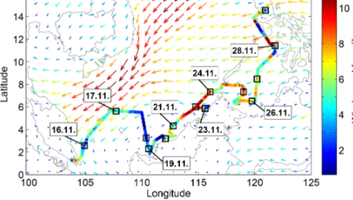
Figure 1.ERA-Interim mean wind field 15–30 November 2011 (ar- rows) and 10 min running mean of wind speed observed on R/V Sonneas the cruise track. The black squares show the ships position at 00:00 UTC each day.

2013; Aschmann and Sinnhuber, 2013). An overview of the data and the methods used in this study is given in Sect. 2.

Section 3 provides results from the meteorological observations along the cruise. Section 4 compares atmospheric VSLS measurements derived on R/V Sonneand R/A Fal- con. The contribution of the oceanic emissions to the MABL and FT air is investigated and discussed in Sect. 5. Finally, a summary of the results is given in Sect. 6.

2 Data and methods

2.1 Ship and aircraft campaigns

The R/VSonnecruise started on 15 November 2011 in Sin- gapore and ended on 29 November 2011 in Manila, Philip- pines (Fig. 1). The ship crossed the southwestern South China Sea towards the northwestern coast of Borneo from 16 to 19 November 2011. From 19 to 23 November 2011 the ship headed northeast along the northern coast of Bor- neo towards the Sulu Sea. Two diurnal stations took place on 18 November 2011 at 2.4^◦N/110.6^◦E and on 22 Novem- ber 2011 at 6.0^◦N/114.8^◦E. Two meetings between ship and aircraft were carried out on 19 and 21 November 2011, where R/A Falcon passed R/V Sonnewithin a distance of about 100 m several times to simultaneously measure the same air masses. On 24 November 2011 the ship entered the Sulu Sea and, after 4 days transect, R/VSonnereached the Philippine coast.

Sixteen measurement flights were carried out with R/A Falconbetween 16 November and 11 December 2011 as part of the SHIVA campaign to investigate halogenated VSLSs from the surface up to 13 km altitude over the South China and Sulu seas. Observations were performed between 1 and 8^◦N, as well as 100 and 122^◦E, from Miri, Borneo (Malaysia), as the aircraft base. A detailed description of the

(3)

VSLS measurements and flight tracks can be found in Sala et al. (2014).

2.2 Meteorological observations during SHIVA 2.2.1 Measurements on board R/VSonne

Meteorological parameters (temperature, air pressure, humidity and wind) were recorded at 20 m height every second.

A 10 min running mean of these data is used for this study.

An optical disdrometer (“ODM-470”) measured the amount and intensity of precipitation during the cruise at 15 m height every minute (see Supplement for further details). To obtain atmospheric profiles of air temperature, relative humidity and wind from the surface to the stratosphere 67 GRAW DFM- 09 and 6 GRAW DFM-97 radiosondes were launched every 6 h at standard UTC times (00:00, 06:00, 12:00, 18:00) from the working deck of R/V Sonneat about 2 m a.s.l. At the 24 h stations, the launch frequency was increased to 2–

3 h to analyse short-term diel variations of the atmospheric boundary layer. The radiosonde data were integrated in near real time into the Global Telecommunication System (GTS) to improve meteorological reanalyses such as ERA-Interim (Dee et al., 2011), which is used as input data for the trajectory calculations (Sect. 5).

2.2.2 Marine atmospheric boundary layer

The MABL is the atmospheric surface layer above the ocean in which trace gas emissions are mixed vertically by convection and turbulence on a short timescale of about an hour (Stull, 1988; Seibert et al., 2000). The upper boundary of the MABL is either indicated by a stable layer, e.g. a temperature inversion, or by a significant reduction in air moisture.

Determination of the MABL height can be achieved by theo- retical approaches, e.g. using critical Bulk Richardson number (Troen and Mahrt, 1986; Vogelezang and Holtslag, 1996;

Sorensen, 1998), or by practical approaches summarised in Seibert et al. (2000). An increase with height of the virtual potential temperature, the temperature an air parcel would acquire if adiabatically brought to standard surface pressure with regard to the humidity of the air parcel, identifies the base of the stable layer, which is typically found between 100 m and 3 km altitude (Stull, 1988). In this study, we use the height of the base of the stable layer increased by half of the stable layer depth as the definition for the MABL height.

The height of the MABL is determined from the atmospheric profiles measured by radiosondes launched on board the ship, as described in detail by Fuhlbrügge et al. (2013).

2.3 VSLS measurements and flux calculation

VSLSs in marine surface air and seawater were sampled synchronously on R/V Sonnealong the cruise track. From these data the oceanic emissions of the compounds during the SHIVA campaign were calculated (Sect. 2.3.3). Addition-

ally, VSLSs were measured in the MABL and the FT by R/A Falcon(Sala et al., 2014; Tegtmeier et al., 2013).

2.3.1 Atmospheric samples

Air samples were taken 3 hourly along the cruise track and 1–2 hourly during the 24 h stations on R/VSonne, resulting in a total of 195 samples during the cruise. The air was pres- surised to 2 atm in pre-cleaned stainless steel canisters with a metal bellows pump. The samples were analysed within 6 months after the cruise at the Rosenstiel School for Marine and Atmospheric Sciences (RSMAS, Miami, Florida) according to Schauffler et al. (1999) with an instrumental precision of∼5 %. Further details of the analysis are described in Montzka et al. (2003) and Fuhlbrügge et al. (2013). On R/AFalcon ambient air was analysed in situ by a GhOST–

MS (gas chromatograph for the observation of stratospheric tracers coupled with a mass spectrometer) by the Goethe University of Frankfurt. Additionally, 700 mL glass flasks were filled with ambient air to a pressure of 2.5 bar with the R/AFalconwhole air sampler (WASP) and analysed within 48 h by a ground-based gas chromatography/mass spectrom- etry (GC/MS) instrument (Agilent 6973) of the University of East Anglia (Worton et al., 2008). During the flights GhOST measurements were conducted approximately every 5 min with a sampling time of 1 min, while WASP samples were taken every 3–15 min with a sampling time of 2 min. Fur- ther details on the instrumental precision and intercalibration on R/AFalcon are given in Sala et al. (2014). Given that the ground-based GC/MS investigated only brominated compounds, CH3I data are not available from WASP. Measure- ments from R/VSonneand R/AFalconwere both calibrated with NOAA standards.

2.3.2 Water samples

VSLS seawater samples were taken 3 hourly from the moon pool of R/V Sonneat a depth of 5 m from a continuously working water pump. Measurements were interrupted between 16 November, 00:00 UTC, to 17 November 2011, 12:00 UTC, due to permission issues in the southwestern South China Sea. The water samples were analysed on board with a purge and trap system, attached to a gas chromatograph with mass spectrometric detection in single-ion mode and a precision of 10 % determined from duplicates. The method is described in detail by Hepach et al. (2014).

2.3.3 Sea–air flux

The sea–air flux (F ) of CHBr₃, CH₂Br₂ and CH₃I is calculated withk_w the concentration gradient and1cthe concentration gradient between the water and atmospheric equi- librium concentrations (Eq. 1). For the determination ofk_w, the wind speed-based parameterization of Nightingale et al. (2000) was used and a Schmidt number (Sc) correction to the carbon dioxide derived transfer coefficientk_CO₂ after

(4)

Quack and Wallace (2003) was applied for the three gases (Eq. 2).

F =kw·1c (1)

k_w=k_CO₂·Sc⁻¹²

600 (2)

Details on calculating the air–sea concentration gradient are further described in Hepach et al. (2014) and references therein.

2.4 Oceanic VSLS contribution to the MABL and FT 2.4.1 Trajectory calculations

The air mass transport from the surface to the FT was calculated with the Lagrangian particle dispersion model FLEX- PART from the Department of Atmospheric and Climate Re- search of the Norwegian Institute for Air Research (Stohl et al., 2005). The model has been extensively evaluated in earlier studies (Stohl et al., 1998; Stohl and Trickl, 1999) and includes parameterisations for turbulence in the atmospheric boundary layer and the FT as well as moist convection (Stohl and Thomson, 1999; Forster et al., 2007). Meteorological input fields are retrieved from the ECMWF (European Centre for Medium-Range Weather Forecasts) assimilation reanalysis product ERA-Interim (Dee et al., 2011) with a horizontal resolution of 1^◦×1^◦and 60 vertical model levels. The ship- based 6-hourly radiosonde measurements were assimilated into the ERA-Interim data (Sect. 2.2.1) and provide air temperature, horizontal and vertical wind, boundary layer height, specific humidity, as well as convective and large-scale precipitation. For the trajectory analysis, 80 release points were defined along the cruise track. Time and position of these release events are synchronised with the water and air samples (Sect. 2.3). At each event, 10 000 trajectories were launched from the ocean surface within a time frame of±30 min and an area of∼400 m²running for 16 days.

2.4.2 VSLS source-loss estimate in the MABL

The timescales of air mass transport derived from FLEX- PART together with the oceanic emissions and chemical losses of the VSLSs are used for a mass balance source-loss estimate over the South China and Sulu seas. For each release event, a box given by the in situ height of the MABL and by the horizontal area of the trajectory releases (∼400 m² centred on the measurement location) is defined. The MABL source-loss estimate is based on the assumption of a constant VSLS mixing ratio (given by the atmospheric measurements), a constant sea–air flux, the chemical loss (CL) rate and a VSLS homogeneous distribution with the box during each release.

The oceanic delivery (OD) is given as the contribution of VSLS sea–air flux (in mol per day) to the total number of

VSLSs in the box (in mol) in percentage per day. The loss of MABL air to the FT caused by vertical transport, denoted here as convective loss (COL), is calculated from the mean residence time of the FLEXPART trajectories in the observed MABL during each release and is given as a negative number in percentage per day. COL equals the loss of VSLSs from the MABL to the FT. The CL, in the form of reaction with OH and photolysis, is estimated in percentage per day (negative quantity) and is based on the tropical MABL lifetime estimates of 15 days for CHBr₃, 94 days for CH₂Br₂ and 4 days for CH₃I (Carpenter et al., 2014).

Relating the delivery of VSLSs from the ocean to the MABL (OD) and the loss of MABL air containing VSLSs to the FT (COL) results in an oceanic delivery ratio (ODR) (Eq. 3):

ODR= OD[% day⁻¹] COL[% day⁻¹]

= sea–air flux contribution[% day⁻¹]

loss of MABL air to the FT[% day⁻¹]. (3) Similarly, the CL in the MABL related to the MABL VSLS loss into the FT (COL) leads to a chemical loss ratio (CLR) (Eq. 4):

CLR= CL[% day⁻¹] COL[% day⁻¹]

= loss through chemistry[% day⁻¹]

loss of MABL air to the FT[% day⁻¹]. (4) The oceanic delivery, chemical loss and loss to the FT must be balanced by advective transport of air masses in and out of the box. We define the change of the VSLSs through advective transport as advective delivery (AD) in percentage per day (Eq. 5). Additionally, we define the ratio of change in VSLSs caused by AD to the loss of VSLSs out of the MABL to the FT as advective delivery ratio (ADR) in Eq. (6):

AD=COL+CL−OD (5)

ADR= AD[% day⁻¹] COL[% day⁻¹]

=1+CLR−ODR. (6) Note that for the VSLSs within the MABL box, COL and CL are loss processes while OD and AD (besides very few exceptions for the latter) are source processes. In order to derive the ratios, we divided CL, OD and AD by COL.

In a final step, we relate the source-loss ratios (ODR, CLR and ADR) to the MABL VSLS volume mixing ratio VMR_MABLin the box (Eqs. 7–9), in order to estimate VSLSs newly supplied from oceanic delivery (VMR_ODR), lost by chemical processes (VMR_CLR) and supplied by advective transport (VMRADR).

(5)

VMR_ODR=ODR·VMR_MABL (7)

VMR_CLR=CLR·VMR_MABL (8)

VMR_ADR=ADR·VMR_MABL (9)

2.4.3 Oceanic and MABL VSLS contribution to the FT We use a simplified approach to calculate the mean contribution of boundary layer air masses observed from various oceanic regions in the South China and Sulu seas on the ship, and the oceanic compounds therein, to the FT. The contribution is determined as a function of time and altitude based on the distribution of the trajectories released at each measurement location along the ship track. According to R/A Falcon observations and our trajectory calculations we assume a well-mixed FT. Observations on R/V Sonne, however, are characterized by large variability and are considered to be representative for the area along the cruise track where the VSLSs were measured in the water and atmosphere. We constrain our calculations to this area and define 80 vertical columns along the cruise track. Each column extends hori- zontally over the area given by the starting points of the trajectories (20 m×20 m centred on the measurement location) and vertically from the sea surface up to the highest point of R/AFalconobservations around 13 km altitude. For each of the 80 columns along the cruise track, 10 000 trajectories were launched and assigned an identical MABL air parcel containing air with the VSLS mixing ratios observed on R/V Sonneduring the time of the trajectory release. The volume of the air parcel is given by the in situ height of the MABL and the horizontal extent of the release box (20 m×20 m) divided by 10 000 trajectories. The transport of the MABL air parcels is specified by the trajectories, assuming that no mixing occurs between the parcels during the transport. Chemi- cal loss of the VSLSs in each air parcel is taken into account through chemical degradation according to their specific tropospheric lifetimes. The VSLS mixing ratios in the FT from the aircraft measurements are considered representative for the entire South China and Sulu seas. Thus we average over the volume and mixing ratios of all trajectories, independent of their exact horizontal location. Due to the decreasing density of air in the atmosphere with height, the volume of the MABL air parcels expands along the trajectories with increasing altitude. The expanding MABL air parcels take up an increasing fraction of air within the FT column, which is taken into account in our calculations using density profiles from our radiosonde measurements.

We calculate the contribution of oceanic compounds to the FT up to 13 km altitude, the upper height of R/AFalconob- servations, within the column above the measurement location. For each layer, the ratio r_MABL of the volume of the MABL air parcels with the VSLS mixing ratio VMR_MABL to the whole air volume of the layer is calculated. The ratio of advected FT air with a mixing ratio VMR_AFT to the

whole air volume of the layer is rAFT respectively, with rMABL+rAFT=1. In our simulation, the FT air with a mixing ratio VMR_FTobserved by R/AFalconat a specific height is composed of the MABL air parcels and of the advected FT air parcels (Eq. 10):

rMABL·VMR_MABL+rAFT·VMR_AFT

=(rMABL+rAFT)·VMRFT. (10) The relative contributionC_MABLof VSLSs observed in the MABL to the VSLSs observed in the FT at heightzand time tis computed in altitude steps of 500 m (Eq. 11):

C_MABL(z, t )[%] =

100·(r_MABL(z, t )·VMR_MABL(CL(t )))/VMR_FT(z).

(11) The oceanic contributionCODR to the VSLSs in the FT is computed after Eq. (12):

CODR(z, t )[%] =

100·(r_MABL(z, t )·VMR_ODR(CL(t )))/VMR_FT(z). (12) The simplified approach also allows deriving mean VSLS mixing ratios accumulated in the FT from both MABL VSLS and oceanic emissions. The FT VSLS mixing ratios are simulated for each of the 80 columns by initiating a new trajectory release event using same meteorological conditions and VSLS MABL observations. The accumulated mean mixing ratio of a compound at a specific heightzis then iterated after Eq. (13):

VMR_FT(z)=

n

X

i=1

(r_MABL(z, t (i))·VMR_MABL(CL(t (i))) +(1−r_MABL(z, t (i)))·VMR_FT(z, t (i−1))

·CL(COL)) . (13)

Here,nis the number of runs for each of the 80 profiles, according to the residence time of the trajectories in the MABL and the total runtime of the trajectories. For example a trajectory residence time of 7 h in the MABL in combination with a total trajectory runtime of 16 days leads ton=(24/7)·16= 54.rMABL gives the volume ratio of MABL air parcels at heightzand timet to the total volume of a specific height layer. VMR_MABL gives the compounds mixing ratio in the air parcels including chemical degradation (CL) since the air was observed in the MABL. Since we use a mean tropospheric lifetime, CL and thus also VMR_MABL(CL) are independent from the heightz. The initial FT background mixing ratios (VMR_FT(z, t (i=0))) are set to 0 ppt for each VSLS, followed byntimes iteration of VMR_FT(i-1). The difference between VMR_FT(i=n−1)and VMR_FT(i=n)during the

(6)

Figure 2.Time series of(a)wind speed (blue) and wind direction (orange) and(b)surface air temperature (SAT, orange) and sea surface temperature (SST, blue) on the left scale, as observed on R/V Sonne. The temperature difference of SAT and SST (1T) is given on the right scale in(b). The1T of 0 K is drawn by a dashed line.

The shaded areas (grey) in the background show the 24 h stations.

The data are averaged by a 10 min running mean.

last two steps of the iteration is less than 1 % for each compound within the 16-day runtime.

The modelled overall mean FT mixing ratio is derived as the mean from the 80 individually calculated FT mixing ratios determined along the cruise. The oceanic contribution to the FT compounds is calculated with VMRODRfrom Eq. (7) inserted as VMRMABLin Eq. (13).

3 Meteorological conditions in the MABL and the FT 3.1 Meteorology along the ship cruise

Moderate to fresh trade winds dominated the South China and Sulu seas during the cruise (Fig. 1a–b), indicated by the overall mean wind direction of northeast (50–60^◦) and a mean wind speed of 5.5±2.9 m s⁻¹. The wind observations reveal two different air mass origins. Between 15 and 19 November 2011 a gentle mean wind speed of 3.7±1.8 m s⁻¹with anorthernwind direction was observed, influenced by a weak low-pressure system (not shown here) over the central South China Sea moving southwest and passing the ship position on 17 November 2011. Dur- ing 20–29 November 2011 the wind direction changed to northeast and the mean wind speed increased to moderate 6.4±3.0 m s⁻¹. A comparison between 6-hourly ERA- Interim wind and a 6-hourly averaged mean of the observed wind on R/V Sonne reveals an underestimation of the wind speed by ERA-Interim along the cruise track by 1.6±1.4 m s⁻¹on average (not shown here). The mean deviation of the wind direction between reanalysis and observation is 2±37^◦. Reanalysis and observed wind speeds cor-

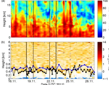
Figure 3. (a) Relative humidity from radiosondes up to 17 km height, the mean cold point tropopause level. The dashed lines and the two numbers above the figure indicate the two 24 h stations.

(b) Virtual potential temperature gradient as indicator for atmospheric stability (red for stable, white for neutral and blue for unstable) with MABL height derived from radiosondes (black curve) and from ERA-Interim (blue curve). Theyaxis is non-linear. The lower 1 km is enlarged to display the stability around the MABL height.

The vertical lines and the two numbers above the figures indicate the two 24 h stations.

relate withR=0.76 and the wind directions withR=0.86, reflecting a good overall agreement between ship observation and ERA-Interim winds. With an observed mean surface air temperature (SAT) of 28.2±0.8^◦C and a mean SST of 29.1±0.5^◦C the SAT is on average 1.0±0.7^◦C below the SST, which benefits convection of surface air (Fig. 2). In- deed, enhanced convective activity and pronounced precipitation events have been observed during the cruise (Fig. S1 in the Supplement). Figure 3a shows the time series of the relative humidity measured by the radiosondes launched on R/VSonne from the surface up to the mean height of the cold point tropopause at 17 km. Elevated humidity is found on average up to about 6 km, which implies a distinct transport of water vapour to the mid-troposphere during the cruise by deep convection or advection of humid air from a nearby convective cell.

3.2 Marine atmospheric boundary layer

Higher SSTs than SATs (Fig. 2) cause unstable atmospheric conditions (negative values of the virtual potential temperature gradient) between the surface and about 50–100 m height (Fig. 3b). Surface air is heated by warmer surface waters and is enriched with humidity both benefiting moist convection. The stability of the atmosphere increases above 420±120 m and indicates the upper limit of the MABL at this altitude range derived from radiosonde data (Fig. 3b).

(7)

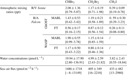
Table 1.Mean±standard deviation and range of atmospheric mixing ratios observed on R/VSonne(195 data points) and R/AFalcon (GhOST–MS with 513 and WASP GC/MS with 202 data points) in the MABL and the FT, water concentrations observed on R/VSonneand the computed sea–air fluxes. MABL and FT mixing ratios on R/AFalconare adopted from Sala et al. (2014) and Tegtmeier et al. (2013).

The R/AFalconMABL height was analysed to be 450 m (Sala et al., 2014).

CHBr₃ CH₂Br₂ CH₃I

Atmospheric mixing R/VSonne 2.08±1.36 1.17±0.19 0.39±0.09

ratios (ppt) [0.79–5.07] [0.71–1.98] [0.19–0.78]

R/A

GhOST

MABL 1.43±0.53 1.19±0.21 0. 59±0.30 Falcon [0.42–3.42] [0.58–1.89] [0.29–3.23]

FT 0.56±0.17 0.87±0.12 0.26±0.11 [0.16–2.15] [0.56–1.54] [0.08–0.80]

WASP

MABL 1.90±0.55 1.15±0.14 / [0.99–3.78] [0.85–1.59]

FT 1.17±0.50 0.88±0.14 / [0.43–3.22] [0.46–1.36]

Water concentrations (pmol L⁻¹) 19.94±17.90 4.99±2.59 3.82±2.43 [2.80–136.91] [2.43–21.82] [0.55–18.84]

Sea–air flux (pmol m⁻²h⁻¹) 1486±1718 405±349 433±482 [−8–13149] [16–2210] [13–2980]

The MABL height given by ERA-Interim along the cruise track is, at 560±130 m, systematically higher (not shown), but still within the upper range of the MABL height derived from the radiosonde measurements. The unstable conditions of the MABL and the increase of the atmospheric stability above the MABL reflect the characteristics of a convective, well-ventilated tropical boundary layer. In contrast to cold oceanic upwelling regions at the coasts with a stable and iso- lated MABL (Fuhlbrügge et al., 2013, 2015), the vertical gradient of the relative humidity measured by the radiosondes (Sect. 3.1) and the height of the MABL do not coincide. This is caused by increased mixing through and above the MABL by turbulence and convection, which leads to the convective, well-ventilated MABL.

4 Atmospheric VSLSs over the South China and Sulu seas

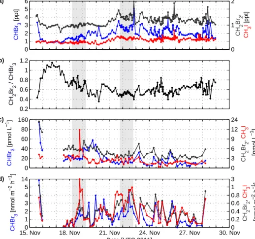
4.1 Atmospheric surface observations on R/VSonne Overall, the three VSLSs show a similar pattern of atmospheric mixing ratios along the cruise track with lower atmospheric surface abundances before 21 November 2011 and higher concentrations afterwards, which can be attributed to a change in air mass origin (Fig. 1). A decrease from 3.4 to 1.2 ppt of CHBr₃ occurs at the beginning of the cruise (Fig. 4a) when the ship left Singapore and the coast of the Malaysian Peninsula. On 16–19 November 2011, when the ship passed the southern South China Sea, lower mixing ratios (±standard deviation 1σ ) of 1.2±0.3 ppt prevail and

also the lowest mixing ratios for CHBr3 during the whole cruise of 0.8 ppt are observed. At the coast of Borneo and the Philippines, the average mixing ratio of CHBr₃increases to 2.3±1.4 ppt. The overall mean CHBr₃mixing ratio during the cruise is 2.1±1.4 ppt (Table 1) and therefore higher than earlier reported CHBr₃ observations of 1.2 ppt in January–

March 1994 (Yokouchi et al., 1997), 1.1 ppt in September 1994 (Quack and Suess, 1999) and 1.5 ppt in June–July 2009 (Mohd Nadzir et al., 2014) further offshore in the South China Sea. The higher atmospheric mixing ratios during the R/VSonnecruise in November 2011 in contrast to the lower mixing ratios in these previous studies may point to stronger local sources, strong seasonal or interannual variations or even to long-term changes. CH2Br2 shows a mean mixing ratio of 1.2±0.2 ppt (Table 1). Yokouchi et al. (1997) observed a lower mean atmospheric mixing ratio of 0.8 ppt and Mohd Nadzir et al. (2014) of 1.0 ppt in the South China Sea.

An increase of the CH₂Br₂mixing ratios from 1.0±0.1 ppt to 1.3±0.2 ppt is observed after 21 November 2011, coinciding with an increase of the CH₃I concentrations from pri- marily 0.3±0.0 ppt to 0.4±0.1 ppt (Fig. 4a). The highest mixing ratio of CH₃I was detected in the southwestern Sulu Sea on 25 November 2011 with 0.8 ppt. The overall mean atmospheric mixing ratio for CH₃I, of 0.4±0.1 ppt (Table 1) is lower than the mean of 0.6 ppt observed by Yokouchi et al. (1997).

The concentration ratio of CH₂Br₂and CHBr₃(Fig. 4b) has been used as an indicator of relative distance to the oceanic source, where a ratio of 0.1 was observed crossing strong coastal source regions (Yokouchi et al., 2005; Carpen-

(8)

CHBr 3 [ppt]

(a)

0 1 2 3 4 5 6

CH 2Br 2, CH 3I [ppt]

0 1 2

CH 2Br 2 / CHBr 3

(b)

0.2 0.4 0.6 0.8 1 1.2

CHBr 3 [pmol L−1]

(c)

0 20 40 60 80 160

CH 2Br 2, CH 3I [pmol L−1]

0 3 6 9 12 24

CHBr 3 [nmol m−2 h−1 ]

(d)

0 1 2 3 4 5 14

CH 2Br 2, CH 3I [nmol m−2 h−1 ]

Date [UTC 2011]

15. Nov 18. Nov 21. Nov 24. Nov 27. Nov 30. Nov0 0.2 0.4 0.6 0.8 1 3

Figure 4.R/VSonnemeasurements of(a)atmospheric mixing ratios of CHBr₃(blue), CH₂Br₂(dark grey) and CH₃I (red);(b)concentration ratio of atmospheric CH₂Br₂and CHBr₃;(c)water concentrations of CH₃I, CHBr₃and CH₂Br₂; and(d)calculated emissions of CHBr₃, CH₂Br₂and CH₃I from atmospheric and water samples. The two shaded areas (light grey) in the background show the 24 h stations.yaxis for(c)and(d)are non-linear.

ter et al., 2003). The 10 times elevated CHBr₃ has a much shorter lifetime, thus degrading more rapidly than CH₂Br₂, which increases the ratio during transport. Overall, the mean concentration ratio of CH₂Br₂and CHBr₃is 0.6±0.2, which suggests that predominantly older air masses are advected over the South China and Sulu seas.

4.2 Oceanic surface concentrations and emissions from R/VSonne

VSLSs in the surface seawater along the cruise track show highly variable distributions (Fig. 4c and Table 1).

Oceanic CHBr₃ surface concentrations range from 2.8 to 136.9 pmol L⁻¹ with a mean of 19.9 pmol L⁻¹ during the cruise, while CH₂Br₂ concentrations range from 2.4 to 21.8 pmol L⁻¹ with a mean of 5.0 pmol L⁻¹. CHBr₃ and CH₂Br₂ have similar distribution patterns in the sampling region with near shore areas showing typically elevated concentrations. CH₃I concentrations range from 0.6 to 18.8 pmol L⁻¹ with a mean of 3.8 pmol L⁻¹ and show a different distribution along the ship track which might be as-

cribed to additional photochemical production of CH₃I in the surface waters (e.g. Manley and Dastoor, 1988; Manley and de la Cuesta, 1997; Richter and Wallace, 2004).

High levels of all VSLSs are found in waters close to the Malaysian Peninsula, especially in the Singapore Strait on 16 November 2011, possibly showing an anthropogenic influence on the VSLS concentrations. VSLS concentrations decrease rapidly when the cruise track leads to open ocean waters. Along the west coast (19–23 November 2011) and northeast coast of Borneo (25 November 2011) bromocarbon concentrations are elevated, and especially CHBr₃ concentrations increase in waters with lower salinities, indicating an influence by river run-off. Elevated CHBr₃concentrations are often found close to coasts with riverine inputs caused by natural sources and industrial and municipal effluents (see Quack and Wallace, 2003; Fuhlbrügge et al., 2013, and references therein).

Oceanic emissions were calculated from synchronised measurements of seawater concentrations and atmospheric mixing ratios, sea surface temperatures and wind speeds, measured on the ship (Sect. 2.3.3). The overall VSLS distri-

(9)

bution along the ship track is opposite for the oceanic and atmospheric measurements (Fig. 4a–d). While the seawater concentrations of VSLSs generally decrease towards the Sulu Sea, the atmospheric mixing ratios increase, leading to a generally lower concentration gradient of the compounds between seawater and air in the Sulu Sea (not shown here).

Coinciding low VSLS atmospheric background concentrations, high SSTs, elevated oceanic VSLS concentrations and high wind speeds, lead to high emissions of VSLSs for the South China and Sulu seas (Fig. 4d) of 1486±1718 pmol m⁻²h⁻¹ for CHBr3, 405±349 pmol m⁻²h⁻¹ for CH2Br2 and 433±482 pmol m⁻²h⁻¹ for CH3I. In particular, CHBr3

fluxes are very high and thus confirm elevated coastal fluxes from previous campaigns in tropical source regions (Quack et al., 2007). They often exceed 2000 pmol m⁻²h⁻¹ in the coastal areas and are sometimes higher than 6000 pmol m⁻²h⁻¹, as in the Singapore Strait on 15 and on 22 November 2011 at the northwestern coast of Borneo, which was also an area of strong convection (Figs. 1, 4b).

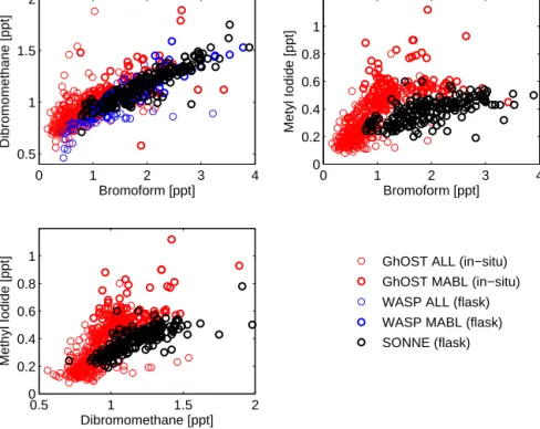
4.3 VSLS intercomparison: R/AFalconand R/VSonne The two profiles of the bromocarbon mixing ratios (Sala et al., 2014) and the profile for CH₃I (Tegtmeier et al., 2013) from the surface to 13 km altitude as observed on R/AFal- con with the GhOST and WASP instruments are shown in Fig. 5. Mean CHBr3mixing ratios are 1.43 ppt (GhOST) and 1.90 ppt (WASP) in the MABL (0–450 m, determined from meteorological aircraft observations similarly as for the radiosondes; Sect. 2.2.2) and 0.56 ppt (GhOST) and 1.17 ppt (WASP) in the FT (0.45–13 km; Table 1). The GhOST mixing ratios in the MABL are lower than those observed on R/V Sonne(2.08 ppt). A very good agreement of the measurements is given for the longer lived CH₂Br₂with 1.17 ppt (R/VSonne), 1.19 ppt (GhOST) and 1.15 ppt (WASP). CH₃I mixing ratios measured by GhOST are 0.59±0.30 ppt within the MABL of 450 m height, which is about 0.2 ppt higher than the values from R/V Sonne. Above the MABL, the average mixing ratio of CH₃I decreases to 0.26±0.11 ppt (Fig. 5).

CHBr3 and CH2Br2 concentrations in the MABL correlate with R=0.83 for all instruments (Fig. 6). CHBr3and CH3I concentrations correlate withR=0.55 and CH2Br2

and CH3I withR=0.66; all correlations are significant at 99 %. Even higher correlations are found if only measurements on R/V Sonneare taken into account withR=0.92 for CHBr₃and CH₂Br₂,R=0.64 for CHBr₃and CH₃I and R=0.77 for CH₂Br₂and CH₃I.

Comparisons of R/AFalconand R/VSonnedata are ob- tained from their meetings on 19 and 21 November 2011 (Table 2), when aircraft and ship passed each other within 100 m distance several times, measuring the same air masses.

During both meetings, deviations between the GhOST and WASP instruments on the aircraft are larger for the bromo-

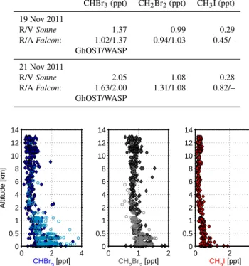
Table 2.Mean atmospheric mixing ratios of CHBr₃, CH₂Br₂and CH₃I observed on R/VSonneand R/AFalconduring two case studies on 19 November 2011 at 3.2^◦N and 112.5^◦E and on 21 Novem- ber 2011 at 4.6^◦N and 113.0^◦E. During the two meetings two (one) measurements have been taken by R/VSonne, 20 (5) measurements on R/AFalconby GhOST and 17 (21) by WASP.

CHBr₃(ppt) CH₂Br₂(ppt) CH₃I (ppt) 19 Nov 2011

R/VSonne 1.37 0.99 0.29

R/AFalcon: 1.02/1.37 0.94/1.03 0.45/–

GhOST/WASP 21 Nov 2011

R/VSonne 2.05 1.08 0.28

R/AFalcon: 1.63/2.00 1.31/1.08 0.82/–

GhOST/WASP

CHBr₃ [ppt]

Altitude [km]

0 2 4

0 0.5 1 2 4 6 8 10 12 14

CH₂Br₂ [ppt]

0 1 2

0 0.5 1 2 4 6 8 10 12 14

CH₃I [ppt]

0 2

0 0.5 1 2 4 6 8 10 12 14

Figure 5.Vertical distribution CHBr₃(blue), CH₂Br₂(grey) and CH₃I (red) mixing ratios measured in situ by GhOST (diamonds) and with flasks by WASP (circles) on R/AFalcon. CH₃I was only measured in situ by GhOST. The lower 2 km are non-linear dis- played.

carbons than the deviation between the WASP and the ship measurements. According to Sala et al. (2014) the agreement between the GhOST and WASP instruments is within the ex- pected uncertainty range of both instruments, which is then assumed to be also valid for the ship measurements (this study). The good agreement between WASP and ship data might be caused by the same sampling and analysis method, both using stainless steel canisters and subsequent analysis with GC/MS, while GhOST measures in situ with a different resolution. Since GhOST and WASP measurements together cover a larger spatial area and higher temporal resolution, a mean of both measurements is used in the following for computations in the free troposphere. For CH3I significantly higher mixing ratios were measured with GhOST during the meetings between ship and aircraft (Table 2). Whether this offset is systematic for the different methods needs further investigation.

(10)

0 1 2 3 4 0.5

1 1.5 2

Bromoform [ppt]

Dibromomethane [ppt]

0 1 2 3 4

0 0.2 0.4 0.6 0.8 1

Bromoform [ppt]

Metyl Iodide [ppt]

0.5 1 1.5 2

0 0.2 0.4 0.6 0.8 1

Dibromomethane [ppt]

Methyl Iodide [ppt]

GhOST ALL (in−situ) GhOST MABL (in−situ) WASP ALL (flask) WASP MABL (flask) SONNE (flask)

Figure 6.Correlation of bromoform and CH₂Br₂(upper left), bromoform and CH₃I (upper right), and CH₂Br₂and CH₃I (lower left) from GhOST and WASP for all heights (ALL) and only within the MABL (MABL) and from R/VSonne.

Date [UTC 2011]

Height [km]

30

30 30

30

30 30

50 50

50

50 50

50 50 50

50 50

50 50 7070

70

70 70

70

70 70

70 90 90

16.11. 19.11. 22.11. 25.11. 28.11.

0 2 4 6 8 10 12

Days after release

0 2 4 6 8 10

Figure 7.Forward trajectory runs along the cruise track with FLEX- PART using ERA-Interim data. The black contour lines show the mean amount of trajectories (in %) reaching a given height within the specific time (colour shading). The white line indicates the radiosonde MABL height.

5 Air mass and VSLS transport from the surface to the free troposphere

5.1 Timescales and intensity of vertical transport Forward trajectories computed with FLEXPART starting at sea level along the cruise track yield an average MABL residence time of 7.8±3.5 h before the trajectories enter the FT (Fig. 7), reflecting a relatively fast exchange due to the convective well-ventilated MABL (Fig. 3). The trajectories generally show a strong contribution of surface air masses

to the FT, despite some exceptions during 18–22 Novem- ber 2011 (Fig. 7). Most intense and rapid transport of MABL air masses up to 13 km height occurs on 17 and 23 Novem- ber 2011.

5.2 Contribution of oceanic emissions to VSLSs in the MABL

From the sea–air fluxes (Sect. 4.2) and the residence times of the surface trajectories in the MABL (Sect. 5.1), the OD and the COL were computed (Table 3) using the method described in Sect. 2.4.2.

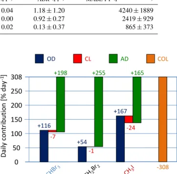
Based on the OD and the COL, the ODR is calculated in order to characterise the relative contribution of the local oceanic emissions compared to the loss of MABL air into the FT (Table 3, Fig. 8). The average ODR during the cruise is 0.45±0.55 for CHBr3, which means that the loss from the MABL to the FT is balanced to 45 % by oceanic emissions along the cruise track. The ODR for CH2Br2 is 0.20±0.21 and for CH3I 0.74±1.05 respectively, suggesting that the major amount of CH₃I originates from nearby sources. Similarly to the ODR the CL is related to the COL to derive the CLR for the VSLSs, which is 0.03±0.01 for CHBr₃, 0.01±0.00 for CH₂Br₂and 0.09±0.04 for CH₃I. When compared to the other source and loss processes, the chemical loss appears negligible for all three gases. The ratio of the ADR is 0.58±0.55 for CHBr₃, 0.80±0.21 for CH₂Br₂ and 0.35±1.02, implying that most of the observed CH₂Br₂ (80 %) in the MABL is

(11)

Table 3.Mean±standard deviation of oceanic delivery (OD), convective loss (COL), chemical loss (CL), advective delivery (AD), oceanic delivery ratio (ODR), chemical loss ratio (CLR) and advective delivery ratio (ADR) for CHBr₃, CH₂Br₂and CH₃I.

OD (% day⁻¹) COL (% day⁻¹) CL (% day⁻¹) AD (% day⁻¹) ODR CLR ADR CHBr₃ 116.4±163.6 307.6±124.3 7.1 198.2±199.7 0.45±0.55 0.03±0.01 0.58±0.55 CH₂Br₂ 54.2±66.7 307.6±124.3 1.2 254.6±131.9 0.20±0.21 0.00±0.00 0.80±0.21 CH₃I 166.5±185.8 307.6±124.3 24.0 165.2±242.3 0.74±1.05 0.09±0.04 0.35±1.02

Table 4.Mean±standard deviation of observed mixing ratios in the MABL on R/VSonne(VMR_MABL)vs. the amount of VMR originating from oceanic emissions (VMR_ODR), chemically degraded according to the specific lifetime (VMR_CLR), originating from advection (VMR_ADR)and the flux from the MABL into the FT (flux_MABL-FT)for CHBr₃, CH₂Br₂and CH₃I.

VMR_MABL(ppt) VMR_ODR(ppt) VMR_CLR(ppt) VMR_ADR(ppt) Flux_MABL-FT(pmol m⁻²h¹)

CHBr₃ 2.08±1.36 0.89±1.12 −0.06±0.04 1.18±1.20 4240±1889

CH₂Br₂ 1.17±0.19 0.25±0.26 −0.01±0.00 0.92±0.27 2419±929

CH₃I 0.39±0.09 0.28±0.40 −0.04±0.02 0.13±0.37 865±373

Table 5. Correlation coefficients between wind speed and VSLS MABL mixing ratios (VMR_MABL), the oceanic delivery (OD), the convective loss (COL) to the FT, the advective delivery (AD), computed as the residual of OD, and the mixing ratios originating from the OD (VMR_ODR)and from the AD (VMR_ADR)of each compound. Bold numbers are significant at the 95 % level (pvalue).

Wind speed CHBr₃ CH₂Br₂ CH₃I

VMR_MABL 0.55 0.57 0.56

OD 0.31 0.48 0.52

COL −0.33

AD −0.46 0.56 −0.57

VMR_ODR 0.52 0.72 0.62

VMR_ADR −0.17 −0.31 −0.49

advected from other source regions. Applying the ODR to the observed mixing ratios in the MABL gives an estimate of the VSLSs originating from the local oceanic emissions (VMR_ODR, Table 4). The local ocean emits a concentration that equates to 0.89±1.12 ppt CHBr₃, 0.25±0.26 ppt CH₂Br₂ and 0.28±0.40 ppt CH₃I in the MABL. The average transport from the MABL to the FT (fluxMABL-FT), computed from the MABL concentrations and the trajectory residence time in the MABL, is 4240±1889 pmol m⁻²h⁻¹ for CHBr3, 2419±929 pmol m⁻²h⁻¹ for CH2Br2 and 865±373 pmol m⁻²h⁻¹ for CH3I. Calculations with the ERA-Interim MABL height, which is on average 140 m higher than the one derived from the radiosondes, leads to similar estimates (Table S1).

Since the wind is a driving factor for oceanic emissions and advection of VSLSs, changes in wind speed are assumed to affect atmospheric VSLS mixing ratios in the MABL during this cruise. Significant correlations are found between wind speed and the observed mixing ratios of all three VSLSs in the MABL with correlation coefficients

308

200 150 100 50

-1Daily contribution [% day] 0

OD CL AD

250

+116 -7

+198

+54 -1

+255

+167 -24

+165

-308 COL

Figure 8. Average budgets of the oceanic delivery (OD, blue), chemical loss (CL, red), advective delivery (AD, green) and convective loss (COL, orange) of CHBr₃, CH₂Br₂and CH₃I in the marine atmospheric boundary layer (MABL).

of R=0.55 (CHBr3), R=0.57 (CH2Br2) and R=0.56 (CH3I) respectively (Table 5). Mixing ratios that originate from oceanic emissions (VMRODR)correlate significantly to the wind speed withR=0.52,R=0.72 andR=0.62 respectively. In contrast, VMR_ADR, which is calculated as the residual from VMR_ODR, is negatively correlated to the wind speed withR= −0.21,R= −0.32 andR= −0.53. The correlations reveal that the contribution of oceanic emissions to MABL VSLSs increase for higher wind speeds, while the advective contribution decreases.

(12)

1

1 1

2

2 3

3 3 3

5

10 10

Height [km]

Bromoform (a)

0 5 10 15 0.5

2 4 6 8 10 12

0.1 0.2 0.3 0.5 0.7 1 2 3 5 7 10 20 30 50

1

1 1

2

2 3

3 3 3

5

10 10 Dibromomethane (b)

0 5 10 15 0.5

2 4 6 8 10 12

0.1 0.2 0.3 0.5 0.7 1 2 3 5 7 10 20 30 50

1

1 1

2

2 3

3 3 3

5

10 10 Methyl iodide (c)

0 5 10 15 0.5

2 4 6 8 10 12

MABL contribution [%]

0.1 0.2 0.3 0.5 0.7 1 2 3 5 7 10 20 30 50

1

1 1

2

2 3

3 3 3

5

10 10

Days after release

Height [km]

(d)

0 5 10 15 0.5

2 4 6 8 10 12

0.1 0.2 0.3 0.5 0.7 1 2 3 5 7 10 20 30 50

1

1 1

2

2 3

3 3 3

5

10 10

Days after release (e)

0 5 10 15 0.5

2 4 6 8 10 12

0.1 0.2 0.3 0.5 0.7 1 2 3 5 7 10 20 30 50

1

1 1

2

2 3

3 3 3

5

10 10

Days after release (f)

0 5 10 15 0.5

2 4 6 8 10 12

Oceanic contribution [%]

0.1 0.2 0.3 0.5 0.7 1 2 3 5 7 10 20 30 50

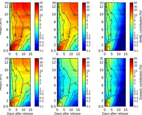
Figure 9.Mean MABL air contribution(a–c)and oceanic contribution(d–f)to observed FT mixing ratios observed by R/AFalconfor three VSLSs. The black contour lines show the mean portion of MABL air masses in the FT (%), the colours show the oceanic contribution to the observed compounds in the FT at specific height and day after release (%) including chemical degradation and the vertical density driven extension of MABL air masses. The scale of the coloured contour is logarithmic.

5.3 Oceanic contribution to the FT

5.3.1 Identification of VSLS MABL air in the FT With a simplified approach (method description in Sect. 2.4.3) we are able to estimate the contribution of MABL air and regional marine sources observed on R/V Sonne to the FT. Individual MABL air masses during the cruise show a strong contribution to the FT air up to 10 % after 10 days (Fig. 9a–f). The MABL air is rapidly transported into high altitudes before it is dispersed in the FT column.

The average contribution of VSLS concentrations in the MABL air to the FT concentrations (CMABL)is generally highest for CHBr3, with 10–15 % between 4 and 10 km and up to 25 % above 10 km height 3–10 days after release in the MABL (coloured contours in Fig. 9a), followed by CH2Br2

(5–10 % below 10 km and up to 16 % above 10 km height;

Fig. 9b). The lowest contribution is found for the short- lived CH₃I with up to 4 % within 3 days (Fig. 9c). In gen- eral the contribution below 5 km height decreases after about 10 days, when most of the MABL air is transported into higher altitudes. For CH₃I, the chemical degradation, according to its short tropospheric lifetime of 3.5 days, leads to a rapid decrease of the contribution already 3 days after release.

To identify the contribution of the oceanic emissions to the FT VSLSs during the cruise, the VMRODR of each compound is used as the initial mixing ratio in the MABL air mass. For CHBr₃and CH₂Br₂ the local emissions contribute only up to 11 and 4 % to the FT concentrations (C_ODR; Fig. 9d–e) compared to the 25 %, respectively 16 %, ofC_MABL. In contrast, the contribution of the local oceanic emissions of CH₃I (Fig. 9f) is almost similar to the contribution of the observed MABL concentrations (Fig. 9c).

5.3.2 Accumulated VSLSs in the free troposphere By simulating a steady transport of MABL air masses into the FT, mean accumulated VSLS mixing ratios in the FT along and during the cruise were computed (Fig. 10) as described in Sect. 2.4.3. The simulated FT mixing ratios of CHBr3and CH2Br2from the observed MABL (VMRMABL) decrease on average from 2.1 and 1.2 ppt at the surface to 0.6 and 0.8 ppt at 3 km height. The simulated CHBr₃ mixing ratios are constant up to 8 km height followed by an increase up to 0.9 ppt at 13 km height. Simulated CH₂Br₂ mixing ratios increase between 3 and 11.5 km height up to 1.1 ppt and remain constant above 11.5 km height. Simulated CH₃I shows a decrease from 0.4 ppt at the surface to 0.08 ppt at 3 km. Above this altitude, the simulated mixing ratios of CH₃I are almost constant before they slowly increase above 9 km height to 0.10 ppt.

(13)

Height [km]

[ppt]

Bromoform

0 0.5 1 1.5 2 2.5 0

2 4 6 8 10 12

[ppt]

Dibromomethane

0 0.5 1 1.5 0

2 4 6 8 10 12

[ppt]

Methyl iodide

0 0.2 0.4 0.6 0

2 4 6 8 10 12

Obs.

Obs.*

sMABL sOcean

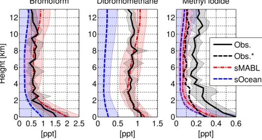
Figure 10.Mean FT mixing ratios (solid lines) and 1 standard deviation (shaded areas) from in situ and flask observations on R/AFalcon (Obs., black) vs. simulated mean FT mixing ratios from MABL air (sMABL, red) and oceanic emissions (sOcean, blue) observed by R/V Sonne. R/AFalconin situ observations have been adjusted for CH₃I (Obs.^∗, dashed black) according to measurement deviations during the meetings of R/VSonneand R/AFalcon(Table 2; Sect. 4.3).

To estimate the accumulated FT mixing ratios solely from oceanic emissions, the VMR_ODRis used as the initial MABL mixing ratio (Fig. 10). The simulated FT mixing ratios using either VMR_MABLor VMR_ODRas input reveal a similar vertical pattern, since both simulations are based on the same meteorology and trajectories. While FT mixing ratios based on VMRMABLand VMRODRare similar for CH3I and differ by about 0.03 ppt (due to the large oceanic contribution to the MABL mixing ratios), FT mixing ratios from VMRODRare on average∼0.4 ppt lower for CHBr3and∼0.8 ppt CH2Br2

than from VMR_MABL. Comparing the simulated VMR_MABL FT mixing ratios with the observed FT mixing ratios from R/AFalconreveals generally stronger vertical variations for the observations in contrast to the simulations. Still, CHBr₃ observations are well reflected in the VMR_MABLsimulation between 2 and 11 km altitude. Also the simulated CH₂Br₂ in the FT based on VMR_MABL reflects the observations of R/A Falcon very well from the surface up to 9 km height.

The CH₃I simulations show a distinct underestimation of the observed FT mixing ratios. Adjusting the R/AFalconvalues by the identified offset to R/VSonne(Sect. 4.3 and Table 2) reveals a better agreement between observed and simulated FT mixing ratios (Fig. 10).

5.3.3 Discussion

Oceanic emissions of CHBr₃from the South China and Sulu seas contribute on average 45 % to the simulated FT mixing ratios (Fig. 10). Simulated FT mixing ratios from MABL observations and observed FT mixing ratios agree quite well up to 11 km height. Above this altitude the simulated FT mixing ratios, in contrast to the observations increase, which is caused by an overestimation of the convective activity in

our method. However, despite using this simple approach we are able to simulate mean FT mixing ratios up to 11 km height above the South China and Sulu seas in good agreement with observations. Thus, we assume that the observed MABL mixing ratios of CHBr₃and CH₂Br₂are representative for the South China and Sulu seas.

On average, 45 and 20 % of CHBr3 and CH2Br2 abundances in the MABL, observed on the ship, originate from local oceanic emissions along the ship track. Thus, advection from stronger source regions, possibly along the coast (for CHBr₃)and from the West Pacific (CH₂Br₂), are neces- sary to explain the observed MABL mixing ratios.

In contrast to CHBr₃and CH₂Br₂, the simulated mixing ratios of CH₃I in the FT are strongly underestimated regard- less of whether observed MABL mixing ratios or oceanic emissions are used. The offset between the simulated and observed FT CH₃I could be caused by additional strong sources of CH₃I in the South China and Sulu seas. Furthermore, mod- elling or measurement uncertainties may add to this offset.

The simulations use constant atmospheric lifetimes for each compound and neglect lifetime variations with altitude which could impact the simulated abundances. However, the altitude variations of the CH3I lifetime in the MABL and FT are around 0.5 days (Carpenter et al., 2014) and thus impacts on the simulated abundances are quite small. Therefore, it seems unlikely that the lifetime estimate causes a large underestimation of the FT CH₃I. Additional uncertainties may arise from cloud-induced effects on photolysis rates (Tie et al., 2003) and OH levels (e.g. Tie et al., 2003; Rex et al., 2014) impacting the VSLS lifetimes. Deficiencies in the meteorological input fields and the FLEXPART model, in particular in the boundary layer and in the convection parame-